Machine Learning Interatomic Potentials with Keras API
Abstract
A neural network is used to train, predict, and evaluate a model to calculate the energies of 3-dimensional systems composed of Ti and O atoms. Python classes are implemented to quantify atomic interactions through symmetry functions, and to specify prediction algorithms. The hyperparameters of the model are optimised by minimising validation RMSE, which then produced a model that is accurate to within 100 eV. The model could be improved by proper testing of symmetry function calculations and addressing properties of features and targets.
I Introduction
Density functional theory (DFT) is a widely-used method for calculating properties of atomic structures, which typically contain a significant number of atoms, such as the arrangement of crystals and sizable molecules [1]. While accurately predicting the structural behaviours, it has been observed that DFT is computationally expensive [1], and effort has been made in the past years into optimising algorithms for faster and more accurate computation [2].
Some studies have proposed that the use of machine learning methods can improve performance when calculating inter-atomic potentials [3, 4]. Behler and Parinello (2007), suggested the use of a neural-network (NN) model that predicts the energy of a set of atoms in bulk silicon. It was shown to be more accurate and has faster predicting times than DFT. In 2015, Artrith and Urban implemented the Behler-Parinello neural-network (BPNN) architecture in Fortran, predicting the total energies in TiO2 crystals. In this paper, we implement and evaluate a similar, but smaller, NN through the Keras API [5] in Python and using the Atomic Energy network (aenet) TiO2 dataset [6].
II Theory
The BPNN utilises a set of functions called the radial (RSF, denoted as ) and angular symmetry functions (ASF, ) to detail two and three-body atomic interactions respectively. For a system with atoms, the radial symmetry function for an atom with coordinates is written as
| (1) |
and the angular symmetry function is
| (2) | ||||
The arguments are free parameters, can be different for (1) and (2), and . The parameters vary depending on the chemical composition, and therefore bonding, of the crystals. Here, the cutoff function is introduced, where it describes how physically significant the atomic interaction is, written as
with as the cutoff parameter.
These sets of SFs are the inputs for the NN, which is composed of identical subnets. For each atom in the system, its associated ASF and RSF is “fed-forward” to the layers in the network to obtain an associated energy , the contribution of that atom to the entire system. Then the total energy is the linear sum of the contributions, i.e.:

It is also important to take account of different possibilities of chemical bonds [6] like Ti–O, Ti–Ti, and O–O, which means that the parameters in the SFs may vary. To mitigate, different parameter values and combinations are added to the input, where instead of just a pair of ASF and RSF, it is a set of each; that is, the NN optimises which of the symmetries contribute more to the total energy. A schematic diagram for a subnet can be seen in Figure 1.
III Methods
III.1 Data Preprocessing
Before training and evaluating the model, the data undergoes extensive data processing. The energies (our targets) are extracted, and the SFs (the feature space) are computed. The aenet dataset contains 7815 *.xsf files, with each containing the total energy in eV, a set of coordinates for the unit cell of the crystal, and its primitive vectors, which dictates the vector basis of periodicity (i.e. an atom system with the origin has translational symmetry when transforming into , with ).
The energies are extracted into a *.csv file through a Python script called xsf_clean.py. Then, a Python class SymmetryCalculator is used to calculate the SF of all atoms in each system. Specifically, the class reads the dataset and for each structure, the positions are duplicated to emulate a periodic structure using the primitive vectors and positions, then with the parameters, the s and s are calculated. The full parameter set is outlined in Tables I and II of Ref. [6], however, only 14 out of the full 70+ parameters are used due to hardware and computing time limitations. The SFs are then written to a file with the name symXXXX.csv, with XXXX being a four-digit index of the structure.
III.2 Model Implementation
As for the model itself (BPNN), it subclasses from the keras.Model class. The subnet takes in a list of keras.layers classes where it is instantiated as a Sequential object. When calling the object for fitting or evaluating, the second axis of the feature space with size (batch_size, n_atoms, n_symmetries) is split, and passed through the model one row at the time, where it produces an energy contribution. After iterating through all the atoms in the structure and following section II, we now then have a collection of contributions, where its sum is taken. All project files can be found in Ref. [7]
III.3 Data Analysis
The model is compiled using the mean absolute error (MAE) as loss and the root mean squared error (RMSE) as the metric to evaluate model performance. To optimise the weights and biases, we use the adaptive moment estimation (ADAM) optimisation algorithm as it is adaptive and efficient [8]. The GridSearch class from KerasTuner’s hyperparameter (HP) tuning library is used to find the best NN. The specific values used for each HP is shown in Table 1.
| HP | values |
|---|---|
| number of layers | 4, 5, 6 |
| number of nodes per layer | 16, 32, 64 |
| learning rate | , , |
| dropout | True, False |
IV Results
Out of 7815 structures, only 265 symmetry files are generated due to long computing times.
| HP | values |
|---|---|
| number of layers | 5 |
| number of nodes per layer | 64 |
| learning rate | |
| dropout | False |
Tuning the model by minimising validation RMSE, we find the parameters in Table 2. The best HPs obtained have the RMSE eV.
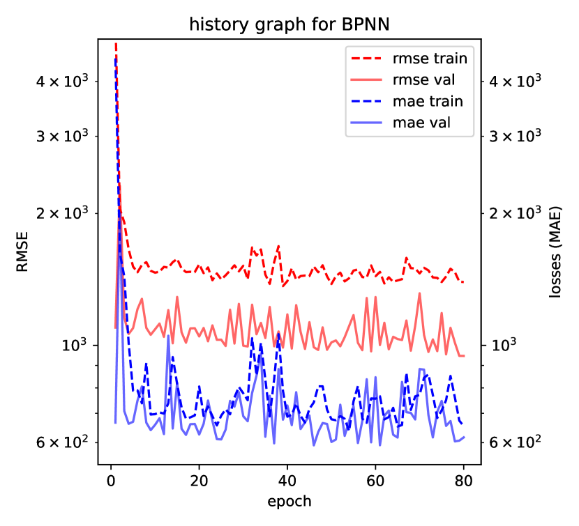
Fitting the best model with batch size 20 and 80 epochs, it is seen that the model converges by epoch 10 (Figure 2), which appears to have a validation loss of 600 eV MAE at higher epochs.
Its residuals have a sample mean of eV and a standard error of eV. is also the RMSE of the testing data. Thus, it is more motivational to rewrite is as RMSE eV
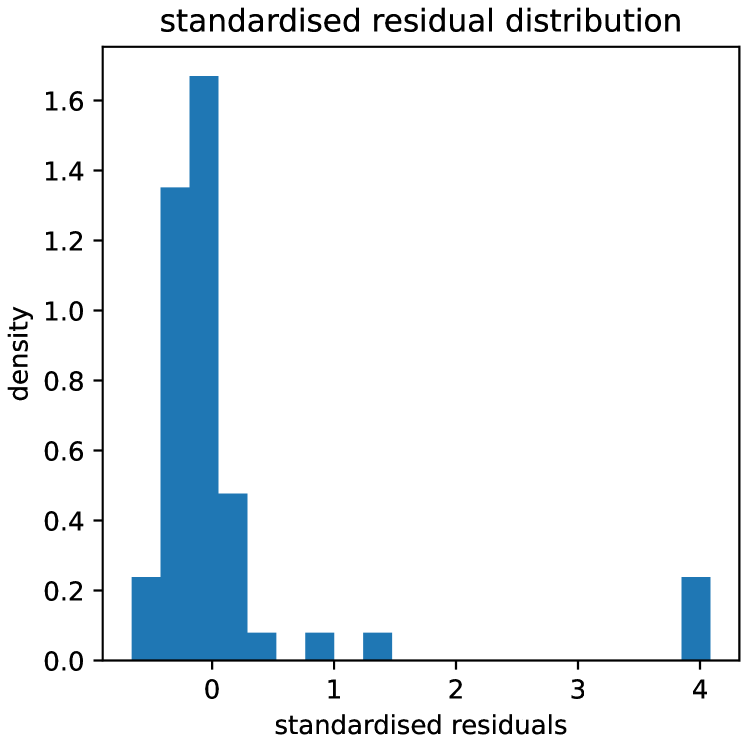
Standardising and normalising the distribution produces the residual plot figure 3. The proportion of the predictions outside of the true target values (outlier fraction) is equal to .
V Discussion & Summary
Comparing RMSE and the magnitude of values for the targets, it can be said that the energy calculations are accurate up to a hundred eV. The inaccuracy could be caused by several issues in the symmetry calculation or parameter fitting. Firstly, the amount of data processed is only approximately of the total dataset, containing only 25 atoms per structure, whereas the dataset contains structures with 6, 25, 47, and 95 atoms. The BPNN predicting other systems with differing unit cell size would yield great errors as uncertainties would come from extrapolation.
Another is the inaccuracy of the ASF calculation. Due to time constraints, SymmetryCalculator lacks proper testing so there is a possibility that the calculated RSFs and ASFs are incorrect. In the future, more optimisation should be made to the implementation such as introducing multiprocessing, rewriting the code in a compiled, lower-level language like C/C++, or integrating well-tested libraries to the implementation.
Another concerns the number of parameters used in the symmetry calculation. The parameters for this implementation are reduced, and this reduction makes it seem that only one chemical species is present, which will also introduce errors in prediction.
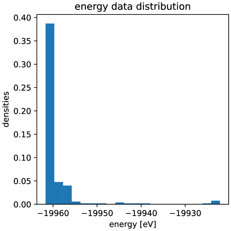
More importantly, the data imbalance that the set has affects the quality of the fitting. Standardising and normalising the distribution produces the residual plot figure 3. Inspecting the energy distribution of the dataset (see Figure 4), we see a significant amount of values that lie just under eV. This will introduce unwanted bias to the data towards its most common target value.
In summary, the BPNN is implemented in Python through the Keras API. Using radial and angular interactions of atoms, crystalline structures composed of Ti and O atoms are regressed to predict the energies of their corresponding unit cells. Tuning the hyperparameters gives predictions with accuracy up to 100 eV, which can be improved by the processing more structures and accounting for the imbalanced distribution of the energy data.
References
- Bretonnet [2017] J.-L. Bretonnet, Basics of the density functional theory, AIMS Materials Science 4, 1372 (2017).
- Hu and Chen [2021] W. Hu and M. Chen, Editorial: Advances in density functional theory and beyond for computational chemistry, Frontiers in Chemistry 9, 10.3389/fchem.2021.705762 (2021).
- Behler and Parrinello [2007] J. Behler and M. Parrinello, Generalized neural-network representation of high-dimensional potential-energy surfaces, Phys. Rev. Lett. 98, 146401 (2007).
- Karniadakis et al. [2021] G. E. Karniadakis, I. G. Kevrekidis, L. Lu, P. Perdikaris, S. Wang, and L. Yang, Physics-informed machine learning, Nature Reviews Physics 3, 422 (2021).
- O’Malley et al. [2019] T. O’Malley, E. Bursztein, J. Long, F. Chollet, H. Jin, L. Invernizzi, et al., Kerastuner, https://github.com/keras-team/keras-tuner (2019).
- Artrith and Urban [2016] N. Artrith and A. Urban, An implementation of artificial neural-network potentials for atomistic materials simulations: Performance for tio2, Computational Materials Science 114, 135 (2016).
- [7] J. P. Rili, Machine Learning Interatomic Potentials with Keras API.
- Kingma and Ba [2017] D. P. Kingma and J. Ba, Adam: A method for stochastic optimization (2017), arXiv:1412.6980 [cs.LG] .