Sequential monitoring for explosive volatility regimes

Abstract.

In this paper, we develop two families of sequential monitoring procedure to (timely) detect changes in a GARCH(1,1) model. Whilst our methodologies can be applied for the general analysis of changepoints in GARCH(1,1) sequences, they are in particular designed to detect changes from stationarity to explosivity or vice versa, thus allowing to check for “volatility bubbles”. Our statistics can be applied irrespective of whether the historical sample is stationary or not, and indeed without prior knowledge of the regime of the observations before and after the break. In particular, we construct our detectors as the CUSUM process of the quasi-Fisher scores of the log likelihood function. In order to ensure timely detection, we then construct our boundary function (exceeding which would indicate a break) by including a weighting sequence which is designed to shorten the detection delay in the presence of a changepoint. We consider two types of weights: a lighter set of weights, which ensures timely detection in the presence of changes occurring “early, but not too early” after the end of the historical sample; and a heavier set of weights, called “Rényi weights”  which is designed to ensure timely detection in the presence of changepoints occurring very early in the monitoring horizon. In both cases, we derive the limiting distribution of the detection delays, indicating the expected delay for each set of weights. Our theoretical results are validated via a comprehensive set of simulations, and an empirical application to daily returns of individual stocks.

1. Introduction

In recent years, developing tools for the (ex-ante or ex-post) detection of the onset or the collapse of a bubble in financial markets has been one of the most active research areas in financial econometrics; we refer the reader, in particular, to the seminal articles on ex-post detection by Phillips et al. (2011), and Phillips et al. (2015a), and also to Skrobotov (2023) for a review. As far as ex-ante detection - that is, finding the onset or collapse of a bubble in real time, as new data come in - is concerned, this important issue has also been studied in numerous recent contributions; although a comprehensive literature review goes beyond the scope of this paper, we refer to the articles by Homm and Breitung (2012), Phillips et al. (2015b), and Whitehouse et al. (2023), inter alia; in particular, the paper by Whitehouse et al. (2023) also contains a comprehensive literature review of in-sample and online bubble detection methods. A common trait to the vast majority of the existing literature is its reliance on a linear specification, usually an AutoRegressive (AR) model, to capture regime changes in the dynamics of log prices. Whilst such a modelling choice can be justified from the theoretical point of view (see e.g. Phillips and Yu, 2011), and whilst its analytical tractability offers obvious advantages from a mathematical standpoint (see e.g. Phillips and Magdalinos, 2007, and Aue and Horváth, 2007), a major issue is that using an AR model is fraught with difficulties when monitoring for changes from an explosive towards a stationary regime. Several promising solutions have been proposed such as the reverse regression approach by Phillips and Shi (2018). Horváth and Trapani (2023) propose a different model, based on a Random Coefficient Autoregressive (RCA) specification, where inference is always standard normal irrespective of stationarity or the lack thereof (Aue and Horváth, 2011), and develop a family of sequential monitoring procedures based on the weighted CUSUM process, to check whether the deterministic part of the autoregressive root changes over time. Such a testing set-up also encompasses both the case of a switch from a stationary to an explosive regime (thus indicating the start of a bubble phenomenon), and a change from an explosive to a stationary regime (thus signalling the collapse of a bubble).

The theory developed in Horváth and Trapani (2023) paves the way to a more general research question, namely developing sequential monitoring techniques which are robust to both the initial regime (i.e., which can be employed irrespective of whether the observations in the training/historical sample are stationary or explosive), and to the type of change which occurs after a changepoint (i.e., which can detect changes from stationarity to another stationary regime, or to a explosive regime; or from an explosive regime to another explosive regime or a stationary one). From a technical viewpoint, this question is nontrivial for at least three reasons. First, proposing a changepoint detection methodology whose asymptotics is the same irrespective of stationarity or explosivity is not easy per se, because the partial sum processes which constitute the building blocks of e.g. CUSUM-based statistics require completely different approximations depending on whether the observations are stationary or not. Second, in order to ensure timely changepoint detection, weighted versions of the CUSUM process need to be considered, with different sets of weights ensuring optimal detection delays for different changepoint locations within the monitoring horizon. Third, on account of the previous point, it is important to offer, to the applied user, a battery of results on the limiting distribution of the detection delays, so as to gauge the expected detection delay depending on the location of the changepoint and the weighing scheme employed.

Motivated by the questions above, in this paper we investigate, with an emphasis on completeness, the issue of sequential detection for regime changes in a GARCH(1,1) sequence

(1.1) $$y_{i}=\sigma_{i}\epsilon_{i}\quad\;\;\mbox{and}\quad\;\;\sigma_{i}^{2}=\omega+\alpha y_{i-1}^{2}+\beta\sigma_{i-1}^{2},\;\;\;1\leq i<\infty.$$

In particular, we develop two families of detectors based on the weighted CUSUM process of the quasi-Fisher scores associated with (1.1): one with “mild” weights, designed to detect changes that may occur “not too early” after the start of the monitoring period; and one with heavy weights, designed instead to detect changes occurring “very early” after the start of the monitoring period. The latter is based on applying to the CUSUM process a set of (heavy) weights, resulting in a family of test statistics known as Rényi statistics (see Horváth et al., 2021 and Horváth et al., 2020, for in-sample tests, and Ghezzi et al., 2024, for sequential monitoring). Our methodologies can, in principle, be applied to detect any type of change in the vector $\left(\omega,\alpha,\beta\right)$. However, seeing as: (1) our main interest is in detecting changes between regimes (e.g., from stationarity to nonstationarity, or vice versa); the stationarity or lack thereof of (1.1) is determined solely by $\alpha$ and $\beta$; and (3) in the presence of nonstationarity, $\omega$ is not identified (Jensen and Rahbek, 2004), we focus on monitoring for changes only in the sub-vector $\left(\alpha,\beta\right)$. Detecting shifts in the behaviour of the (conditional) volatility process $\sigma_{i}$ is important in general; as Hillebrand (2005) notes, when neglecting a break inference is biased in finite samples, and the sum of the estimated autoregressive parameters $\alpha$ and $\beta$ converges to one. Furthermore, changes (and, occasionally, explosions) in the volatility of time series are often observed in practice (see e.g. Bloom, 2007, and Jurado et al., 2015). Hence, finding the start or the end of an explosive regime in $\sigma_{i}$ is of practical relevance because, as Richter et al. (2023) put it, one “often sees sudden, integrated, or mildly explosive behaviour in the second moment of the process which bounces back after a while” (p. 468). Changes between stationarity and explosivity in (1.1) can be interpreted as volatility bubbles, i.e. events in which the second moment of the data (rather than the data, e.g. prices, themselves) experiences periods of exhuberance. The link between a volatility phenomenon and a “proper” bubble has not been fully explored yet (see Jurado et al., 2015), and, empirically, explosive regimes in volatility can be ascribed to various sources in addition to bubbles (see Sornette et al., 2018, and Richter et al., 2023). Nevertheless, as Jarrow and Kwok (2023) put it, “price bubbles result from excess speculative trading decoupled from the asset’s fundamentals (dividends and liquidation value), which increases the asset’s price volatility to extreme levels” (p. 478). Hence, an analysis of the regimes of the volatility of financial variables is bound to contribute to a better understanding of bubble phenomena.

Based on the discussion above, in this paper we propose a battery of tests for the sequential monitoring of the volatility of financial variables, which complements the existing tests for bubbles based on the conditional mean. Specifically, we make at least three contributions. First, we study online detection of changes between stationarity and explosivity and vice versa, which - to the best of our knowledge - is a novel result in the literature, and which complements the ex-post detection statistics studied in Richter et al. (2023). Second, we develop the full-blown theory for Rényi statistics in the context of sequential monitoring of a GARCH(1,1) model. Third, we derive the limiting distribution of detection delays for all our monitoring schemes, including those based on Rényi statistics; this is an entirely novel result, which complements the results in Horváth et al. (2020).

The remainder of the paper is organised as follows. We discuss our workhorse model and the main assumptions, as well as the test statistics, in Section 2. The theory is reported in Section 3: in particular, the asymptotics under the null is in Section 3.1, and the full-blown asymptotics of the detection delay in the presence of a changepoint is in Section 3.2. We validate our theory through a comprehensive set of simulations (Section 4), and an empirical application to daily returns of individual stocks (Section 5). Section 6 concludes.

NOTATION. We define the Euclidean norm of a vector $a$ as $\|a\|$. We denote the integer part of a number as $\left\lfloor\cdot\right\rfloor$. We use: “a.s” for “almost sure(ly)”; “$\rightarrow$” for the ordinary limit; “$\overset{\mathcal{D}}{\rightarrow}$” for convergence in distribution; “$\overset{\mathcal{P}}{\rightarrow}$” for convergence in probability; “$\overset{{\mathcal{D}}}{=}$” for equality in distribution. Positive, finite constants are denoted as $c_{0}$, $c_{1}$, … and their value may change from line to line. Other, relevant notation is introduced later on in the paper.

2. Model, assumptions, and hypothesis testing

2.1. Model, assumptions and hypotheses of interest

The time dependent GARCH (1,1) sequence is defined by the recursion

(2.1) $$y_{i}=\sigma_{i}\epsilon_{i}\quad\;\;\mbox{and}\quad\;\;\sigma_{i}^{2}=\omega_{i}+\alpha_{i}y_{i-1}^{2}+\beta_{i}\sigma_{i-1}^{2},\;\;\;1\leq i<\infty,$$

where $\sigma_{0}^{2}$, $y_{0}^{2}$ are initial values, and $\alpha_{i}$, $\beta_{i}$ and $\omega_{i}$ are positive parameters.

Whilst the hypothesis testing framework is spelt out below, our monitoring schemes are all based on the maintained assumption that we have $m$ observations which form a stable period (this is also known as the non-contamination assumption in Chu et al., 1996), viz.

(2.2) $$(\omega_{1},\alpha_{1},\beta_{1})=(\omega_{2},\alpha_{2},\beta_{2})=\ldots=(\omega_{m},\alpha_{m},\beta_{m}).$$

We denote the value of the common parameter in (2.2) as $\mbox{\boldmath${\theta}$}_{0}=(\alpha_{0},\beta_{0},\omega_{0})^{\top}$. Prior to spelling out the main assumptions, we review the conditions for the stationarity of $y_{i}$. As Nelson (1991) shows (see also Bougerol and Picard, 1992, and Francq and Zakoïan, 2012)

1. if $E\log\left|\alpha_{0}\epsilon_{0}^{2}+\beta_{0}\right|<\infty$, then $\sigma_{i}$ converges exponentially fast to a unique, strictly stationary and ergodic solution $\left\{\overline{\sigma}_{i},-\infty<i<\infty\right\}$ for all initial values $\epsilon_{0}$ and $\sigma_{0}$;

2. if $E\log\left|\alpha_{0}\epsilon_{0}^{2}+\beta_{0}\right|>\infty$, then $\sigma_{i}$ is nonstationary with $\sigma_{i}\overset{a.s.}{\rightarrow}\infty$ exponentially fast (Nelson, 1991);

3. if $E\log\left|\alpha_{0}\epsilon_{0}^{2}+\beta_{0}\right|=\infty$, then $\sigma_{i}$ is nonstationary, but this is a much more delicate case; indeed, Klüppelberg et al. (2004) show that $\sigma_{i}\overset{\mathcal{P}}{\rightarrow}\infty$, but a.s. divergence to infinity cannot be established.
   

We will develop several monitoring schemes for the null hypothesis that the parameter $\mbox{\boldmath${\theta}$}_{0}$ undergoes no changes after the historical training period $1\leq i\leq m$, i.e.

(2.3) $$H_{0}:\left(\omega_{m+k},\alpha_{m+k},\beta_{m+k}\right)=\left(\alpha_{0},\beta_{0},\omega_{0}\right)\text{, for all }k\geq 1.$$

Under the alternative, we assume that there is a change at time $m+k^{\ast}$; whilst this would correspond to having $\left(\omega_{m+k^{\ast}-j},\alpha_{m+k^{\ast}-j},\beta_{m+k^{\ast}-j}\right)$ $\neq$ $\left(\omega_{m+k^{\ast}+j},\alpha_{m+k^{\ast}+j},\beta_{m+k^{\ast}+j}\right)$ for all $j\geq 0$, it is well know that the $\omega_{i}$’s cannot be identified in explosive, nonstationary regimes (Francq and Zakoïan, 2012). Hence, we will test for

(2.4) $$H_{A}:\; (\alpha_{m},\beta_{m})=(\alpha_{m+1},\beta_{m+1})=(\alpha_{m+2},\beta_{m+2})$$

$$=\ldots=(\alpha_{m+k^{\ast}-1},\beta_{m+k^{\ast}-1})\neq(\alpha_{m+k^{\ast}},\beta_{m+k^{\ast}})=$$

$$=(\alpha_{m+k^{\ast}+1},\beta_{m+k^{\ast}+1})=\ldots$$

i.e., for the possible presence of changes in $\alpha_{i}$ and $\beta_{i}$ only. Note that these are anyway the parameters of interest, since the stationarity (or lack thereof) of $y_{i}$ is not affected by $\omega_{i}$.

We require the following assumptions on $\mbox{\boldmath${\theta}$}_{0}$, and on the innovations $\{\epsilon_{i},-\infty<i<\infty\}$.

Assumption 2.1.

It holds that: $\alpha_{0}>0$, $\beta_{0}>0$ and $\omega_{0}>0$.

Assumption 2.2.

It holds that: (i) $\{\epsilon_{i},-\infty<i<\infty\}$ are independent and identically distributed random variables; (ii) $\epsilon_{0}^{2}$ is nondegenerate; (iii) $E\epsilon_{0}=0$, $E\epsilon_{i}^{2}=1$, $0<\mbox{\rm var}(\epsilon_{0}^{2})$, and $E|\epsilon_{0}|^{\kappa}<\infty$ with some $\kappa>4$.

Assumptions 2.1 and 2.2 are standard. In particular, it is worth noting that, in Assumptions 2.1, there is no requirement as to the stationarity properties of $\left\{y_{i},1\leq i\leq m\right\}$: the observations in the training sample can belong to a stationary or explosive volatility regime.

2.2. Estimation and monitoring schemes

As stated in the Introduction, the main purpose of our analysis is to offer a detection scheme which finds changes in the parameters of a GARCH(1,1) model as soon as possible after the training period. In this section, we propose several detectors, all based on the CUSUM process of the quasi-Fisher scores.

As is typical, we estimate the parameter $\mbox{\boldmath${\theta}$}_{0}$, using the training sample, by Quasi Maximum Likelihood (QML). The $\log$ likelihood function is given by

$$\bar{\ell}_{i}(\mbox{\boldmath${\theta}$})=\log\bar{\sigma}_{i}^{2}(\mbox{\boldmath${\theta}$})+\frac{y_{i}^{2}}{\bar{\sigma}_{i}^{2}(\mbox{\boldmath${\theta}$})},\;\;\;\;\;1\leq i\leq m,$$

where $\mbox{\boldmath${\theta}$}=(\omega,\alpha,\beta)^{\top}$, $\omega>0,\alpha>0$ and $\beta>0$, and the random functions $\bar{\sigma}_{i}^{2}(\mbox{\boldmath${\theta}$})$ given by the recursion

$$\bar{\sigma}_{i}^{2}(\mbox{\boldmath${\theta}$})=\omega+\alpha y_{i-1}^{2}+\beta\bar{\sigma}_{i-1}^{2}(\mbox{\boldmath${\theta}$}),\;\;\;\;\;1\leq i\leq m;$$

the recursion starts from the initial values $y_{0}$ and $\bar{\sigma}_{0}^{2}$. The QML estimator computed from the historical sample is denoted as $\hat{\mbox{\boldmath${\theta}$}}_{m}$, with

$$\hat{\mbox{\boldmath${\theta}$}}_{m}=\mbox{\rm argmax}\left\{\sum_{i=1}^{m}\bar{\ell}_{i}(\mbox{\boldmath${\theta}$}):\;\mbox{\boldmath${\theta}$}\in\mbox{\boldmath${\theta}$}\right\},$$

where the (compact) space ${\theta}$ is defined as

$$\mbox{\boldmath${\theta}$}=\left\{\mbox{\boldmath${\theta}$}:\underline{\omega}\leq\omega\leq\overline{\omega},\underline{\alpha}\leq\alpha\leq\overline{\alpha},\underline{\beta}\leq\beta\leq\overline{\beta}\right\},$$

$0<\underline{\omega},\overline{\omega},\underline{\alpha},\overline{\alpha},\underline{\beta},\overline{\beta}<\infty$.

Starting with the initial values ${y}_{m}$ and ${\sigma}_{m}^{2}$, we define the random functions $\bar{\sigma}_{m+k}^{2}(\mbox{\boldmath${\theta}$})$ based on the observations after the historical sample by the recursion

$$\bar{\sigma}_{m+k}^{2}(\mbox{\boldmath${\theta}$})=\omega+\alpha y_{m+k-1}^{2}+\beta\bar{\sigma}_{m+k-1}^{2}(\mbox{\boldmath${\theta}$}),\;\;\;\;\;k\geq 1,$$

with the log likelihood function given by

$$\bar{\ell}_{m+k}(\mbox{\boldmath${\theta}$})=\log\bar{\sigma}_{m+k}^{2}(\mbox{\boldmath${\theta}$})+\frac{y_{m+k}^{2}}{\bar{\sigma}_{m+k}^{2}(\mbox{\boldmath${\theta}$})},\;\;\;\;\;k\geq 1.$$

Hence, we define the CUSUM process of the quasi-Fisher scores as

(2.5) $${\mathcal{r}}_{m,k}(\mbox{\boldmath${\theta}$})=\sum_{i=m+1}^{m+k}\left(\frac{\partial\bar{\ell}_{i}(\mbox{\boldmath${\theta}$})}{\partial\alpha},\frac{\partial\bar{\ell}_{i}(\mbox{\boldmath${\theta}$})}{\partial\beta}\right)^{\top}\text{, \ \ }k\geq 1.$$

Heuristically, under the null of no change, the scores have zero mean; hence, the partial sum process ${\mathcal{r}}_{m,k}(\mbox{\boldmath${\theta}$})$ calculated at $\hat{\mbox{\boldmath${\theta}$}}_{m}$ should also fluctuate around zero with increasing variance. Conversely, in the presence of a break (at, say, $k^{\ast}$), $\hat{\mbox{\boldmath${\theta}$}}_{m}$ is a biased estimator for the “new” parameter $\mbox{\boldmath${\theta}$}_{m+k^{\ast}}$; thus, ${\mathcal{r}}_{m,k}(\mbox{\boldmath${\theta}$})$, calculated at $\hat{\mbox{\boldmath${\theta}$}}_{m}$, should have a drift term. In the light of these heuristic considerations, we propose the following detector

(2.6) $${\mathcal{D}}_{m}(k)={\mathcal{r}}_{m,k}^{\top}(\hat{\mbox{\boldmath${\theta}$}}_{m})\hat{\mathbf{D}}_{m}^{-1}{\mathcal{r}}_{m,k}(\hat{\mbox{\boldmath${\theta}$}}_{m}),$$

where

$$\hat{\mathbf{D}}_{m}=\frac{1}{m}\sum_{i=1}^{m}\left(\frac{\partial\bar{\ell}_{i}(\hat{\mbox{\boldmath${\theta}$}}_{m})}{\partial\alpha},\frac{\partial\bar{\ell}_{i}(\hat{\mbox{\boldmath${\theta}$}}_{m})}{\partial\beta}\right)\left(\frac{\partial\bar{\ell}_{i}(\hat{\mbox{\boldmath${\theta}$}}_{m})}{\partial\alpha},\frac{\partial\bar{\ell}_{i}(\hat{\mbox{\boldmath${\theta}$}}_{m})}{\partial\beta}\right)^{\top}.$$

Based on (2.6), a break is flagged as soon as the detector ${\mathcal{D}}_{m}(k)$ exceeds a threshold. We call such a threshold the boundary function. Similarly to Chu et al. (1996), Horváth et al. (2004), Horváth et al. (2020), Homm and Breitung (2012), we use the boundary function, designed for a closed-ended procedure - i.e., for a procedure which terminates at a certain time, say ${\mathcal{n}}$, if there is no change

(2.7) $$g_{m}(k)={{\mathcal{c}}{\mathcal{n}}(k/{\mathcal{n}})^{\eta}},\quad\;\;\mbox{with}\;\;0\leq\eta<1.$$

On account of (2.6) and (2.7), a changepoint is found at a stopping time $\tau_{m}$ defined as

(2.8) $$\tau_{m}=\left\{\begin{array}[]{ll}\min\left\{k:\in[1,2,\ldots,{\mathcal{n}}-1],\;\;\;{\mathcal{D}}_{m}(k)\geq g_{m}(k)\right\}\vspace{0.3cm}&\\ {\mathcal{n}},\;\mbox{if}\;\;{\mathcal{D}}_{m}(k)<g_{m}(k)\;\;\;\mbox{for all}\;\;1\leq k\leq{\mathcal{n}}-1.&\end{array}\right.$$

The (user-chosen) parameter $\eta$ in (2.7) determines the timeliness of changepoint detection of our sequential monitoring procedure. Aue and Horváth (2004) and Aue et al. (2008) show that, as $\eta$ approaches $1$, changepoints are detected with a smaller and smaller delay depending on their location; on the other hand, different values of $\eta$ work better for different changepoint locations, as also pointed out in a recent contribution by Kirch and Stoehr (2022b). In particular, values of $0\leq\eta<1$ are able to offer short detection delays for breaks that do not occur “too early” after $m$.

In order to detect earlier changes, Ghezzi et al. (2024) (building on previous contributions by Horváth et al., 2021, and Horváth et al., 2020, developed for in-sample changepoint detection) suggest using Rényi type statistics, with stopping rule

(2.9) $$\bar{\tau}_{m}=\left\{\begin{array}[]{ll}\min\left\{k:\in[r,2,\ldots,{\mathcal{n}}-1],:\;\;{\mathcal{D}}_{m}(k)\geq\bar{g}_{m}(k)\right\}\vspace{0.3cm}&\\ {\mathcal{n}},\;\mbox{if}\;\;{\mathcal{D}}_{m}(k)<\bar{g}_{m}(k)\;\;\;\mbox{for all}\;\;r\leq k\leq{\mathcal{n}}-1,&\end{array}\right.$$

where $r$ is a trimming sequence specified in Assumption 2.4, and

(2.10) $$\bar{g}_{m}(k)={{\mathcal{c}}r(k/r)^{\eta}},\quad\;\;\mbox{with}\;\;\eta>1.$$

We note that (2.8) and (2.9) exclude the case $\eta=1$. Indeed, Aue and Horváth (2004) show that, as far as stopping times under the alternative are concerned, using $\eta=1$ would produce the shortest detection time. The case $\eta=1$ requires to be studied separately. Following Horváth et al. (2007), we modify the boundary function. Let

$$a(x)=(2\log x)^{1/2}\;\quad\;\mbox{and}\;\quad b_{2}(x)=2\log x+\log\log x.$$

We use the boundary functions

(2.11) $$g_{m}^{\ast}(k)=k\left(\frac{{\mathcal{c}}+b_{2}(\log{\mathcal{n}})}{a(\log{\mathcal{n}})}\right)^{2},$$

and

(2.12) $$\bar{g}_{m}^{\ast}(k)=k\left(\frac{{\mathcal{c}}+b_{2}(\log({\mathcal{n}}/r))}{a(\log({\mathcal{n}}/r))}\right)^{2}.$$

The corresponding stopping times - denoted as $\tau_{m}^{\ast}$ and $\bar{\tau}_{m}^{\ast}$ - are defined exactly in the same way as $\tau_{m}$ and $\bar{\tau}_{m}$ in (2.8) and (2.9), respectively, using now the boundaries $g_{m}^{\ast}(k)$ and $\bar{g}_{m}^{\ast}(k)$.

As mentioned above, we consider a closed-ended scheme, which terminates ${\mathcal{n}}$ periods after $m$. The following assumptions characterise the length of the monitoring horizon and of the trimming sequence $r$ defined in (2.9); in particular, Assumption 2.3 is designed in order to consider only early changepoint detection.

Assumption 2.3.

It holds that ${\mathcal{n}}\rightarrow\infty$, and ${\mathcal{n}}/m\rightarrow 0$.

Assumption 2.4.

It holds that, in equation (2.9), $r\rightarrow\infty$ and $r/{\mathcal{n}}\rightarrow 0$.

3. Asymptotics

In this section, we investigate the asymptotic behaviour of our monitoring schemes under the null and under the alternative hypotheses.

3.1. Asymptotics under the null

Let $\mathbf{W}(t)=(W_{1}(t),W_{2}(t)),t\geq 0$ be a two dimensional standard Wiener process - i.e., $\{W_{1}(t),t\geq 0\}$ and $\{W_{2}(t),t\geq 0\}$ are two independent Gaussian processes with $EW_{1}(t)=EW_{2}(t)=0$, and covariance kernel $EW_{1}(t)W_{1}(s)$ $=$ $EW_{2}(t)W_{2}(s)$ $=\min(t,s)$.

Theorem 3.1.

We assume that $H_{0}$ of (2.3) and Assumptions 2.1–2.3 hold, and that $E\log(\alpha_{0}\epsilon_{0}^{2}+\beta_{0})\neq 0$.
(i) If $0\leq\eta<1$, then we have

$$\lim_{m\rightarrow\infty}P\{\tau_{m}={\mathcal{n}}\}=P\left\{\sup_{0<t\leq 1}\frac{1}{t^{\eta}}\left\|\mathbf{W}(t)\right\|^{2}\leq{\mathcal{c}}\right\}.$$

(ii) If in addition, Assumption 2.4 also holds and $\eta>1$, then we have

$$\lim_{m\rightarrow\infty}P\{\bar{\tau}_{m}={\mathcal{n}}\}=P\left\{\sup_{1\leq t<\infty}\frac{1}{t^{\eta}}\left\|\mathbf{W}(t)\right\|^{2}\leq{\mathcal{c}}\right\}.$$

Theorem 3.1 offers a rule to calculate the asymptotic critical values; for a given nominal level $\alpha$, the critical value ${\mathcal{c}}_{\alpha}$ is defined as

$$P\left\{\sup_{0<t\leq 1}\frac{1}{t^{\eta}}\left\|\mathbf{W}(t)\right\|^{2}\leq{\mathcal{c}}_{\alpha}\right\}=1-\alpha,$$

for all $0\leq\eta<1$, and

$$P\left\{\sup_{1<t<\infty}\frac{1}{t^{\eta}}\left\|\mathbf{W}(t)\right\|^{2}\leq{\mathcal{c}}_{\alpha}\right\}=1-\alpha,$$

for $\eta>1$. Using the scale transformation of the Wiener process, it immediately follows that $\{\mathbf{W}(t),t>0\}$ $\overset{{\mathcal{D}}}{=}$ $\{t\mathbf{W}(1/t),t>0\}$; hence, for all $\eta>1$

$$\sup_{1\leq t<\infty}\frac{1}{t^{\eta}}\|\mathbf{W}(t)\|^{2}\overset{{\mathcal{D}}}{=}\sup_{0<t\leq 1}\frac{1}{t^{1-\eta}}\|\mathbf{W}(t)\|^{2}.$$

Theorem 3.1 rules out the boundary case $E\log(\alpha_{0}\epsilon_{0}^{2}+\beta_{0})=0$; this is because we would need an exact (and large enough) rate of divergence for $\left|\sigma_{i}\right|$ as $i\rightarrow\infty$, but this result is not available in the case $E\log(\alpha_{0}\epsilon_{0}^{2}+\beta_{0})=0$ (see Francq and Zakoïan, 2012, p. 823; and also Theorem 4 in Horváth and Trapani, 2019, where a similar problem is encountered, and the discussion thereafter).

Theorem 3.1 does not consider the case $\eta=1$, which corresponds to the stopping times $\tau_{m}^{\ast}$ and $\bar{\tau}_{m}^{\ast}$ based on the boundaries defined in (2.11) and (2.12) respectively. The case $\eta=1$ is studied separately in the following theorem.

Theorem 3.2.

We assume that $H_{0}$ of (2.3) and Assumptions 2.1–2.3 hold, and that $E\log(\alpha_{0}\epsilon_{0}^{2}+\beta_{0})\neq 0$. Then, for all $-\infty<{\mathcal{c}}<\infty$, it holds that
(i) $\lim_{m\rightarrow\infty}P\{\tau_{m}^{\ast}={\mathcal{n}}\}=\exp\left(-e^{-{\mathcal{c}}}\right)$.

(ii) If in addition Assumption 2.4 also holds, then we have $\lim_{m\rightarrow\infty}P\{\bar{\tau}_{m}^{\ast}={\mathcal{n}}\}=\exp\left(-e^{-{\mathcal{c}}}\right).$

Theorem 3.2 stipulates that the asymptotic critical values, for a given nominal level $\alpha$, can be calculated as

(3.1) $${\mathcal{c}}_{\alpha}=\overline{{\mathcal{c}}}_{\alpha}=-\log\left(-\log\left(1-\alpha\right)\right),$$

using ${\mathcal{c}}_{\alpha}$ or $\overline{{\mathcal{c}}}_{\alpha}$ according as (2.11) or (2.12) is employed. Although the theorem offers an explicit formula to compute asymptotic critical values, these are bound to be inaccurate due to the slow convergence to the Extreme Value distribution. In particular, simulations show that, in finite samples, asymptotic critical values overstate the true values thus leading to low power.

3.2. Asymptotics under the alternative

We now study the behaviour of our monitoring schemes under the alternative, focussing, in particular, on the limiting distribution of the detection delay. We report the limiting distribution of the detection delay when using $0\leq\eta<1$ in Section 3.2.1; in Section 3.2.2, we report the limiting distribution of the detection delay when using $\eta>1$.

In both cases, under the alternative $H_{A}$, of (2.4), the parameter $\mbox{\boldmath${\theta}$}_{0}=(\alpha_{0},\beta_{0},\omega_{0})^{\top}$ changes to $\mbox{\boldmath${\theta}$}_{A}=(\alpha_{A},\beta_{A},\omega_{A})^{\top}$ satisfying

Assumption 3.1.

$\alpha_{A}>0,\beta_{A}>0,\omega_{0}>0$, $\bar{\mbox{\boldmath${\theta}$}}_{0}\neq\bar{\mbox{\boldmath${\theta}$}}_{A}$, $\bar{\mbox{\boldmath${\theta}$}}_{0}=(\alpha_{0},\beta_{0})^{\top}$ and $\bar{\mbox{\boldmath${\theta}$}}_{A}=(\alpha_{A},\beta_{A})^{\top}$.

3.2.1. Detection delays with $0\leq\eta<1$

We begin by investigating the asymptotic behaviour of the stopping time $\tau_{m}$ defined in (2.8). Whilst the result in Theorem 3.3 below is valid for all cases, we need to introduce some preliminary notation, separately, for the two cases: (1) when the sequence is stationary after the change and (2) when the sequence is explosive after the change.

Preliminary notation

We begin by introducing some preliminary notation for the former case, i.e.

(3.2) $$E\log(\alpha_{A}\epsilon_{0}^{2}+\beta_{A})<0.$$

Under (3.2), after the change the observations are exponentially close to $\{\hat{x}_{i},-\infty<i<\infty\}$, a stationary GARCH (1,1) sequence given by

(3.3) $$\hat{x}_{i}=\hat{h}_{i}\epsilon_{i}\;\;\;\mbox{and}\;\;\;\hat{h}_{i}^{2}=\omega+\alpha_{A}\hat{x}_{i-1}^{2}+\beta_{A}\hat{h}_{i-1}^{2}.$$

We also define the log likelihood function

$$\hat{\ell}_{i}(\mbox{\boldmath${\theta}$})=\log\hat{h}_{i}^{2}(\mbox{\boldmath${\theta}$})+\frac{\hat{x}_{i}^{2}}{\hat{h}_{i}^{2}(\mbox{\boldmath${\theta}$})},$$

where $\hat{h}_{i}^{2}(\mbox{\boldmath${\theta}$})=\omega+\alpha\hat{x}_{i-1}^{2}+\beta\hat{h}_{i-1}^{2}(\mbox{\boldmath${\theta}$})$. Let

$${{\mathcal{r}}}^{(1)}(\mbox{\boldmath${\theta}$})=E\left(\frac{\partial\hat{\ell}_{i}(\mbox{\boldmath${\theta}$})}{\alpha},\frac{\partial\hat{\ell}_{i}(\mbox{\boldmath${\theta}$})}{\beta}\right)^{\top},$$

and define the size of the change as

(3.4) $$\mbox{\boldmath${\Delta}$}={{\mathcal{r}}}^{(1)}(\mbox{\boldmath${\theta}$}_{0})\neq\mathbf{0}.$$

We define the covariance matrix

(3.5) $$\mbox{\boldmath${\Sigma}$}_{1}=E\left[\left(\frac{\partial\hat{\ell}_{i}(\mbox{\boldmath${\theta}$}_{0})}{\alpha},\frac{\partial\hat{\ell}_{i}(\mbox{\boldmath${\theta}$}_{0})}{\beta}\right)-\mbox{\boldmath${\Delta}$}\right]^{\top}\left[\left(\frac{\partial\hat{\ell}_{i}(\mbox{\boldmath${\theta}$}_{0})}{\alpha},\frac{\partial\hat{\ell}_{i}(\mbox{\boldmath${\theta}$}_{0})}{\beta}\right)-\mbox{\boldmath${\Delta}$}\right],$$

and

(3.6) $$t^{\ast}=\lim_{m\rightarrow\infty}k^{\ast}\Biggl{/}\left({\mathcal{n}}^{1-\eta}\frac{{\mathcal{c}}}{A_{m}}\right)^{1/(2-\eta)},$$

where $A_{m}=\mbox{\boldmath${\Delta}$}^{\top}\hat{\mathbf{D}}_{m}^{-1}\mbox{\boldmath${\Delta}$}$. Finally (as far as preliminary notation is concerned), we define $u_{\mathcal{n}}>0$ as the unique solution of the equation

(3.7) $$u_{\mathcal{n}}^{2}=\left(u_{\mathcal{n}}+k^{\ast}\Biggl{/}\left({\mathcal{n}}^{1-\eta}\frac{{\mathcal{c}}}{A_{m}}\right)^{1/(2-\eta)}\right)^{\eta},$$

and $u^{\ast}>0$ as the solution of

(3.8) $$u^{\ast}=\left(u^{\ast}+t^{\ast}\right)^{\eta/2}.$$

It is easy to see that $u_{\mathcal{n}}\rightarrow u^{\ast}$, and that $u^{\ast}=1$, if $t^{\ast}=0$. We are now ready to introduce the main notation to spell out the properties of the stopping time $\tau_{m}$ when the observations change into a stationary sequence.

We now introduce the preliminary notation for the case when the observations turn into an explosive sequence after the time of change, i.e.

(3.9) $$E\log(\alpha_{A}\epsilon_{0}^{2}+\beta_{A})>0.$$

Jensen and Rahbek (2004) proved that

$$\lim_{k\rightarrow\infty}\frac{1}{k}\sum_{i=m+k^{\ast}+1}^{m+k^{\ast}+k}E\left(\frac{\partial\bar{\ell}_{i}(\mbox{\boldmath${\theta}$})}{\alpha},\frac{\partial\bar{\ell}_{i}(\mbox{\boldmath${\theta}$})}{\beta}\right)^{\top}={\mathcal{r}}^{(2)}(\mbox{\boldmath${\theta}$}),$$

exists. Similarly to ${\Delta}$ in equation (3.4), we define the size of the change under $H_{A}$ as $\mbox{\boldmath${\Upsilon}$}={\mathcal{r}}^{(2)}(\mbox{\boldmath${\theta}$}_{0})\neq\mathbf{0}$. Similarly to (3.6), we define

$$\tilde{t}^{\ast}=\lim_{m\rightarrow\infty}k^{\ast}\Biggl{/}\left({\mathcal{n}}^{1-\eta}\frac{{\mathcal{c}}}{B_{m}}\right)^{1/(2-\eta)},$$

where $B_{m}=\mbox{\boldmath${\Upsilon}$}^{\top}\hat{\mathbf{D}}_{m}^{-1}\mbox{\boldmath${\Upsilon}$}$. Finally, similarly to $u_{\mathcal{n}}$ and $u^{\ast}$ we define $\tilde{u}_{\mathcal{n}}$ and $\tilde{u}^{\ast}$ as the solutions of the equations

$$\tilde{u}_{\mathcal{n}}^{2}=\left(\tilde{u}_{\mathcal{n}}+k^{\ast}\Biggl{/}\left({\mathcal{n}}^{1-\eta}\frac{{\mathcal{c}}}{B_{m}}\right)\right)^{\eta},\text{ \ \ and \ \ }\tilde{u}^{\ast}=\left(\tilde{u}^{\ast}+\tilde{t}^{\ast}\right)^{\eta/2}.$$

After the change in the parameters, the gradient of the likelihood function is approximated with the sequences

$${\mathcal{v}}_{m+k^{\ast}+i,1}=\sum_{j=1}^{\infty}\epsilon_{m+k^{\ast}+i-j}^{2}\frac{1}{\beta_{A}}\sum_{k=1}^{j}\frac{\beta_{A}}{\alpha_{A}\epsilon_{m+k^{\ast}+i-k}^{2}+\beta_{A}}\quad\;$$

and

$${\mathcal{v}}_{m+k^{\ast}+i,2}=\sum_{j=1}^{\infty}\frac{1}{\beta_{A}}\sum_{k=1}^{j}\frac{\beta_{A}}{\alpha_{A}\epsilon_{m+k^{\ast}+i-k}^{2}+\beta_{A}}.$$

Analogously to $\mbox{\boldmath${\Sigma}$}_{1}$ in (3.5), we finally introduce

(3.10) $$\mbox{\boldmath${\Sigma}$}_{2}=E\left(1-\epsilon_{m+k^{\ast}+1}^{2}\right)^{2}E\left(\begin{array}[]{ll}\displaystyle{\mathcal{v}}_{m+k^{\ast}+i,1}\vspace{0.2cm}&\\ \displaystyle{\mathcal{v}}_{m+k^{\ast}+i,2}&\end{array}\right)\left({\mathcal{v}}_{m+k^{\ast}+i,1},{\mathcal{v}}_{m+k^{\ast}+i,2}\right).$$

Main notation

After spelling out the preliminary notation for the two cases of the observations begin stationary and nonstationary, we now introduce the main notation. As we will see in Theorem 3.3 below, in several cases the delay $\tau_{m}-k^{\ast}$ converges to a standard normal random variable after being centered and rescaled; the centering and rescaling for $\tau_{m}-k^{\ast}$ depend on whether $t^{\ast}<\infty$ or $t^{\ast}=\infty$ ($\tilde{t}^{\ast}<\infty$ or $\tilde{t}^{\ast}=\infty$, equivalently). In particular

1. when $t^{\ast}<\infty$ ($\tilde{t}^{\ast}<\infty$, respectively), $\tau_{m}-k^{\ast}$ will be centered around

   $$v_{1,{\mathcal{n}}}=\left\{\begin{array}[]{ll}u_{\mathcal{n}}\left(\displaystyle{\mathcal{n}}^{1-\eta}\frac{\displaystyle{\mathcal{c}}}{\displaystyle A_{m}}\right)^{1/(2-\eta)},\;\;\;\mbox{if}\;\;\;E\log(\alpha_{A}\epsilon_{0}^{2}+\beta_{A})<0,\vspace{0.3cm}&\\ \tilde{u}_{\mathcal{n}}\left(\displaystyle{\mathcal{n}}^{1-\eta}\frac{\displaystyle{\mathcal{c}}}{\displaystyle B_{m}}\right)^{1/(2-\eta)},\;\;\;\mbox{if}\;\;\;E\log(\alpha_{A}\epsilon_{0}^{2}+\beta_{A})>0,&\end{array}\right.$$

   and rescaled by

   $$v_{2,{\mathcal{n}}}=\left\{\begin{array}[]{ll}\left(t^{\ast}\mbox{\boldmath${\Delta}$}^{\top}\mathbf{D}^{-1}\mbox{\boldmath${\Delta}$}+\left(1-\displaystyle\frac{\displaystyle t^{\ast}}{\displaystyle t^{\ast}+u^{\ast}}\right)\mbox{\boldmath${\Delta}$}^{\top}\mathbf{D}^{-1}\mbox{\boldmath${\Sigma}$}_{1}\mathbf{D}^{-1}\mbox{\boldmath${\Delta}$}\right)^{1/2}(t^{\ast}+u^{\ast})^{3/2}\vspace{0.3cm}&\\ \hskip 42.67912pt\;\;\;\;\times\left(\displaystyle{\mathcal{n}}^{1-\eta}\frac{\displaystyle{\mathcal{c}}}{\displaystyle A_{m}}\right)^{1/(4-2\eta)},\;\;\;\mbox{if}\;\;\;E\log(\alpha_{A}\epsilon_{0}^{2}+\beta_{A})<0,&\\ \vspace{0.3cm}\left(\tilde{t}^{\ast}\mbox{\boldmath${\Upsilon}$}^{\top}\mathbf{D}^{-1}\mbox{\boldmath${\Upsilon}$}+\left(1-\displaystyle\frac{\displaystyle\tilde{t}^{\ast}}{\displaystyle\tilde{t}^{\ast}+\tilde{u}^{\ast}}\right)\mbox{\boldmath${\Upsilon}$}^{\top}\mathbf{D}^{-1}\mbox{\boldmath${\Sigma}$}_{2}\mathbf{D}^{-1}\mbox{\boldmath${\Upsilon}$}\right)^{1/2}(\tilde{t}^{\ast}+\tilde{u}^{\ast})^{3/2}&\\ \vspace{0.3cm}\hskip 42.67912pt\;\;\;\;\times\displaystyle\left(\displaystyle{\mathcal{n}}^{1-\eta}\frac{\displaystyle{\mathcal{c}}}{\displaystyle B_{m}}\right)^{1/(4-2\eta)},\;\;\;\mbox{if}\;\;\;E\log(\alpha_{A}\epsilon_{0}^{2}+\beta_{A})>0.&\end{array}\right.$$

2. when $t^{\ast}=\infty$ ($\tilde{t}^{\ast}<\infty$, respectively), $\tau_{m}-k^{\ast}$ will be centered around

   $$v_{3,{\mathcal{n}}}=\left\{\begin{array}[]{ll}\displaystyle\left(\frac{\displaystyle{\mathcal{c}}}{\displaystyle A_{m}}\displaystyle{\mathcal{n}}^{1-\eta}(k^{\ast})^{\eta}\right)^{1/2},\;\;\;\mbox{if}\;\;\;E\log(\alpha_{A}\epsilon_{0}^{2}+\beta_{A})<0,\vspace{0.3cm}&\\ \displaystyle\left(\displaystyle\frac{\displaystyle{\mathcal{c}}}{\displaystyle B_{m}}\displaystyle{\mathcal{n}}^{1-\eta}(k^{\ast})^{\eta}\right)^{1/2},\;\;\;\mbox{if}\;\;\;E\log(\alpha_{A}\epsilon_{0}^{2}+\beta_{A})>0,&\end{array}\right.$$

   and rescaled by

   $$v_{4,{\mathcal{n}}}=\left\{\begin{array}[]{ll}\displaystyle\frac{\displaystyle(\mbox{\boldmath${\Delta}$}^{\top}\mathbf{D}^{-1}\mbox{\boldmath${\Delta}$})^{1/2}}{\displaystyle A_{m}}(k^{\ast})^{1/2},\;\;\;\mbox{if}\;\;\;E\log(\alpha_{A}\epsilon_{0}^{2}+\beta_{A})<0,&\\ \vspace{0.5cm}&\\ \displaystyle\frac{\displaystyle(\mbox{\boldmath${\Upsilon}$}^{\top}\mathbf{D}^{-1}\mbox{\boldmath${\Upsilon}$})^{1/2}}{\displaystyle B_{m}}(k^{\ast})^{1/2},\;\;\;\mbox{if}\;\;\;E\log(\alpha_{A}\epsilon_{0}^{2}+\beta_{A})>0.&\end{array}\right.$$

In order to present the limiting distribution for both cases, we define: the Gaussian process $\{\mbox{\boldmath${\Gamma}$}(t),t\geq 0\}$, with $E\mbox{\boldmath${\Gamma}$}(t)=\mathbf{0}$ and $E\mbox{\boldmath${\Gamma}$}(t)\mbox{\boldmath${\Gamma}$}^{\top}(s)=\min(t,s)\mathbf{D}$; the random variables

(3.11) $${\mathcal{A}}_{1}=\sup_{0<t\leq 1}\frac{1}{t^{\eta}}\mbox{\boldmath${\Gamma}$}(t)\mathbf{D}^{-1}\mbox{\boldmath${\Gamma}$}(t),$$

(3.12) $${\mathcal{A}}_{2}(x)=\left\{\begin{array}[]{ll}\displaystyle\sup_{0<t\leq x}(t\mbox{\boldmath${\Delta}$}+\mbox{\boldmath${\Gamma}$}(1))^{\top}\mathbf{D}^{-1}(t\mbox{\boldmath${\Delta}$}+\mbox{\boldmath${\Gamma}$}(1)),\;\;\;\mbox{if}\;\;\;E\log(\alpha_{A}\epsilon_{0}^{2}+\beta_{A})<0,\vspace{0.3cm}&\\ \displaystyle\sup_{0<t\leq x}(t\mbox{\boldmath${\Upsilon}$}+\mbox{\boldmath${\Gamma}$}(1))^{\top}\mathbf{D}^{-1}(t\mbox{\boldmath${\Upsilon}$}+\mbox{\boldmath${\Gamma}$}(1)),\;\;\;\mbox{if}\;\;\;E\log(\alpha_{A}\epsilon_{0}^{2}+\beta_{A})>0;&\end{array}\right.$$

and, finally, the asymptotic variances

(3.13) $$\bar{s}_{1}^{2}=\left\{\begin{array}[]{ll}\begin{array}[]{l}t^{\ast}\mbox{\boldmath${\Delta}$}^{\top}\mathbf{D}^{-1}\mbox{\boldmath${\Delta}$}+(1-t^{\ast}/(t^{\ast}+u^{\ast}))\mbox{\boldmath${\Delta}$}^{\top}\mathbf{D}^{-1}\mbox{\boldmath${\Sigma}$}_{1}\mathbf{D}^{-1}\mbox{\boldmath${\Delta}$},\\ \;\ \ \ \ \ \ \ \ \ \ \ \ \ \ \ \ \ \ \ \ \ \ \ \ \ \text{if \ \ \ }\;E\log(\alpha_{A}\epsilon_{0}^{2}+\beta_{A})<0,\vspace{0.3cm}\end{array}&\\ \begin{array}[]{l}t^{\ast}\mbox{\boldmath${\Upsilon}$}^{\top}\mathbf{D}^{-1}\mbox{\boldmath${\Upsilon}$}+(1-t^{\ast}/(t^{\ast}+u^{\ast}))\mbox{\boldmath${\Upsilon}$}^{\top}\mathbf{D}^{-1}\mbox{\boldmath${\Sigma}$}_{2}\mathbf{D}^{-1}\mbox{\boldmath${\Upsilon}$},\\ \;\ \ \ \ \ \ \ \ \ \ \ \ \ \ \ \ \ \ \ \ \ \ \ \ \ \text{if \ \ }\;E\log(\alpha_{A}\epsilon_{0}^{2}+\beta_{A})>0,\end{array}&\end{array}\right.$$

(3.14) $$\bar{s}_{2}^{2}=\left\{\begin{array}[]{ll}\mbox{\boldmath${\Delta}$}^{\top}\mathbf{D}^{-1}\mbox{\boldmath${\Delta}$},\;\;\;\mbox{if}\;\;\;E\log(\alpha_{A}\epsilon_{0}^{2}+\beta_{A})<0,\vspace{0.3cm}&\\ \mbox{\boldmath${\Upsilon}$}^{\top}\mathbf{D}^{-1}\mbox{\boldmath${\Upsilon}$},\;\;\;\mbox{if}\;\;\;E\log(\alpha_{A}\epsilon_{0}^{2}+\beta_{A})>0.&\end{array}\right.$$

Let ${\mathcal{N}}$ denote a standard normal random variable, and let

$$\lim_{m\rightarrow\infty}\frac{k^{\ast}}{{\mathcal{n}}}=\bar{u}.$$

Theorem 3.3.

We assume that $H_{A}$ of (2.4) and Assumptions 2.1–2.3 and 3.1 hold, and that $E\log(\alpha_{0}\epsilon_{0}^{2}+\beta_{0})\neq 0$. Then, for all $0\leq\eta<1$
(i) If

(3.15) $$\lim_{m\rightarrow\infty}\frac{k^{\ast}}{{\mathcal{n}}^{(1-\eta)/(2-\eta)}}<\infty,$$

then

$$\frac{\tau_{m}-k^{\ast}-v_{1,{\mathcal{n}}}}{v_{2,{\mathcal{n}}}}\overset{{\mathcal{D}}}{\rightarrow}\bar{s}_{1}{\mathcal{N}}(0,1).$$

(ii) If

(3.16) $$\lim_{m\rightarrow\infty}\frac{k^{\ast}}{{\mathcal{n}}^{(1-\eta)/(2-\eta)}}=\infty,$$

and $\bar{u}=0$, then

$$\frac{\tau_{m}-k^{\ast}-v_{3,{\mathcal{n}}}}{v_{4,{\mathcal{n}}}}\overset{{\mathcal{D}}}{\rightarrow}\bar{s}_{2}{\mathcal{N}}(0,1).$$

(iii) If $0<\bar{u}<1$, then

$$\lim_{m\rightarrow\infty}P\left\{\frac{\tau_{m}-k^{\ast}}{(k^{\ast})^{1/2}}>x\right\}=P\left\{\bar{u}^{1-\eta}\max\left({\mathcal{A}}_{1},{\mathcal{A}}_{2}(x)\right)\leq{\mathcal{c}}\right\}.$$

In order to understand the practical implications of Theorem 3.3, note that (up to some positive and finite constant)

$$v_{1,{\mathcal{n}}}\approx\left(m^{1-\eta}\right)^{1/(2-\eta)},\quad\;\;v_{2,{\mathcal{n}}}\approx\left(m^{1-\eta}\right)^{1/(4-2\eta)}\approx v_{1,{\mathcal{n}}}^{1/2},$$

$$v_{3,{\mathcal{n}}}\approx\left[{\mathcal{n}}^{1-\eta}(k^{\ast})^{\eta}\right]^{1/2}\;\;\;\mbox{and}\;\;\;v_{4,{\mathcal{n}}}\approx(k^{\ast})^{1/2}.$$

The case (3.15) corresponds to a “very early” break; in this case, Theorem 3.3 states that the expected delay is approximately $v_{1,{\mathcal{n}}}$, i.e. that it is approximately equal to $\left(m^{1-\eta}\right)^{1/(2-\eta)}$. Clearly, as $\eta$ increases, $v_{1,{\mathcal{n}}}$ decreases; the dispersion around the expected delay, measured by $v_{2,{\mathcal{n}}}$, also decreases, indicating that the choice of $\eta$ plays a role in determining the delay in detecting (very early) changepoints, and that larger values of $\eta$ reduce such a delay. In the presence of an “early, but not so early” break - corresponding to case (ii) of the theorem, where recall that $k^{\ast}=o\left({\mathcal{n}}\right)$, the expected delay $v_{3,{\mathcal{n}}}$ still decreases as $\eta$ increases, as long as $k^{\ast}={\mathcal{n}}^{\gamma}$, for $\gamma>1/(2-\eta)$, but the dispersion around the expected delay - given by the standardization $v_{4,{\mathcal{n}}}$ - does not depend on $\eta$. Finally, the case of a late(r) change is studied in part (iii) of the theorem: in such a case, $\eta$ - and therefore the weight function in the definition of the detector - does not play any role.

3.2.2. Detection delays when $\eta>1$

We now investigate the asymptotic behaviour of the stopping time $\tilde{\tau}_{m}$ defined in (2.9) - that is, when the detector is a Rényi type statistic with $\eta>1$. In such a case, the asymptotic behaviour of the detection delay uses the same notation irrrespective of whether $E\log(\alpha_{A}\epsilon_{0}^{2}+\beta_{A})<0$ or $>0$.

Let

$${\mathcal{a}}=\lim_{m\rightarrow\infty}\frac{k^{\ast}}{r}\in[0,\infty].$$

We define two independent normal random vectors $\mathbf{N}_{1}$ and $\mathbf{N}_{2}$ such that $E\mathbf{N}_{1}=\mathbf{0},E\mathbf{N}_{2}=\mathbf{0},E\mathbf{N}_{1}\mathbf{N}_{1}^{\top}=\mathbf{D}$ and

$$E\mathbf{N}_{2}\mathbf{N}_{2}^{\top}=\left\{\begin{array}[]{ll}\mbox{\boldmath${\Sigma}$}_{1},\;\;\;\;\mbox{if}\;\;\;E\log(\alpha_{A}\epsilon_{0}^{2}+\beta_{A})<0,\vspace{0.3cm}&\\ \mbox{\boldmath${\Sigma}$}_{2},\;\;\;\;\mbox{if}\;\;\;E\log(\alpha_{A}\epsilon_{0}^{2}+\beta_{A})>0.&\end{array}\right.$$

Similarly to ${\mathcal{A}}_{1}$ and ${\mathcal{A}}_{2}(x)$ in (3.11) and (3.12), we define

(3.17) $${\mathcal{B}}_{1}=\sup_{1\leq t\leq{\mathcal{a}}}\frac{1}{t^{\eta}}\mbox{\boldmath${\Gamma}$}(t)\mathbf{D}^{-1}\mbox{\boldmath${\Gamma}$}(t),$$

(3.18) $${\mathcal{B}}_{2}(x)=\left\{\begin{array}[]{ll}\begin{array}[]{l}\displaystyle\frac{1}{{\mathcal{a}}^{\eta}}\sup_{0<t\leq x}(t\mbox{\boldmath${\Delta}$}+\mbox{\boldmath${\Gamma}$}({\mathcal{a}}))^{\top}\mathbf{D}^{-1}(t\mbox{\boldmath${\Delta}$}+\mbox{\boldmath${\Gamma}$}({\mathcal{a}})),\\ \;\ \ \ \ \ \ \ \ \ \ \ \ \ \ \ \ \ \ \ \ \ \ \ \text{ \ \ }\;\mbox{if}\;\;\;E\log(\alpha_{A}\epsilon_{0}^{2}+\beta_{A})<0,\vspace{0.3cm}\end{array}&\\ \begin{array}[]{l}\displaystyle\frac{1}{{\mathcal{a}}^{\eta}}\sup_{0<t\leq x}(t\mbox{\boldmath${\Upsilon}$}+\mbox{\boldmath${\Gamma}$}({\mathcal{a}}))^{\top}\mathbf{D}^{-1}(t\mbox{\boldmath${\Upsilon}$}+\mbox{\boldmath${\Gamma}$}({\mathcal{a}})),\\ \;\text{\ \ \ \ \ \ \ \ \ \ \ \ \ \ \ \ \ \ \ \ \ \ \ \ \ }\;\mbox{if}\;\;\;E\log(\alpha_{A}\epsilon_{0}^{2}+\beta_{A})>0,\end{array}&\end{array}\right.$$

and the centering sequence

$$v_{5,{\mathcal{n}}}=\left\{\begin{array}[]{ll}\displaystyle\left(\displaystyle\frac{\displaystyle{\mathcal{c}}}{\displaystyle A_{m}}\displaystyle\frac{\displaystyle(k^{\ast})^{\eta}}{\displaystyle r^{1-\eta}}\right)^{1/2},\;\;\;\mbox{if}\;\;\;E\log(\alpha_{A}\epsilon_{0}^{2}+\beta_{A})<0,\vspace{0.3cm}&\\ \displaystyle\left(\displaystyle\frac{\displaystyle{\mathcal{c}}}{B_{m}}\displaystyle\frac{\displaystyle(k^{\ast})^{\eta}}{\displaystyle r^{1-\eta}}\right)^{1/2},\;\;\;\mbox{if}\;\;\;E\log(\alpha_{A}\epsilon_{0}^{2}+\beta_{A})>0,&\end{array}\right.$$

and the rescaling sequence $v_{6,{\mathcal{n}}}=(k^{\ast})^{1/2}$.

Theorem 3.4.

We assume that $H_{A}$ of (2.4) and Assumptions 2.1–2.3 and 3.1 hold, and that $E\log(\alpha_{0}\epsilon_{0}^{2}+\beta_{0})\neq 0$. Then, for all $1<\eta<2$.
(i) If $k^{\ast}\leq r$ and ${\mathcal{a}}=0$ hold, then

$$\lim_{m\rightarrow\infty}P\{\bar{\tau}_{m}=r\}=1.$$

(ii) If $k^{\ast}\leq r$ and ${\mathcal{a}}>0$ hold, then

$$\lim_{m\rightarrow\infty}P\{\bar{\tau}_{m}=r\}=P\left\{({\mathcal{a}}^{1/2}\mathbf{N}_{1}+{\mathcal{a}}\mbox{\boldmath${\Delta}$}+\mathbf{N}_{2})^{\top}\mathbf{D}^{-1}({\mathcal{a}}^{1/2}\mathbf{N}_{1}+{\mathcal{a}}\mbox{\boldmath${\Delta}$}+\mathbf{N}_{2})>{\mathcal{c}}\right\}.$$

(iii) If $k^{\ast}>r$ and ${\mathcal{a}}<\infty$, then

$$\lim_{m\rightarrow\infty}P\left\{\bar{\tau}_{m}>k^{\ast}+xr^{1/2}\right\}=P\left\{\max\left({\mathcal{B}}_{1},{\mathcal{B}}_{2}(x)\right)\leq{\mathcal{c}}\right\}.$$

(iv) If $k^{\ast}>r,\bar{u}<1$ and ${\mathcal{a}}=\infty$ hold, then

$$\frac{\bar{\tau}_{m}-k^{\ast}-v_{5,{\mathcal{n}}}}{v_{6,{\mathcal{n}}}}\overset{{\mathcal{D}}}{\rightarrow}\bar{s}_{2}{\mathcal{N}}.$$

Similarly to Theorem 3.3, Theorem 3.4 describes the detection delay when using Rényi type statistics depending on the location of the break; to the best of our knowledge, this is the first time such a result has ever been derived. Part (i) of the theorem is also derived in Ghezzi et al. (2024), and, in essence, it states that if the break occurs prior to the trimming sequence $r$ in the Rényi type statistics, then it is identified straight at $r$ - that is, as soon as the Rényi type statistics starts the monitoring. Parts (ii) and (iii) of the theorem refine and extend the results in Ghezzi et al. (2024). Finally, part (iv) states that, in the case of a break occurring late - or, better, much later than $r$ - a large value of $\eta$ could even be detrimental because the centering sequence $v_{5,{\mathcal{n}}}$ diverges with $k^{\ast}$, at a faster rate as $\tau$ increases. This confirms the common wisdom (see Kirch and Stoehr, 2022a and Kirch and Stoehr, 2022b), and the findings in Ghezzi et al. (2024), that Rényi type statistics are designed for the fast detection of very early occurring breaks, whereas they may yield suboptimal results for later breaks.

4. Simulations

In this section, we assess the finite sample performance of our monitoring procedures via Monte Carlo simulations. According to the theory in Section 3, we can have two classes of monitoring schemes, based on $\eta\neq 1$ (covered by Theorem 3.1) and $\eta=1$ (covered by Theorem 3.2). For the sake of brevity, here we only focus on the case $\eta\neq 1$. We consider several data generating processes (DGP). We use three lengths of the historical training sample $m=500,1000,5000$ and two lengths of the monitoring $\mathcal{n}=250,500$. The sequential procedure is performed $5,000$ times with independently generated samples, and the percentage of simulations for which the detector crosses the boundary functions is reported for several values of $\eta$. For the Rényi type statistic based on Theorem 3.1(ii), we follow Horváth et al. (2021) and set $r=\sqrt{\mathcal{n}}$. Guidelines on implementation are provided in Section A.1 of the Supplement. To obtain critical values, we simulate two independent standard Wiener processes $W_{1}(t)$ and $W_{2}(t)$ on a grid of $100,000$ equally spaced points in the unit interval $\left[0,1\right]$ and compute $\sup_{0<t\leq 1}\frac{1}{t^{\eta}}\left(W_{1}^{2}(t)+W_{2}^{2}(t)\right)$ and $\sup_{0<t\leq 1}\frac{1}{t^{1-\eta}}\left(W_{1}^{2}(t)+W_{2}^{2}(t)\right)$. We repeat this by $100,000$ times and obtain the empirical $90\%$, $95\%$, and $99\%$ percentiles of the above two quantities, corresponding to the critical values at $10\%$, $5\%$, and $1\%$ levels based on Theorem 3.1(i) and (ii). Critical values are in Table 4.1.

Table 4.1. Critical values

Based on Theorem 3.1 (i)						Based on Theorem 3.1 (ii)
$\eta/\alpha$		10%	5%	1%		$\eta/\alpha$		10%	5%	1%
$\eta=0.0$		5.838	7.215	10.474		$\eta=1.3$		5.609	7.024	10.235
$\eta=0.3$		6.173	7.556	10.819		$\eta=1.5$		5.516	6.909	10.090
$\eta=0.5$		6.537	7.934	11.188		$\eta=1.7$		5.436	6.822	10.014
$\eta=0.7$		7.191	8.622	11.861		$\eta=2.0$		5.340	6.715	9.913

The boundary functions in Section 2 are designed for the case $m\rightarrow\infty$. However, preliminary simulations show that the empirical sizes based on those boundary functions tend to be larger than the nominal levels in finite samples, in particular for DGPs with the Student’s $t$ errors. To make our monitoring schemes more practical under small finite samples, we suggest to “tune” the boundary functions as

(4.1) $$\mathfrak{g}_{m}(k) =\mathcal{c}\mathcal{n}\left(1+\dfrac{1}{\log(m)}\right)^{2}\left(1+\dfrac{k}{m}\right)^{2}\left(\dfrac{k}{\mathcal{n}}\right)^{\eta},\quad\;\; \mbox{with}\;\;0 \leq\eta<1,$$

(4.2) $$\bar{\mathfrak{g}}_{m}(k) =\mathcal{c}r\left(1+\dfrac{1}{\log(m)}\right)^{2}\left(1+\dfrac{k}{m}\right)^{2}\left(\frac{k}{r}\right)^{\eta},\quad\;\; \mbox{with}\;\;\eta >1,$$

for (2.7) and (2.10) respectively. The intuition underpinning the term $\left(1+1/\log(m)\right)^{2}$ is to boost the boundary function in small samples. The term $\left(1+k/m\right)^{2}$ as is typically employed when the monitoring horizon is “long” (see Horváth et al., 2020, Horváth et al., 2021, and Horváth et al., 2022). Although this term is inconsequential for the asymptotic theory in our set-up, we find that it can further improve the empirical size. Both tuning terms are asymptotically negligible. and only play a role in finite samples to achieve better size control at no expense for power. The proposed tuning is tailored to DGPs with Student’s $t$ errors, rather than Gaussian errors; indeed, heavy tails are a well-known stylised fact of financial returns.

4.1. Empirical size under the null

Under the null hypothesis, the realisation of GARCH(1,1) in the historical training period ($1\leqslant i\leqslant m$) and in the monitoring period ($m+1\leqslant i\leqslant m+\mathcal{n}$) is

$$y_{i}=\sigma_{i}\epsilon_{i},\qquad\mbox{and}\qquad\sigma_{i}=\omega_{0}+\alpha_{0}y_{i-1}^{2}+\beta_{0}\sigma_{i-1}^{2},\qquad\ 1\leq i\leq m+\mathcal{n},$$

where $\epsilon_{i}$ follows a standard normal distribution or the Student’s $t$ distribution with $7$ degrees of freedom. Since our monitoring procedure does not require the historical sample to be stationary or not, we choose the following two set of GARCH(1,1) parameters, taken from Francq and Zakoïan (2012): (i) $(\omega_{0},\alpha_{0},\beta_{0})=(0.10,0.18,0.80)$, which represents the stationary case; (ii) $(\omega_{0},\alpha_{0},\beta_{0})=(0.10,0.30,0.80)$, corresponding to the nonstationary case since $E\log(\alpha\epsilon_{0}^{2}+\beta)>0$ under errors following either the standard normal or the Student’s $t$ distributions.

Table 4.2 reports the empirical sizes at $5\%$ significance level for the monitoring scheme based on Theorem 3.1(i) for different values of $\eta$. A noticeable feature is that a larger $\eta$ results in a higher rejection rates, and a smaller $\eta$ is more conservative in rejection. Under the Student’s $t$ errors, $\eta=0.3$ is a good choice because the monitoring procedure has reasonably good empirical sizes when $m=1,000$, and the empirical sizes for $m=5,000$ are closer to the theoretical level of $5\%$. Under Gaussian errors, the monitoring procedure is slightly under-sized, which is mainly due to the additionally tuning we imposed in (4.1). For practical use, the tendency to under-reject with Gaussian errors may not necessarily be a concern, because the empirical power does not seem to be affected, as shown in Section 4.2. Lastly, the simulation results show that our monitoring schemed works reasonably well for both stationary and nonstationary GARCH(1,1) models.

Table 4.2. Empirical size based on Theorem 3.1(i)

		$\epsilon_{i}\sim\mathcal{N}(0,1)$				$\epsilon_{i}\sim$ Student’s $t$
		$m=500$	$m=1000$	$m=5000$		$m=500$	$m=1000$	$m=5000$
		Stationary GARCH(1,1)
		$\mathcal{n}=250$
$\eta=0.0$		6.5%	4.8%	3.5%		8.3%	8.0%	6.2%
$\eta=0.3$		7.1%	5.5%	3.8%		10.1%	8.9%	7.5%
$\eta=0.5$		8.5%	6.2%	4.5%		11.3%	10.8%	9.1%
$\eta=0.7$		10.1%	8.8%	6.6%		14.5%	13.2%	10.9%
		$\mathcal{n}=500$
$\eta=0.0$		5.2%	4.3%	2.7%		8.3%	5.4%	4.6%
$\eta=0.3$		5.8%	4.8%	2.9%		9.3%	6.1%	5.2%
$\eta=0.5$		6.6%	5.4%	3.7%		11.4%	8.2%	6.9%
$\eta=0.7$		8.7%	7.4%	5.6%		14.3%	10.5%	8.8%
		Nonstationary GARCH(1,1)
		$\mathcal{n}=250$
$\eta=0.0$		5.4%	4.3%	3.7%		8.8%	5.2%	5.0%
$\eta=0.3$		6.2%	5.2%	4.2%		10.7%	6.5%	5.5%
$\eta=0.5$		7.5%	6.7%	5.1%		12.3%	8.5%	6.8%
$\eta=0.7$		9.9%	9.4%	5.9%		14.7%	12.2%	9.1%
		$\mathcal{n}=500$
$\eta=0.0$		2.6%	2.9%	2.9%		5.7%	4.4%	4.0%
$\eta=0.3$		3.8%	3.2%	3.0%		7.2%	5.3%	4.1%
$\eta=0.5$		4.5%	3.9%	3.6%		8.7%	7.7%	5.3%
$\eta=0.7$		7.4%	6.0%	5.1%		13.0%	9.6%	8.1%

Table A.1 in the Supplement contains the empirical sizes for Rényi type statistics. The rejection rates are slightly higher than the $5\%$ nominal level. We note that, in principle, it would be possible to design a different tuning for Rényi type statistics.

4.2. Empirical power under $H_{A}$

We now turn to the analysis of the empirical power. Under the alternative, the data is generated by

$$y_{i}=\sigma_{i}\epsilon_{i},$$

and

$$\sigma_{i}=\begin{cases}\omega_{0}+\alpha_{0}y_{i-1}^{2}+\beta_{0}\sigma_{i-1}^{2},\qquad&\mbox{ if }1\leq i<m+k^{\ast},\\ \omega_{A}+\alpha_{A}y_{i-1}^{2}+\beta_{A}\sigma_{i-1}^{2},\qquad&\mbox{ if }m+k^{\ast}\leq i\leq m+\mathcal{n},\end{cases}$$

where the parameter $\boldmath{\theta}_{0}$$=(\alpha_{0},\beta_{0},\omega_{0})^{\top}$ changes to $\boldmath{\theta}_{A}$$=(\alpha_{A},\beta_{A},\omega_{A})^{\top}$ at time $m+k^{\ast}$. We consider two scenarios for the time of change: (a) $k^{\ast}=\lfloor\sqrt{\mathcal{n}}\rfloor$ corresponds to a change occurring “early, but not too early” after the historical sample; (b) $k^{\ast}=0.5{\mathcal{n}}$ indicates a change happening much later than $r$.

There are many possible ways of changes under the alternative. To keep our results clean, we set $\omega_{0}=\omega_{A}=0.1$ and $\alpha_{0}=\alpha_{A}=0.18$, and concentrate on a change in $\beta$ under the following four representative alternatives:

• $\beta_{0}=0.8,\beta_{A}=0.6$, i.e. a change from a stationary to another stationary regime,

• $\beta_{0}=0.8,\beta_{A}=0.9$, i.e. a change from a stationary to an explosive regime,

• $\beta_{0}=0.9,\beta_{A}=0.8$, i.e. a change from an explosive to a stationary regime,

• $\beta_{0}=0.9,\beta_{A}=1.0$, i.e. a change from an explosive to another explosive regime.
  

Tables 4.3 and 4.4 show the empirical power of the monitoring scheme based on Theorem 3.1(i) at $5\%$ significance level when $\mathcal{n}=500$ for a change at $k^{\ast}=\lfloor\sqrt{\mathcal{n}}\rfloor$ and $k^{\ast}=\lfloor 0.5\mathcal{n}\rfloor$, respectively. There are five major observations. First, our monitoring scheme is highly effective in detecting changes under $H_{A,2}$ and $H_{A,3}$ for both early and late changes. These alternatives result in a change between a stationary regime and an explosive regime, which is relatively easy to detect. Second, the monitoring scheme exhibits high power in detecting early changes under $H_{A,1}$ and $H_{A,4}$. These alternatives represent a change within either a stationary or an explosive regime. Third, there is a deterioration in power when detecting late changes under $H_{A,1}$ and $H_{A,4}$, although satisfactory levels can be achieved by using a large(r) training sample size of $m=5,000$. Fourth, the power is relatively lower when using the Student’s $t$ distribution errors compared to normal errors. Lastly, there is only a marginal decline observed in the power with a larger value of $\eta$.

Table 4.3. Empirical power based on Theorem 3.1(i) for a change at $k^{*}=\lfloor\sqrt{\mathcal{n}}\rfloor$

$\mathcal{n}=500$		$H_{A,1}$				$H_{A,2}$
before $k^{*}=\lfloor\sqrt{\mathcal{n}}\rfloor$		$\beta_{0}=0.80$				$\beta_{0}=0.80$
after $k^{*}=\lfloor\sqrt{\mathcal{n}}\rfloor$		$\beta_{1}=0.60$				$\beta_{1}=0.90$
$\epsilon_{i}\sim\mathcal{N}(0,1)$		$m=500$	$m=1000$	$m=5000$		$m=500$	$m=1000$	$m=5000$
$\eta=0.0$		96.76%	99.94%	100.00%		99.76%	100.00%	100.00%
$\eta=0.3$		96.38%	99.94%	100.00%		99.76%	100.00%	100.00%
$\eta=0.5$		96.06%	99.94%	100.00%		99.74%	100.00%	100.00%
$\eta=0.7$		95.44%	99.84%	100.00%		99.72%	100.00%	100.00%
$\epsilon_{i}\sim$ Student’s $t$
$\eta=0.0$		80.26%	96.22%	99.92%		96.28%	99.44%	100.00%
$\eta=0.3$		79.16%	95.80%	99.92%		96.04%	99.36%	100.00%
$\eta=0.5$		78.20%	95.40%	99.92%		95.94%	99.34%	100.00%
$\eta=0.7$		76.88%	94.48%	99.92%		95.76%	99.18%	99.98%
$\mathcal{n}=500$		$H_{A,3}$				$H_{A,4}$
before $k^{*}=\lfloor\sqrt{\mathcal{n}}\rfloor$		$\beta_{0}=0.90$				$\beta_{0}=0.90$
after $k^{*}=\lfloor\sqrt{\mathcal{n}}\rfloor$		$\beta_{1}=0.80$				$\beta_{1}=1.00$
$\epsilon_{i}\sim\mathcal{N}(0,1)$		$m=500$	$m=1000$	$m=5000$		$m=500$	$m=1000$	$m=5000$
$\eta=0.0$		100.00%	100.00%	100.00%		99.82%	100.00%	100.00%
$\eta=0.3$		100.00%	100.00%	100.00%		99.74%	100.00%	100.00%
$\eta=0.5$		100.00%	100.00%	100.00%		99.70%	100.00%	100.00%
$\eta=0.7$		100.00%	100.00%	100.00%		99.60%	100.00%	100.00%
$\epsilon_{i}\sim$ Student’s $t$
$\eta=0.0$		99.96%	100.00%	100.00%		94.00%	98.90%	100.00%
$\eta=0.3$		99.94%	100.00%	100.00%		93.76%	98.84%	100.00%
$\eta=0.5$		99.94%	100.00%	100.00%		93.40%	98.70%	100.00%
$\eta=0.7$		99.94%	100.00%	100.00%		92.98%	98.42%	99.98%

Table 4.4. Empirical power based on Theorem 3.1(i) for a change at $k^{*}=\lfloor 0.5\mathcal{n}\rfloor$

		$H_{A,1}$				$H_{A,2}$
before $k^{*}=\lfloor 0.5\mathcal{n}\rfloor$		$\beta_{0}=0.80$				$\beta_{0}=0.80$
after $k^{*}=\lfloor 0.5\mathcal{n}\rfloor$		$\beta_{1}=0.60$				$\beta_{1}=0.90$
$\epsilon_{i}\sim\mathcal{N}(0,1)$		$m=500$	$m=1000$	$m=5000$		$m=500$	$m=1000$	$m=5000$
$\eta=0.0$		50.26%	77.88%	98.46%		99.76%	100.00%	100.00%
$\eta=0.3$		47.84%	76.16%	98.12%		99.76%	100.00%	100.00%
$\eta=0.5$		46.38%	74.32%	97.56%		99.74%	100.00%	100.00%
$\eta=0.7$		43.26%	70.56%	96.60%		99.72%	100.00%	100.00%
$\epsilon_{i}\sim$ Student’s $t$
$\eta=0.0$		25.68%	43.10%	72.88%		96.28%	99.44%	100.00%
$\eta=0.3$		25.02%	41.18%	70.48%		96.04%	99.36%	100.00%
$\eta=0.5$		24.80%	39.46%	68.18%		95.94%	99.34%	100.00%
$\eta=0.7$		25.18%	37.68%	64.14%		95.76%	99.18%	99.98%
		$H_{A,3}$				$H_{A,4}$
before $k^{*}=\lfloor 0.5\mathcal{n}\rfloor$		$\beta_{0}=0.90$				$\beta_{0}=0.90$
after $k^{*}=\lfloor 0.5\mathcal{n}\rfloor$		$\beta_{1}=0.80$				$\beta_{1}=1.00$
$\epsilon_{i}\sim\mathcal{N}(0,1)$		$m=500$	$m=1000$	$m=5000$		$m=500$	$m=1000$	$m=5000$
$\eta=0.0$		100.00%	100.00%	100.00%		76.78%	93.14%	99.90%
$\eta=0.3$		100.00%	100.00%	100.00%		75.64%	92.36%	99.88%
$\eta=0.5$		100.00%	100.00%	100.00%		74.40%	91.58%	99.86%
$\eta=0.7$		100.00%	100.00%	100.00%		71.98%	89.88%	99.66%
$\epsilon_{i}\sim$ Student’s $t$
$\eta=0.0$		99.96%	100.00%	100.00%		64.16%	78.82%	94.30%
$\eta=0.3$		99.94%	100.00%	100.00%		63.22%	78.14%	93.76%
$\eta=0.5$		99.94%	100.00%	100.00%		62.38%	77.00%	93.26%
$\eta=0.7$		99.94%	100.00%	100.00%		61.28%	75.30%	92.16%

Tables A.2 and A.3 in the Supplement provide the empirical power for the Rényi type statistics based on Theorem 3.1(ii) under the same setting. When detecting early changes at $k^{\ast}=\lfloor\sqrt{\mathcal{n}}\rfloor$, similar observations as above apply; the monitoring schemes with $\eta=1.3$ and $1.5$ proves to be effective. However, one noticeable difference is that a larger value of $\eta$ is detrimental in the power. In particular, $\eta=1.7$ and $2$ suffer a remarkable loss of power under $H_{A,1}$. As far as late changes ($k^{\ast}=\lfloor 0.5\mathcal{n}\rfloor$) are concerned, the Rényi type statistics become much less effective, as predicted by the theory. This is because Rényi type statistics are devised for the fast detection of very early changes, whilst being suboptimal for late changes.

It is also worthwhile to examine the stopping time $\tau_{m}$ and $\bar{\tau}_{m}$ in order to investigate the detection delays of our monitoring procedures. Figure 4.1 shows the boxplot of the detection delays of $\tau_{m}$ and $\bar{\tau}_{m}$ for a change at $k^{\ast}=\lfloor\sqrt{\mathcal{n}}\rfloor$ under $H_{A,2}$ when $m=500$, $\mathcal{n}=500$. For the monitoring procedure based on Theorem 3.1(i), it is consistent with our theory that larger values of $\eta$ reduce the detection delay. Considering the Rényi type statistics based on Theorem 3.1(ii), there is only a marginal difference in using various values of $\eta$. Comparing the detection delay between the monitoring procedures based on Theorem 3.1(i) and (ii), we can clearly see the merit of the Rényi type statistics for the fast detection of early changes, as evidenced by shorter detection delays.

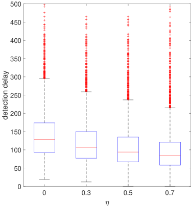
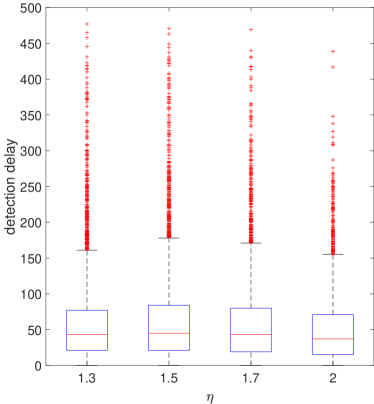
Figure 4.1. Boxplot of detection Delays when $m=500$, $\mathcal{n}=500$ for a change at $k^{*}=\lfloor\sqrt{\mathcal{n}}\rfloor$ under $H_{A,2}$. Left Panel: the monitoring procedure based on Theorem 3.1(i); Right Panel: the monitoring procedure based on Theorem 3.1(ii).

5. Empirical illustration

We illustrate our monitoring procedures using daily returns of individual stocks. We focus on four stocks: Apple Inc. (ticker: AAPL, Permno: 14593), Middlefield Banc Corp. (ticker: MBCN, Permno: 14932), Genetic Technologies Ltd (ticker: GENE, Permno: 90899), and NTS Realty Holdings LP (ticker: NLP, Permno: 90508). We download daily returns (without dividend) from the CRSP database. We consider two periods in order to showcase the detection for four types of changes (in the sense of the four different alternatives in our simulation). Depending on the specific purpose of the researcher, one can choose between the monitoring procedures based on Theorem 3.1(i) and (ii). Based on our simulations,if the aim is to quickly detect very early changes, we suggest using the Rényi type statistics based on Theorem 3.1(ii), with some tolerance for the compromise in size and power; conversely, if the purpose is to have good size control and high power, it is recommended to use the monitoring procedure based on Theorem 3.1(i). In this application, our preference is to have a good balance of size and power, and the procedure based on Theorem 3.1(i) (with the choice of $\eta=0.3$) delivers a good performance with sample sizes similar to the dataset used in this section. Before applying our monitoring procedure, it is necessary to ensure there is no change during the historical training sample. To this end, we use the test developed by Horváth and Wang (2024, labeled as HW(2024) hereinafter). Their test is to detect changes in GARCH(1,1) processes without assuming stationarity, which can accommodate either stationary or nonstationary historical sample. A rejection of their test indicates there is no change of $(\alpha,\beta)$ in the GARCH(1,1) during the historical sample. At the same time, we are keen to understand which the type of four changes may occur. Thus, we firstly examine whether our historical sample is stationary or not by employing the nonstationarity test developed by Francq and Zakoïan (2012, labeled as FZ(2012) hereinafter). At the end of our monitoring horizon, we use the FZ(2012) test again to check the stationarity of the samples after the change (if there is one).

5.1. Change from a stationary regime

To illustrate changepoint detection from a stationary regime, we choose the training period of 2016–2019 (1007 trading days) and the monitoring period of 2020–2021 (507 trading days). The training period is before the outbreak of COVID-19, while the monitoring period is in the pandemic. We apply our monitoring procedure for the stocks of AAPL and MBCN during this period. Table 5.1 (Columns 1 and 2) reports the results of the sequential monitoring procedure, as well as other information, including HW(2024) test, FZ(2012) test, and parameter estimates. HW(2024) test indicates that there is no parameter change during the training sample for AAPL and MBCN. The nonstationarity test of FZ(2012) indicates that they are both stationary during the training sample. Our sequential monitoring detects a change of AAPL on July 31st, 2020 and a change of MBCN on May 8th, 2020. Based on the FZ(2012) test for the sample after the change, we can conclude that AAPL experienced a change from a stationary to another stationary regime, while MBCN shifted from a stationary regime to a nonstationary one. Figure 5.1 contains returns series (upper panel) during the monitoring period and the detector versus the boundary function (lower panel).

Table 5.1. Monitoring results of the four stocks

	AAPL	MBCN	GENE	NLP
Training Sample
Start Date	2016-01-04	2016-01-04	2007-01-03	2007-01-03
End Date	2019-12-31	2019-12-31	2010-12-31	2010-12-31
Sample Size	1007	1007	1011	1011
HW(2024) Test
Test stat	1.469	1.351	1.179	1.088
Rejection	Not Rej.	Not Rej.	Not Rej.	Not Rej.
FZ(2012) NS Test
$p$-value	0.00%	0.00%	35.29%	33.81%
Stationary or not	Stationary	Stationary	Nonstationary	Nonstationary
Parameter estimates
$\hat{\alpha}_{0}$	0.135	0.183	0.287	0.099
$\hat{\beta}_{0}$	0.745	0.579	0.816	0.916
Monitoring Sample
Start Date	2020-01-02	2020-01-02	2011-01-03	2011-01-03
End Date	2021-12-31	2021-12-31	2012-12-31	2012-12-31
Sample Size	507	507	505	505
Our Sequential Monitoring
Rejection	Rej.	Rej.	Rej.	Rej.
Time of Change	2020-07-31	2020-05-08	2011-04-27	2012-09-04
After the change
FZ(2012) NS Test
$p$-value	0.00%	10.38%	0.00%	100.00%
Stationary or not	Stationary	Nonstationary	Stationary	Nonstationary
Parameter estimates
$\hat{\alpha}_{A}$	0.052	0.091	0.488	0.001
$\hat{\beta}_{A}$	0.935	0.913	0.528	1.053

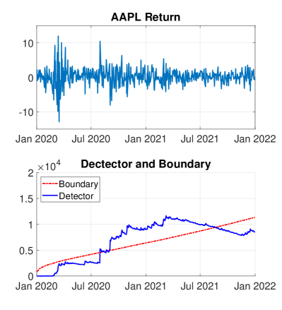
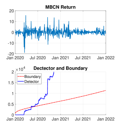
Figure 5.1. Upper Panel: the return series of AAPL (left) and MBCN (right) during the monitoring period; Lower Panel: the detector $\mathcal{D}_{m}(k)$ versus the boundary function $\mathfrak{g}_{m}(k)$ of AAPL (left) and MBCN (right).

5.2. Change from a nonstationary regime

We now consider detection from a nonstationary regime, and use 2007–2010 (1011 trading days) as the training period and 2011-2022 (505 trading days) as the monitoring period. The training period covers the global financial crisis (GFC), while the monitoring period follows the GFC but includes the European debt crisis. In this period, we monitor GENE and NLP. The results of the sequential monitoring procedure, alongside other supporting information, are displayed in Columns 3 and 4 of Table 5.1. Based on the HW(2024) test, we cannot reject that the return series of GENE and NLP have change in the training period. As evidenced by the nonstationarity test of FZ(2012), both stocks are in the nonstationary regime during the training period. Our sequential monitoring procedure reveals a change of GENE on April 27th, 2011 and a change of NLP on September 4th, 2012. After applying FZ(2012) nonstationarity test on the sample after the change, it is found that the change of GENE is from a nonstationary regime to a stationary regime, whilst the change of NLP is from a nonstationary to another nonstationary regime. It is also interesting to note that GENE after the change is in a strict stationary regime, but not in a second-order stationary regime. Figure 5.2 shows their returns series (upper panel) during the monitoring period and the detector versus the boundary function (lower panel).

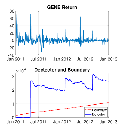
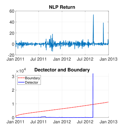
Figure 5.2. Upper Panel: the return series of GENE (left) and NLP (right) during the monitoring period; Lower Panel: the detector $\mathcal{D}_{m}(k)$ versus the boundary function $\mathfrak{g}_{m}(k)$ of GENE (left) and NLP (right).

6. Conclusions and discussions

In this paper, we complement the existing literature on (ex-ante) testing for bubble phenomena by proposing a family of weighted, CUSUM-based statistics to detect changes in the parameters of a GARCH(1,1) process. Our monitoring procedure can be applied irrespective of whether, in the training sample, the observations are stationary or explosive, and it is able to detect all types of changes: (a) from a stationary to another stationary regime (which is helpful in order to avoid the issues concerning the consistent estimation of a GARCH(1,1) process spelt out in Hillebrand, 2005); (b) from a stationary to an explosive regime (which contains information on the possible inception of a bubble); (c) from an explosive to a stationary regime (which, in the light of the previous point, could shed light on the cooling off the turbulence associated with a bubble on a financial market); and (d) from an explosive to another explosive regime (which, depending on the direction of the change - towards a more or a less explosive regime - could indicate whether exuberant volatility is heating up or cooling down). Technically, we propose two families of statistics, both based on weighted versions of the CUSUM process of the quasi-Fisher scores: one family uses lighter weights, and it is designed to detect, optimally, changes occurring not immediately after the start of the monitoring horizon; the other family uses heavier, Rényi-type weights, which make it more sensitive to changepoints occurring immediately after the end of the training period. For both cases, we study the limiting distribution of the detection delays; to the best of our knowledge, no such results exist for the case of a GARCH(1,1) models, and no results in general exist for the case of Rényi statistics. Given the interest in the detection of bubble phenomena, and the scant amount of contributions in the context of detection of changes in the volatility, we believe that our paper should be a useful addition to the toolbox of the financial econometrician.

A. Implementation guidelines, further Monte Carlo evidence, and further empirical results

A.1. Practical guidance on the implementation

In this section, we provide a detailed step-by-step guidance on implementing our sequential monitoring procedures (based on Theorem 3.1), which could be useful for researchers who want to apply it without studying the underlying theory. The steps are as follows:

1. Use QMLE to estimate the parameters $\boldsymbol{\theta}$ using the training sample

   $$\hat{\boldsymbol{\theta}}_{m}=\mbox{\rm argmax}\left\{\sum_{i=1}^{m}\bar{\ell}_{i}(\boldsymbol{\theta}):\;\boldsymbol{\theta}\in\boldsymbol{\Theta}\right\},$$

   where

   $$\bar{\ell}_{i}(\boldsymbol{\theta})=\log\bar{\sigma}_{i}^{2}+\dfrac{y_{i}^{2}}{\bar{\sigma}_{i}^{2}},$$

   and

   $$\bar{\sigma}_{i}^{2}(\boldsymbol{\theta})=\omega+\alpha y_{i-1}+\beta\bar{\sigma}_{i-1}^{2}(\boldsymbol{\theta}),\;\;\;\;\;1\leq i\leq m.$$

2. Calculate the quasi-Fisher scores of the log likelihood function

   $$\frac{\partial\bar{\ell}_{i}(\hat{\boldsymbol{\theta}}_{m})}{\partial\alpha}=\frac{\partial\bar{\ell}_{i}(\hat{\boldsymbol{\theta}}_{m})}{\partial\bar{\sigma}_{i}^{2}(\hat{\boldsymbol{\theta}}_{m})}\frac{\partial\bar{\sigma}_{i}^{2}(\hat{\boldsymbol{\theta}}_{m})}{\partial\alpha}=\frac{1}{\bar{\sigma}_{i}^{2}(\hat{\boldsymbol{\theta}}_{m})}\left(1-\frac{y_{i}^{2}}{\bar{\sigma}_{i}^{2}(\hat{\boldsymbol{\theta}}_{m})}\right)\frac{\partial\bar{\sigma}_{i}^{2}(\hat{\boldsymbol{\theta}}_{m})}{\partial\alpha},\;\;\;\;\;1\leq i\leq m+\mathcal{n},$$

   $$\frac{\partial\bar{\ell}_{i}(\hat{\boldsymbol{\theta}}_{m})}{\partial\beta}=\frac{\partial\bar{\ell}_{i}(\hat{\boldsymbol{\theta}}_{m})}{\partial\bar{\sigma}_{i}^{2}(\hat{\boldsymbol{\theta}}_{m})}\frac{\partial\bar{\sigma}_{i}^{2}(\hat{\boldsymbol{\theta}}_{m})}{\partial\beta}=\frac{1}{\bar{\sigma}_{i}^{2}(\hat{\boldsymbol{\theta}}_{m})}\left(1-\frac{y_{i}^{2}}{\bar{\sigma}_{i}^{2}(\hat{\boldsymbol{\theta}}_{m})}\right)\frac{\partial\bar{\sigma}_{i}^{2}(\hat{\boldsymbol{\theta}}_{m})}{\partial\beta},\;\;\;\;\;1\leq i\leq m+\mathcal{n}.$$

   To implement the above calculation, we need the following recursive equations:

   $$\frac{\partial\bar{\sigma}_{i}^{2}(\hat{\boldsymbol{\theta}}_{m})}{\partial\alpha}=y_{i-1}^{2}+\beta\frac{\partial\bar{\sigma}_{i-1}^{2}(\hat{\boldsymbol{\theta}}_{m})}{\partial\alpha},$$

   $$\frac{\partial\bar{\sigma}_{i}^{2}(\hat{\boldsymbol{\theta}}_{m})}{\partial\beta}=\bar{\sigma}_{i-1}^{2}(\hat{\boldsymbol{\theta}}_{m})+\beta\frac{\partial\bar{\sigma}_{i-1}^{2}(\hat{\boldsymbol{\theta}}_{m})}{\partial\beta},$$

   with initial values set to

   $$\frac{\partial\bar{\sigma}_{0}^{2}(\hat{\boldsymbol{\theta}}_{m})}{\partial\alpha}=\frac{\partial\bar{\sigma}_{0}^{2}(\hat{\boldsymbol{\theta}}_{m})}{\partial\beta}=0,$$

   which follows Fiorentini et al. (1996) and Pelagatti and Lisi (2009).

3. Estimate the covariance matrix of the derivatives in the training sample

   $$\hat{\mathbf{D}}_{m}=\dfrac{1}{m}\sum_{i=i}^{m}\left(\frac{\partial\bar{\ell}_{i}(\hat{\boldsymbol{\theta}}_{m})}{\partial\alpha},\frac{\partial\bar{\ell}_{i}(\hat{\boldsymbol{\theta}}_{m})}{\partial\beta}\right)^{\top}\left(\frac{\partial\bar{\ell}_{i}(\hat{\boldsymbol{\theta}}_{m})}{\partial\alpha},\frac{\partial\bar{\ell}_{i}(\hat{\boldsymbol{\theta}}_{m})}{\partial\beta}\right).$$

4. Obtain the detector

   $$\mathcal{D}_{m}(k)=\mathcal{r}_{m,k}^{\top}(\hat{\boldsymbol{\theta}}_{m})\hat{\mathbf{D}}_{m}^{-1}\mathcal{r}_{m,k}(\hat{\boldsymbol{\theta}}_{m}),\;\;\;\;\;m\leq k<m+\mathcal{n},$$

   where

   $$\mathcal{r}_{m,k}(\boldsymbol{\theta})=\sum_{i=m+1}^{m+k}\left(\frac{\partial\bar{\ell}_{i}(\boldsymbol{\theta})}{\partial\alpha},\frac{\partial\bar{\ell}_{i}(\boldsymbol{\theta})}{\partial\beta}\right)^{\top}.$$

5. Based on Theorem 3.1(i), a break is flagged as soon as the detector $\mathcal{D}_{m}(k)$ exceeds the tuned boundary function

   $$\mathfrak{g}_{m}(k)=\mathcal{c}\mathcal{n}\left(1+\dfrac{1}{\log(m)}\right)^{2}\left(1+\dfrac{k}{m}\right)^{2}\left(\dfrac{k}{\mathcal{n}}\right)^{\eta},\quad\;\;\mbox{where}\;\;1\leq k\leqslant\mathcal{n}-1;$$

   based on Theorem 3.1(ii), a break is indicated as soon as the detector $\mathcal{D}_{m}(k)$ goes above the tuned boundary function

   $$\bar{\mathfrak{g}}_{m}(k)=\mathcal{c}r\left(1+\dfrac{1}{\log(m)}\right)^{2}\left(1+\dfrac{k}{m}\right)^{2}\left(\frac{k}{r}\right)^{\eta},\quad\;\;\mbox{where}\;\;r\leq k\leqslant\mathcal{n}-1;$$

   otherwise, no break is reported.

A.2. Additional simulation results

Table A.1. Empirical size based on Theorem 3.1(ii)

		$\epsilon_{i}\sim\mathcal{N}(0,1)$				$\epsilon_{i}\sim$ Student’s $t$
		$m=500$	$m=1000$	$m=5000$		$m=500$	$m=1000$	$m=5000$
		Stationary GARCH(1,1)
		$\mathcal{n}=250$
$\tau=1.3$		14.2%	11.9%	9.4%		18.5%	13.8%	11.1%
$\tau=1.5$		12.4%	10.0%	7.7%		15.6%	11.4%	9.1%
$\tau=1.7$		11.0%	8.7%	6.9%		14.0%	10.0%	7.8%
$\tau=2.0$		9.4%	7.7%	5.8%		11.9%	8.7%	6.9%
		$\mathcal{n}=500$
$\tau=1.3$		14.8%	10.9%	8.8%		18.9%	15.2%	12.0%
$\tau=1.5$		12.8%	9.4%	7.1%		15.7%	12.9%	9.8%
$\tau=1.7$		11.2%	8.3%	6.3%		13.9%	11.6%	8.6%
$\tau=2.0$		10.0%	7.2%	5.4%		11.9%	10.0%	7.7%
		NonStationary GARCH(1,1)
		$\mathcal{n}=250$
$\tau=1.3$		13.8%	11.6%	10.1%		19.1%	14.5%	11.2%
$\tau=1.5$		11.4%	9.5%	8.5%		15.9%	12.1%	9.7%
$\tau=1.7$		10.4%	8.3%	7.6%		14.0%	10.9%	8.3%
$\tau=2.0$		8.7%	7.3%	6.6%		12.0%	9.5%	7.1%
		$\mathcal{n}=500$
$\tau=1.3$		13.3%	10.8%	9.7%		18.3%	14.2%	11.0%
$\tau=1.5$		11.8%	9.0%	8.3%		15.6%	12.4%	9.1%
$\tau=1.7$		10.5%	7.9%	7.3%		14.0%	10.7%	8.0%
$\tau=2.0$		9.1%	7.2%	6.6%		12.4%	9.5%	7.1%

Table A.2. Empirical power based on Theorem 3.1(ii) for a change at $k^{\ast}=\lfloor\sqrt{\mathcal{n}}\rfloor$

$\mathcal{n}=500$		$H_{A,1}$				$H_{A,2}$
before $k^{*}=\lfloor\sqrt{\mathcal{n}}\rfloor$		$\beta_{0}=0.80$				$\beta_{0}=0.80$
after $k^{*}=\lfloor\sqrt{\mathcal{n}}\rfloor$		$\beta_{1}=0.60$				$\beta_{1}=0.90$
$\epsilon_{i}\sim\mathcal{N}(0,1)$		$m=500$	$m=1000$	$m=5000$		$m=500$	$m=1000$	$m=5000$
$\eta=1.3$		83.18%	96.92%	100.00%		97.38%	100.00%	100.00%
$\eta=1.5$		61.78%	81.22%	99.62%		90.36%	98.68%	100.00%
$\eta=1.7$		41.70%	50.02%	83.42%		78.28%	92.08%	99.94%
$\eta=2.0$		23.40%	21.54%	21.56%		57.94%	65.18%	86.94%
$\epsilon_{i}\sim$ Student’s $t$
$\eta=1.3$		52.46%	71.82%	96.60%		90.46%	97.16%	99.88%
$\eta=1.5$		29.94%	37.48%	64.74%		82.34%	91.20%	99.06%
$\eta=1.7$		19.36%	16.00%	16.12%		72.08%	79.40%	93.50%
$\eta=2.0$		12.90%	8.98%	6.62%		55.80%	57.54%	62.86%
$\mathcal{n}=500$		$H_{A,3}$				$H_{A,4}$
before $k^{*}=\lfloor\sqrt{\mathcal{n}}\rfloor$		$\beta_{0}=0.90$				$\beta_{0}=0.90$
after $k^{*}=\lfloor\sqrt{\mathcal{n}}\rfloor$		$\beta_{1}=0.80$				$\beta_{1}=1.00$
$\epsilon_{i}\sim\mathcal{N}(0,1)$		$m=500$	$m=1000$	$m=5000$		$m=500$	$m=1000$	$m=5000$
$\eta=1.3$		100.00%	100.00%	100.00%		96.02%	99.78%	100.00%
$\eta=1.5$		99.88%	100.00%	100.00%		87.06%	97.58%	100.00%
$\eta=1.7$		99.48%	99.98%	100.00%		73.94%	86.94%	99.68%
$\eta=2.0$		97.04%	99.70%	100.00%		53.06%	57.54%	77.02%
$\epsilon_{i}\sim$ Student’s $t$
$\eta=1.3$		99.64%	99.98%	100.00%		86.36%	94.92%	99.70%
$\eta=1.5$		99.26%	99.86%	100.00%		75.78%	86.50%	97.92%
$\eta=1.7$		98.02%	99.76%	100.00%		64.62%	72.14%	87.64%
$\eta=2.0$		94.98%	98.28%	99.98%		48.70%	47.94%	50.70%

Table A.3. Empirical power based on Theorem 3.1(ii) for a change at $k^{\ast}=\lfloor 0.5\mathcal{n}\rfloor$

$\mathcal{n}=500$		$H_{A,1}$				$H_{A,2}$
before $k^{*}=\lfloor 0.5\mathcal{n}\rfloor$		$\beta_{0}=0.80$				$\beta_{0}=0.80$
after $k^{*}=\lfloor 0.5\mathcal{n}\rfloor$		$\beta_{1}=0.60$				$\beta_{1}=0.90$
$\epsilon_{i}\sim\mathcal{N}(0,1)$		$m=500$	$m=1000$	$m=5000$		$m=500$	$m=1000$	$m=5000$
$\eta=1.3$		21.96%	31.82%	68.10%		55.94%	74.74%	97.18%
$\eta=1.5$		13.38%	11.70%	20.02%		36.16%	48.14%	80.00%
$\eta=1.7$		11.08%	7.88%	7.00%		22.76%	24.90%	38.76%
$\eta=2.0$		9.34%	6.60%	5.90%		12.82%	9.52%	7.22%
$\epsilon_{i}\sim$ Student’s $t$
$\eta=1.3$		19.90%	17.22%	22.84%		54.20%	62.88%	79.52%
$\eta=1.5$		15.70%	11.72%	9.72%		39.02%	41.70%	52.72%
$\eta=1.7$		13.78%	9.82%	8.06%		27.32%	25.60%	24.78%
$\eta=2.0$		12.16%	8.30%	6.84%		16.74%	12.46%	8.14%
$\mathcal{n}=500$		$H_{A,3}$				$H_{A,4}$
before $k^{*}=\lfloor 0.5\mathcal{n}\rfloor$		$\beta_{0}=0.90$				$\beta_{0}=0.90$
after $k^{*}=\lfloor 0.5\mathcal{n}\rfloor$		$\beta_{1}=0.80$				$\beta_{1}=1.00$
$\epsilon_{i}\sim\mathcal{N}(0,1)$		$m=500$	$m=1000$	$m=5000$		$m=500$	$m=1000$	$m=5000$
$\eta=1.3$		96.20%	99.36%	99.98%		49.88%	66.64%	94.26%
$\eta=1.5$		91.46%	97.62%	99.78%		31.74%	38.80%	68.92%
$\eta=1.7$		82.48%	92.58%	98.96%		19.56%	18.66%	26.42%
$\eta=2.0$		64.50%	75.26%	91.88%		12.50%	9.26%	7.16%
$\epsilon_{i}\sim$ Student’s $t$
$\eta=1.3$		92.50%	97.56%	99.84%		44.16%	51.12%	71.38%
$\eta=1.5$		85.94%	93.78%	98.94%		30.78%	31.32%	39.32%
$\eta=1.7$		77.12%	86.66%	96.38%		21.04%	17.84%	15.50%
$\eta=2.0$		61.24%	68.16%	83.06%		14.72%	10.76%	7.32%

A.3. Further results - empirical application using Rényi weights

Figure A.1 presents the detector $\mathcal{D}_{m}(k)$ (with the choice of $\eta=1.5$) versus the boundary function $\bar{\mathfrak{g}}_{m}(k)$ based on Theorem 3.1 (ii) for the four stocks during the same periods analysed in Section 5. The monitoring procedure based on the Rényi type statistics detects a change of AAPL on March 2nd, 2020, a change of MBCN on March 13th, 2020, a change of GENE on April 27th, 2011, and a change of NLP on September 4th, 2012. Such results illustrate the merit of Rényi type statistics for the fast detection of very early changes, in particular for AAPL (nearly 5 months earlier) and MBCN (about 2 months earlier), compared to the procedure based on Theorem 3.1(i).

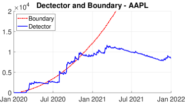
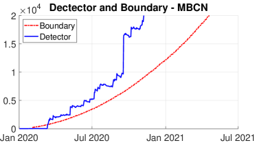
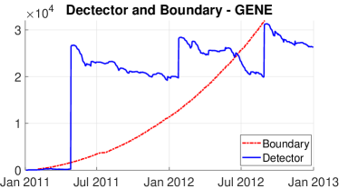
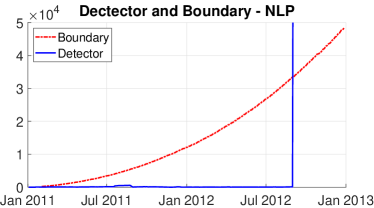
Figure A.1. The detector $\mathcal{D}_{m}(k)$ versus the boundary function $\bar{\mathfrak{g}}_{m}(k)$ based on Theorem 3.1 (ii)

B. Technical lemmas

Henceforth, we use $\nabla$ and $\nabla^{2}$ for the gradient vector and the Hessian matrix. We begin with some facts and notation which we will use throughout the proofs.

If (3.2) holds, then there is a unique, stationary, non anticipative sequence $\{x_{i},-\infty<i<\infty\}$ satisfying

$$x_{i}=h_{i}\epsilon_{i},\quad\;\;h_{i}^{2}=\omega_{0}+\alpha_{0}x_{i-1}^{2}+\beta_{0}h_{i-1}^{2},\quad\;\;-\infty<i<\infty$$

(cf. Berkes et al., 2003, and Francq and Zakoian, 2019). Next we define

$$\bar{h}_{i}^{2}(\mbox{\boldmath${\theta}$})=\omega+\alpha x_{i-1}^{2}+\beta\bar{h}_{i-1}^{2}(\mbox{\boldmath${\theta}$}),$$

$\mbox{\boldmath${\theta}$}=(\omega,\alpha,\beta)^{\top}$. The stationary version of the likelihood function is

$$\bar{f}_{i}(\mbox{\boldmath${\theta}$})=\log\bar{h}_{i}^{2}(\mbox{\boldmath${\theta}$})+\frac{x_{i}^{2}}{\bar{h}_{i}^{2}(\mbox{\boldmath${\theta}$})}$$

and we define

$${{\mathcal{f}}}_{k}(\mbox{\boldmath${\theta}$})=\sum_{i=1}^{k}\bar{f}_{i}(\mbox{\boldmath${\theta}$}).$$

Similarly, the stationary version of ${\mathcal{r}}_{m,k}(\mbox{\boldmath${\theta}$})$ is

(B.1) $$\bar{{\mathcal{r}}}_{m,k}(\mbox{\boldmath${\theta}$})=\sum_{i=m+1}^{m+k}\left(\frac{\partial\bar{f}_{i}(\mbox{\boldmath${\theta}$})}{\partial\alpha},\frac{\partial\bar{f}_{i}(\mbox{\boldmath${\theta}$})}{\partial\beta}\right)^{\top}.$$

Berkes et al. (2003) and Francq and Zakoian (2019) showed that the matrix

$${\mathbf{H}}=E\nabla^{2}\bar{f}_{0}(\mbox{\boldmath${\theta}$}_{0}),$$

exists and it is non singular.

After the change the observations are given by

(B.2) $$y_{i}=\sigma_{i}\epsilon_{i}\;\;\;\mbox{and}\;\;\;\sigma_{i}^{2}=\omega_{A}+\alpha_{A}y_{i-1}^{2}+\beta_{A}\sigma_{i-1}^{2},\;\;\;i>m+k^{\ast}.$$

Lemma B.1.

If Assumptions 2.1 and 2.2 hold, then we have

$$m\left(\hat{\mbox{\boldmath${\theta}$}}_{m}-\mbox{\boldmath${\theta}$}_{0}\right)=-{\mathbf{H}}^{-1}\nabla{{\mathcal{f}}}_{m}(\mbox{\boldmath${\theta}$}_{0})+O_{P}\left(\frac{1}{m}\right).$$

Proof.

The lemma is taken from Berkes et al. (2003) and Francq and Zakoian, 2019 (cf. also Lemma 5.3 in Horváth and Wang, 2024). ∎

Lemma B.2.

If Assumptions 2.1–2.3 hold, then we have

(B.3) $$\max_{1\leq k\leq{\mathcal{n}}}\frac{1}{k^{\zeta}}\sup_{\mbox{\boldmath${\theta}$}\in\mbox{\boldmath${\theta}$}}\left\|{\mathcal{r}}_{m,k}(\mbox{\boldmath${\theta}$})-\bar{{\mathcal{r}}}_{m,k}(\mbox{\boldmath${\theta}$})\right\|=O_{P}(1),$$

with some $\zeta<1/2$ and

(B.4) $$\max_{1\leq k\leq{\mathcal{n}}}\frac{1}{{\mathcal{n}}^{1/2}(k/{\mathcal{n}})^{\gamma}}\sup_{\mbox{\boldmath${\theta}$}\in\mbox{\boldmath${\theta}$}}\left\|{\mathcal{r}}_{m,k}(\mbox{\boldmath${\theta}$})-\bar{{\mathcal{r}}}_{m,k}(\mbox{\boldmath${\theta}$})\right\|=o_{P}(1),$$

for all $0\leq\gamma<1/2$.

Proof.

It is shown in Berkes et al. (2003), Francq and Zakoian (2004), and Francq and Zakoian (2019) that there is a constant $0<\rho<1$ such that

$$\sup_{\mbox{\boldmath${\theta}$}\in\mbox{\boldmath${\theta}$}}\left|\bar{\sigma}_{m+i}^{2}(\mbox{\boldmath${\theta}$})-\bar{h}_{m+i}^{2}(\mbox{\boldmath${\theta}$})\right|=O\left(\rho^{i}\right)\quad\quad a.s.$$

$$\sup_{\mbox{\boldmath${\theta}$}\in\mbox{\boldmath${\theta}$}}\left\|\nabla\bar{\sigma}_{m+i}^{2}(\mbox{\boldmath${\theta}$})-\nabla\bar{h}_{m+i}^{2}(\mbox{\boldmath${\theta}$})\right\|=O\left(\rho^{i}\right)\quad\quad a.s.$$

and

$$\left|y_{m+i}^{2}-x_{m+i}^{2}\right|=O\left(\rho^{i}\right)\quad\quad a.s.$$

Since $\underline{\omega}\leq\bar{\sigma}_{h}^{2}(\mbox{\boldmath${\theta}$})$ and $\underline{\omega}\leq\bar{h}_{j}^{2}(\mbox{\boldmath${\theta}$})$ for all $j\geq 1$, elementary calculations yield (B.3). Now (B.3) implies

$$\max_{1\leq k\leq{\mathcal{n}}}\frac{1}{{\mathcal{n}}^{1/2}(k/{\mathcal{n}})^{\gamma}}\sup_{\mbox{\boldmath${\theta}$}\in\mbox{\boldmath${\theta}$}}\left\|{\mathcal{r}}_{m,k}(\mbox{\boldmath${\theta}$})-\bar{{\mathcal{r}}}_{m,k}(\mbox{\boldmath${\theta}$})\right\|=O_{P}(1){\mathcal{n}}^{-1/2+\gamma}\max_{1\leq k\leq{\mathcal{n}}}k^{-\gamma+\zeta}=o_{P}(1).$$

∎

Lemma B.3.

If Assumptions 2.1–2.3 hold, then we have

$$\max_{1\leq k\leq{\mathcal{n}}}\frac{1}{{\mathcal{n}}^{1/2}(k/{\mathcal{n}})^{\gamma}}\left\|{\mathcal{r}}_{m,k}(\hat{\mbox{\boldmath${\theta}$}}_{m})-\bar{{\mathcal{r}}}_{m,k}(\mbox{\boldmath${\theta}$}_{0})\right\|=o_{P}(1),$$

for all $0\leq\gamma<1/2$.

Proof.

Lemma B.2 yields

$$\max_{1\leq k\leq{\mathcal{n}}}\frac{1}{{\mathcal{n}}^{1/2}(k/{\mathcal{n}})^{\gamma}}\sup_{\mbox{\boldmath${\theta}$}\in\mbox{\boldmath${\theta}$}}\left\|{\mathcal{r}}_{m,k}(\hat{\mbox{\boldmath${\theta}$}}_{m})-\bar{{\mathcal{r}}}_{m,k}(\hat{\mbox{\boldmath${\theta}$}}_{m})\right\|=o_{P}(1).$$

It is proven in Berkes et al. (2003) that there is a neighbourhood of $\mbox{\boldmath${\theta}$}_{0}$, say $\mbox{\boldmath${\theta}$}_{0}$, such that

$$\max_{1\leq k\leq{\mathcal{n}}}\sup_{\mbox{\boldmath${\theta}$}\in\mbox{\boldmath${\theta}$}_{0}}\frac{1}{k}\left\|\nabla^{3}{\mathcal{f}}_{m,k}(\mbox{\boldmath${\theta}$})\right\|=O_{P}(1).$$

Using a two term Taylor expansion coordinate-wise, we conclude that

(B.5) $$\nabla{\mathcal{f}}_{m,k}(\hat{\mbox{\boldmath${\theta}$}}_{m})-\nabla{\mathcal{f}}_{m,k}(\mbox{\boldmath${\theta}$}_{0})=\nabla^{2}{\mathcal{f}}_{m,k}(\mbox{\boldmath${\theta}$}_{0})(\hat{\mbox{\boldmath${\theta}$}}_{m}-\mbox{\boldmath${\theta}$}_{0})+\mathbf{R}_{m,k},$$

and

$$\max_{1\leq k\leq{\mathcal{n}}}\frac{1}{{\mathcal{n}}^{1/2}(k/{\mathcal{n}})^{\gamma}}\|\mathbf{R}_{m,k}\|=O_{P}({\mathcal{n}}^{1/2})\|\hat{\mbox{\boldmath${\theta}$}}_{m}-\mbox{\boldmath${\theta}$}_{0}\|^{2}.$$

The central limit for decomposable Bernoulli shifts (cf. Horváth and Wang, 2024) yields that

(B.6) $$\|\nabla{\mathcal{f}}_{m}(\mbox{\boldmath${\theta}$}_{0})\|=O_{P}\left(m^{1/2}\right),$$

and therefore Lemma B.1 and Assumption 2.3 give

(B.7) $$\max_{1\leq k\leq{\mathcal{n}}}\frac{1}{{\mathcal{n}}^{1/2}(k/{\mathcal{n}})^{\gamma}}\|\mathbf{R}_{m,k}\|=o_{P}(1).$$

According to the ergodic theorem (cf. Breiman, 1968)

(B.8) $$\max_{1\leq k\leq{\mathcal{n}}}\frac{1}{k}\left\|\nabla^{2}{\mathcal{f}}_{m,k}(\mbox{\boldmath${\theta}$}_{0})\right\|=O_{P}(1),$$

and therefore Lemma B.1 implies

$$\max_{1\leq k\leq{\mathcal{n}}}\frac{1}{{\mathcal{n}}^{1/2}(k/{\mathcal{n}})^{\gamma}}\left\|\nabla^{2}{\mathcal{f}}_{m}(\mbox{\boldmath${\theta}$}_{0})(\hat{\mbox{\boldmath${\theta}$}}_{m}-\mbox{\boldmath${\theta}$}_{0})\right\| =O_{P}\left(m^{-1/2}\right)\max_{1\leq k\leq{\mathcal{n}}}\frac{k}{{\mathcal{n}}^{1/2}(k/{\mathcal{n}})^{\gamma}}$$

$$=O_{P}\left(\left(\frac{{\mathcal{n}}}{m}\right)^{1/2}\right)=o_{P}(1).$$

Given that $\bar{{\mathcal{r}}}_{m,k}(\mbox{\boldmath${\theta}$})$ is made of the first two coordinates of $\nabla{\mathcal{f}}_{m,k}(\mbox{\boldmath${\theta}$})$, the proof is complete. ∎

Lemma B.4.

If Assumptions 2.1–2.3 hold, then, for any $m$, we can a define Gaussian process $\{\mbox{\boldmath${\Gamma}$}_{m}(t)\in R^{2},t\geq 0\}$ with $E\mbox{\boldmath${\Gamma}$}_{m}(t)=\mathbf{0}$ and $E\mbox{\boldmath${\Gamma}$}_{m}(t)\mbox{\boldmath${\Gamma}$}_{m}(s)=\min(t,s)\mathbf{D}$,

(B.9) $$\mathbf{D}=E\left[\left(\frac{\partial\bar{f}_{1}(\mbox{\boldmath${\theta}$}_{0})}{\partial\alpha},\frac{\partial\bar{f}_{1}(\mbox{\boldmath${\theta}$}_{0})}{\partial\beta}\right)^{\top}\left(\frac{\partial\bar{f}_{1}(\mbox{\boldmath${\theta}$}_{0})}{\partial\alpha},\frac{\partial\bar{f}_{1}(\mbox{\boldmath${\theta}$}_{0})}{\partial\beta}\right)\right],$$

such that for any $0\leq\gamma<1/2$

$$\max_{1\leq k\leq{\mathcal{n}}}\frac{1}{{\mathcal{n}}^{1/2}(k/{\mathcal{n}})^{\gamma}}\left\|\bar{{\mathcal{r}}}_{m,k}(\mbox{\boldmath${\theta}$}_{0})-\mbox{\boldmath${\Gamma}$}_{m}(k)\right\|=o_{P}(1),$$

Proof.

It is shown in Horváth and Wang (2024) that $\{\nabla{\mathcal{f}}_{m,k}(\mbox{\boldmath${\theta}$}_{0}),k\geq 1\}$ is a decomposable Bernoulli shift. Hence $\{\bar{{\mathcal{r}}}_{m,k}(\mbox{\boldmath${\theta}$}_{0}),k\geq 1\}$ is also a decomposable Bernoulli shift, and therefore by Lemma S2.1 of Aue et al. (2014) we can define Wiener processes $\mbox{\boldmath${\Gamma}$}_{m}(t)\in R^{2}$ with $E\mbox{\boldmath${\Gamma}$}_{m}(t)=\mathbf{0}$ and $E\mbox{\boldmath${\Gamma}$}_{m}(t)\mbox{\boldmath${\Gamma}$}_{m}(s)=\min(t,s)\mathbf{D}$ such that

(B.10) $$\sup_{1\leq k<\infty}\frac{1}{k^{\zeta}}\left\|\bar{{\mathcal{r}}}_{m,k}(\mbox{\boldmath${\theta}$}_{0})-\mbox{\boldmath${\Gamma}$}_{m}(k)\right\|=O_{P}(1),$$

with some $\zeta<1/2$. Since

$$\sup_{1\leq k\leq{\mathcal{n}}}\frac{k^{\zeta}}{{\mathcal{n}}^{1/2}(k/{\mathcal{n}})^{\gamma}}=o(1),$$

the result is proven. ∎

Lemma B.5.

If Assumptions 2.1–2.4 hold, then we have

(B.11) $$\max_{r\leq k\leq{\mathcal{n}}}\frac{1}{r^{1/2}(k/r)^{\gamma}}\sup_{\mbox{\boldmath${\theta}$}\in\mbox{\boldmath${\theta}$}}\left\|{\mathcal{r}}_{m,k}(\mbox{\boldmath${\theta}$})-\bar{{\mathcal{r}}}_{m,k}(\mbox{\boldmath${\theta}$})\right\|=o_{P}(1),$$

(B.12) $$\max_{r\leq k\leq{\mathcal{n}}}\frac{1}{r^{1/2}(k/r)^{\gamma}}\left\|\bar{{\mathcal{r}}}_{m,k}(\hat{\mbox{\boldmath${\theta}$}}_{m})-\bar{{\mathcal{r}}}_{m,k}(\mbox{\boldmath${\theta}$}_{0})\right\|=o_{P}(1),$$

and

(B.13) $$\max_{r\leq k\leq{\mathcal{n}}}\frac{1}{r^{1/2}(k/r)^{\gamma}}\left\|\bar{{\mathcal{r}}}_{m,k}(\mbox{\boldmath${\theta}$}_{0})-\mbox{\boldmath${\Gamma}$}_{m}(t)\right\|=o_{P}(1),$$

for all $\gamma>1/2$, where $\{\mbox{\boldmath${\Gamma}$}_{m}(t),t\geq 0\}$ is defined in Lemma B.4.

Proof.

It follows from (B.3) that

$$\max_{r\leq k\leq{\mathcal{n}}} \frac{1}{r^{1/2}(k/r)^{\gamma}}\sup_{\mbox{\boldmath${\theta}$}\in\mbox{\boldmath${\theta}$}}\left\|{\mathcal{r}}_{m,k}(\mbox{\boldmath${\theta}$})-\bar{{\mathcal{r}}}_{m,k}(\mbox{\boldmath${\theta}$})\right\|$$

$$=\max_{r\leq k\leq{\mathcal{n}}}\frac{k^{\zeta}}{r^{1/2}(k/r)^{\gamma}}\max_{1\leq k\leq{\mathcal{n}}}\sup_{\mbox{\boldmath${\theta}$}\in\mbox{\boldmath${\theta}$}}\frac{1}{k^{\zeta}}\left\|{\mathcal{r}}_{m,k}(\mbox{\boldmath${\theta}$})-\bar{{\mathcal{r}}}_{m,k}(\mbox{\boldmath${\theta}$})\right\|$$

$$=O_{P}\left(r^{\zeta-1/2}\right)=o_{P}(1),$$

since $r\rightarrow\infty$; hence (B.11) is proven. Turning to (B.12), the expansion in (B.5) implies

$$\max_{r\leq k\leq{\mathcal{n}}}\frac{1}{r^{1/2}(k/r)^{\gamma}}\|\mathbf{R}_{m,k}\| =\left\{\begin{array}[]{ll}O_{P}\left(({\mathcal{n}}/m)(r/{\mathcal{n}})^{\gamma}r^{-1/2}\right),\;\;\;\mbox{if}\;\;\;1/2<\gamma<1,\vspace{0.3cm}&\\ O_{P}\left(r^{1/2}/m\right),\;\;\;\mbox{if}\;\;\;\gamma\geq 1,&\end{array}\right.$$

$$=o_{P}(1).$$

Now Lemma B.1, (B.5) and (B.6) yield

$$\max_{r\leq k\leq{\mathcal{n}}}\frac{1}{r^{1/2}(k/r)^{\gamma}}\|\nabla\bar{{\mathcal{r}}}_{m,k}(\mbox{\boldmath${\theta}$}_{0})(\hat{\mbox{\boldmath${\theta}$}}_{m}-\mbox{\boldmath${\theta}$}_{0})\| =\left\{\begin{array}[]{ll}O_{P}\left(({\mathcal{n}}/m)(r/{\mathcal{n}})^{\gamma-1/2}\right),\;\;\;\mbox{if}\;\;\;1/2<\gamma<1\vspace{0.3cm}&\\ O_{P}\left((r/{\mathcal{n}})^{\gamma-1/2}({\mathcal{n}}/m)^{1/2}\right),\;\;\;\mbox{if}\;\;\;\gamma\geq 1&\end{array}\right.$$

$$=o_{P}(1),$$

completing the proof of (B.12). Finally, the approximation in (B.13) is an immediate consequence of Lemma B.4, since

$$\max_{r\leq k\leq{\mathcal{n}}}\frac{1}{r^{1/2}(k/r)^{\gamma}}\left\|\bar{{\mathcal{r}}}_{m,k}(\mbox{\boldmath${\theta}$}_{0})-\mbox{\boldmath${\Gamma}$}_{m}(t)\right\| \leq\max_{r\leq k\leq{\mathcal{n}}}\frac{k^{\zeta}}{r^{1/2}(k/r)^{\gamma}}\max_{1\leq k\leq{\mathcal{n}}}\frac{1}{k^{\zeta}}\left\|\bar{{\mathcal{r}}}_{m,k}(\mbox{\boldmath${\theta}$}_{0})-\mbox{\boldmath${\Gamma}$}_{m}(t)\right\|$$

$$=o_{P}(1).$$

∎

Lemma B.6.

If Assumptions 2.1 and 2.2 hold, then we have for all $1<\overline{\omega}$ there is $0<\rho<1$ such that

$$\sup_{1\leq i<\infty}\sup_{1/\overline{\omega}\leq\omega\leq\overline{\omega}}\frac{1}{\rho^{i}}|\bar{p}_{m+i,1}(\bar{\mbox{\boldmath${\theta}$}}_{0},\omega)-{\mathcal{z}}_{m+i,1}|=O_{P}(1)$$

and

$$\sup_{1\leq i<\infty}\sup_{1/\overline{\omega}\leq\omega\leq\overline{\omega}}\frac{1}{\rho^{i}}|\bar{p}_{m+i,2}(\bar{\mbox{\boldmath${\theta}$}}_{0},\omega)-{\mathcal{z}}_{m+i,2}|=O_{P}(1).$$

Proof.

Using the proofs from Jensen and Rahbek (2004), Horváth and Wang (2024) established the result as their Lemma 5.7. ∎

Lemma B.7.

We assume that Assumptions 2.1–2.3 hold.
(i) If $0\leq\gamma<1/2$, then we have

$$\max_{1\leq k\leq{\mathcal{n}}}\frac{1}{{\mathcal{n}}^{1/2}(k/{\mathcal{n}})^{\gamma}}\left\|{\mathcal{r}}_{m,k}(\hat{\mbox{\boldmath${\theta}$}}_{m})-\mathbf{q}_{m+k}\right\|=o_{P}(1).$$

(ii) If in addition, Assumption 2.4 also holds, and $\gamma>1/2$, then we have

$$\max_{r\leq k\leq{\mathcal{n}}}\frac{1}{r^{1/2}(k/r)^{\gamma}}\left\|{\mathcal{r}}_{m,k}(\hat{\mbox{\boldmath${\theta}$}}_{m})-\mathbf{q}_{m+k}\right\|=o_{P}(1).$$

Proof.

Let $\bar{\mbox{\boldmath${\theta}$}}_{0}=(\alpha_{0},\beta_{0})$. Jensen and Rahbek (2004) showed there is a neighbourhood of $\bar{\mbox{\boldmath${\theta}$}}_{0}$, say $\bar{\mbox{\boldmath${\theta}$}}_{0}$, such that

(B.14) $$\sup_{\underline{\omega}\leq\omega\leq\overline{\omega}}\sup_{(\alpha,\beta)\in\bar{\mbox{\boldmath${\theta}$}}_{0}}\frac{1}{k}\left\|\nabla{\mathcal{r}}_{m,k}(\alpha,\beta,\omega)\right\|=O_{P}(1).$$

Let $\bar{\mbox{\boldmath${\theta}$}}_{m}$ denote the vector of the first two coordinates of $\hat{\mbox{\boldmath${\theta}$}}_{m}$. Jensen and Rahbek (2004) proved that

(B.15) $$\sup_{\underline{\omega}\leq\omega\leq\overline{\omega}}\|\bar{\mbox{\boldmath${\theta}$}}_{m}-\bar{\mbox{\boldmath${\theta}$}}_{0}\|=O_{P}\left(m^{-1/2}\right)$$

(note that the estimator $\bar{\mbox{\boldmath${\theta}$}}_{m}$ might depend on $\omega)$. Using the mean value theorem coordinate–wise, we get from Lemma B.6 that

$$\|{\mathcal{r}}_{m,k}(\hat{\mbox{\boldmath${\theta}$}}_{m})-\mathbf{q}_{m+k}\|\leq\sup_{\underline{\omega}\leq\omega\leq\overline{\omega}}\sup_{(\alpha,\beta)\in\bar{\mbox{\boldmath${\theta}$}}_{0}}\left\|\nabla{\mathcal{r}}_{m,k}(\alpha,\beta,\omega)\right\|\|\bar{\mbox{\boldmath${\theta}$}}_{m}-\bar{\mbox{\boldmath${\theta}$}}_{0}\|^{1/2}$$

with probability tending to 1. Thus we get from (B.14) and (B.15) that

$$\max_{1\leq k\leq{\mathcal{n}}}\frac{1}{{\mathcal{n}}^{1/2}(k/{\mathcal{n}})^{\gamma}}\left\|{\mathcal{r}}_{m,k}(\hat{\mbox{\boldmath${\theta}$}}_{m})-\mathbf{q}_{m+k}\right\| =O_{P}\left(m^{-1/2}{\mathcal{n}}^{-1/2+\gamma}\max_{1\leq k\leq{\mathcal{n}}}k^{1-\gamma}\right)$$

$$=O_{P}\left(\left(\frac{{\mathcal{n}}}{m}\right)^{1/2}\right)=o_{P}(1).$$

Similarly,

$$\max_{r\leq k\leq{\mathcal{n}}} \frac{1}{r^{1/2}(k/r)^{\gamma}}\left\|{\mathcal{r}}_{m,k}(\hat{\mbox{\boldmath${\theta}$}}_{m})-\mathbf{q}_{m+k}\right\|$$

$$=O_{P}\left(m^{-1/2}r^{-1/2+\gamma}\max_{r\leq k\leq{\mathcal{n}}}k^{1-\gamma}\right)$$

$$=\left\{\begin{array}[]{ll}O_{P}\left(({\mathcal{n}}/m)^{1/2}(r/{\mathcal{n}})^{\gamma_{1}/2}\right),\quad\;\mbox{if}\;\;\;1/2<\gamma\leq 1\vspace{0.3cm}&\\ O_{P}\left(({\mathcal{n}}/m)^{1/2}\right),\quad\;\mbox{if}\;\;\;\gamma>1&\end{array}\right.$$

$$=o_{P}(1).$$

∎

Lemma B.8.

If Assumptions 2.1–2.3 hold, then for any $m$ we can define a Gaussian process $\{\mbox{\boldmath${\Gamma}$}_{m}(t),t\geq 0\}$, $E\mbox{\boldmath${\Gamma}$}_{m}(t)=\mathbf{0},E\mbox{\boldmath${\Gamma}$}_{m}(t)\mbox{\boldmath${\Gamma}$}_{m}(s)=\min(t,s)\mathbf{D}$ with

(B.16) $$\mathbf{D}=E[1-\epsilon_{m}^{2}]^{2}E\left[\left({\mathcal{z}}_{m,1},{\mathcal{z}}_{m,2}\right)^{\top}\left({\mathcal{z}}_{m,1},{\mathcal{z}}_{m,2}\right)\right].$$

such that
(i) if $0\leq\gamma<1/2$, then

(B.17) $$\max_{1\leq k\leq{\mathcal{n}}}\frac{1}{{\mathcal{n}}^{1/2}(k/{\mathcal{n}})^{\gamma}}\left\|\mathbf{q}_{m+k}-\mbox{\boldmath${\Gamma}$}_{m}(k)\right\|=o_{P}(1),$$

(ii) if in addition, Assumption 2.4 also holds and $\gamma>1/2$, then

(B.18) $$\max_{r\leq k\leq{\mathcal{n}}}\frac{1}{r^{1/2}(k/r)^{\gamma}}\left\|\mathbf{q}_{m+k}-\mbox{\boldmath${\Gamma}$}_{m}(k)\right\|=o_{P}(1).$$

Proof.

Horváth and Wang (2024) showed that $\{\mathbf{q}_{m+k},k\geq 1\}$ is a decomposable Bernoulli shift and therefore Lemma S2.1 of Aue et al. (2014) implies that for any $m$ there are Gaussian processes $\{\mbox{\boldmath${\Gamma}$}_{m}(k),k\geq 1\}$ such that

(B.19) $$\sup_{1\leq k<\infty}\frac{1}{k^{\zeta}}\left\|\mathbf{q}_{m+k}-\mbox{\boldmath${\Gamma}$}_{m}(k)\right\|=O_{P}(1)$$

with some $\zeta<1/2$, and $E\mbox{\boldmath${\Gamma}$}(t)=\mathbf{0},\;E\mbox{\boldmath${\Gamma}$}(t)\mbox{\boldmath${\Gamma}$}^{\top}(s)=\min(t,s)\mathbf{D}$ and $\mathbf{D}$ is defined in (B.16). The approximation in (B.19) implies both (B.17) and (B.18) in the same way as (B.10) implies Lemma B.4 and (B.13). ∎

Lemma B.9.

We assume that $H_{A}$, Assumptions 2.1–2.3 and 3.1 are satisfied.
(i) If $E\log(\alpha_{A}\epsilon_{0}^{2}+\beta_{A})<0$, then

$$\max_{1\leq k\leq k^{\ast}}\frac{{\mathcal{D}}_{m,k}}{g_{m}(k)}=O_{P}\left(\left(\frac{k^{\ast}}{{\mathcal{n}}}\right)^{1-\eta}\right).$$

(ii) If $E\log(\alpha_{A}\epsilon_{0}^{2}+\beta_{A})<0$, then

$$\max_{r\leq k\leq\max(r,k^{\ast})}\frac{{\mathcal{D}}_{m,k}}{\bar{g}_{m}(k)}=O_{P}\left(1\right).$$

Proof.

The lemma follows from the proof of Theorem 3.1. ∎

Next we assume that (3.9) holds. The observations are generated by (B.2) but in contrast to the previous case, the sequence is explosive and cannot be approximated with a stationary sequence. However, we can approximate the gradient of the log likelihood function with a stationary sequence, we need only minor modifications of the arguments used before. We use the following sequences to approximate the gradient vector of the log likelihood function when (B.2) holds for an explosive sequence:

$${\mathcal{v}}_{m+k^{\ast}+i,1}=\sum_{j=1}^{\infty}\epsilon_{m+k^{\ast}+i-j}^{2}\frac{1}{\beta_{A}}\sum_{k=1}^{j}\frac{\beta_{A}}{\alpha_{A}\epsilon_{m+k^{\ast}+i-k}^{2}+\beta_{A}}\quad\;$$

and

$${\mathcal{v}}_{m+k^{\ast}+i,2}=\sum_{j=1}^{\infty}\frac{1}{\beta_{A}}\sum_{k=1}^{j}\frac{\beta_{A}}{\alpha_{A}\epsilon_{m+k^{\ast}+i-k}^{2}+\beta_{A}}.$$

Let

$$\tilde{\mathbf{q}}_{m,k^{\ast},i}=\sum_{j=k^{\ast}+1}^{i}\left((1-\epsilon_{m+j}^{2}){\mathcal{v}}_{m+j,1},(1-\epsilon_{m+j}^{2}){\mathcal{v}}_{m+j,2}\right)^{\top}.$$

Lemma B.10.

If $H_{A}$, Assumptions 2.1–2.3, 3.1 are satisfied and $E\log(\alpha_{A}\epsilon_{0}^{2}+\beta_{A})>0$, then we have

$$\max_{k^{\ast}<i\leq{\mathcal{n}}}\frac{1}{(i-k^{\ast})^{\zeta}}\left\|[{\mathcal{r}}_{m,m+i}-{\mathcal{r}}_{m,m+k^{\ast}}]-(i-k^{\ast})\mbox{\boldmath${\Upsilon}$}-\tilde{\mathbf{q}}_{m,k^{\ast},i}\right\|=O_{P}(1),$$

with some $\zeta<1/2$.

Proof.

After the changepoint the observations change into an explosive sequence with parameter $\mbox{\boldmath${\theta}$}_{A}$, hence the proofs of Lemmas B.6 and B.7 can be repeated. ∎

Lemma B.11.

If $H_{A}$, Assumptions 2.1–2.3, 3.1 are satisfied and $E\log(\alpha_{A}\epsilon_{0}^{2}+\beta_{A})>0$, then we can define Gaussian processes $\left\{\tilde{\mbox{\boldmath${\Gamma}$}}_{m}(t),t\geq 0\right\}$ with $E\tilde{\mbox{\boldmath${\Gamma}$}}_{m}(t)=\mathbf{0},E\tilde{\mbox{\boldmath${\Gamma}$}}_{m}(t)\tilde{\mbox{\boldmath${\Gamma}$}}_{m}^{\top}(s)=\min(t,s)\mbox{\boldmath${\Sigma}$}_{2}$, where $\mbox{\boldmath${\Sigma}$}_{2}$ is defined in (3.10), such that

$$\max_{k^{\ast}<k\leq{\mathcal{n}}}\frac{1}{(k-k^{\ast})^{\zeta}}\left\|\tilde{\mathbf{q}}_{m,k^{\ast},i}-(i-k^{\ast})\mbox{\boldmath${\Upsilon}$}-\tilde{\mbox{\boldmath${\Gamma}$}}_{m}(i-k^{\ast})\right\|=O_{P}(1).$$

Proof.

The proof is the same as of that of Lemma B.8. ∎

C. Proofs

Proof of Theorem 3.1.

We begin by showing the theorem under stationarity. It follows from Lemmas B.2–B.4 that

$$\sup_{1\leq k\leq{\mathcal{n}}}\frac{1}{{\mathcal{n}}(k/{\mathcal{n}})^{\eta}}\left\|{\mathcal{r}}_{m,k}^{\top}(\hat{\mbox{\boldmath${\theta}$}}_{m})\mathbf{D}^{-1}{\mathcal{r}}_{m,k}(\hat{\mbox{\boldmath${\theta}$}}_{m})-\mbox{\boldmath${\Gamma}$}_{m}^{\top}(k)\mathbf{D}^{-1}\mbox{\boldmath${\Gamma}$}_{m}(k)\right\|=o_{P}(1).$$

The covariance structure of $\mbox{\boldmath${\Gamma}$}_{m}(k)$ implies that

$$\sup_{1\leq k\leq{\mathcal{n}}}\frac{1}{{\mathcal{n}}(k/{\mathcal{n}})^{\eta}}\left|\mbox{\boldmath${\Gamma}$}_{m}^{\top}(k)\mathbf{D}^{-1}\mbox{\boldmath${\Gamma}$}_{m}(k)\right|\overset{{\mathcal{D}}}{=}\sup_{1\leq k\leq{\mathcal{n}}}\frac{1}{{\mathcal{n}}(k/{\mathcal{n}})^{\eta}}\left\|\mathbf{W}(k)\right\|^{2},$$

where $\{\mathbf{W}(t),t\geq 0\}$ has independent coordinates, identically distributed Wiener processes. Using the the scale transformation and continuity of the Wiener process we conclude

$$\sup_{1\leq k\leq{\mathcal{n}}}\frac{1}{{\mathcal{n}}(k/{\mathcal{n}})^{\eta}}\left\|\mathbf{W}(k)\right\|^{2}\overset{{\mathcal{D}}}{=}\sup_{1/{\mathcal{n}}\leq k/{\mathcal{n}}\leq}\frac{1}{(k/{\mathcal{n}})^{\eta}}\left\|\mathbf{W}(k/{\mathcal{n}})\right\|^{2}\overset{{\mathcal{D}}}{\rightarrow}\sup_{0<t\leq}\frac{1}{t^{\eta}}\left\|\mathbf{W}(t)\right\|^{2}.$$

The proof of part (i) of the theorem is complete when (3.2) holds since

(C.1) $$\left\|\hat{\mathbf{D}}_{m}-\mathbf{D}\right\|=o_{P}\left(1\right),$$

with $\mathbf{D}$ defined in (B.9). We now turn to proving the second part of the Theorem. We note

$$\max_{r\leq k\leq{\mathcal{n}}}\frac{1}{r(k/r)^{\eta}}\mbox{\boldmath${\Gamma}$}_{m}^{\top}(k)\mathbf{D}^{-1}\mbox{\boldmath${\Gamma}$}_{m}(k) \overset{{\mathcal{D}}}{=}\max_{r\leq k\leq{\mathcal{n}}}\frac{1}{r(k/r)^{\eta}}\left\|\mathbf{W}(k)\right\|^{2}$$

$$\overset{{\mathcal{D}}}{=}\max_{1\leq k/r\leq{\mathcal{n}}/r}\frac{1}{(k/r)^{\eta}}\left\|\mathbf{W}(k/r)\right\|^{2}$$

$$\overset{{\mathcal{D}}}{\rightarrow}\max_{1\leq t<\infty}\frac{1}{t^{\eta}}\left\|\mathbf{W}(t)\right\|^{2}$$

due to the almost sure continuity of the Wiener process, and the Law of the Iterated Logarithm for Wiener processes. The result in part (ii) of the theorem now follows from Lemma B.5 and (C.1). Under nonstationarity, the proof is exactly the same as above, only Lemmas B.2–B.5 are replaced with Lemmas B.6–B.8. We also note that according to Jensen and Rahbek (2004) (cf. also Francq and Zakoian, 2019), it holds that $\left\|\hat{\mathbf{D}}_{m}-\mathbf{D}\right\|=o_{P}(1)$, where $\mathbf{D}$ is defined in (B.16), thus completing the proof. ∎

Proof of Theorem 3.2.

We note that under our conditions, it holds that $\|\hat{\mathbf{D}}_{m}-\mathbf{D}\|=O_{P}(m^{-\delta})$, for some $\delta>0$. Hence in the proofs we can replace $\hat{\mathbf{D}}_{m}^{-1}$ with $\mathbf{D}^{-1}$ in the definition of the detector, without loss of generality. We wish to point out that the definition of $\mathbf{D}$ depends on the sign of $E\log(\alpha_{0}\epsilon_{0}^{2}+\beta_{0})$.
First we assume that $E\log(\alpha_{A}\epsilon_{0}^{2}+\beta_{A})<0$ holds. To prove part (i) of the theorem, we note that according to Lemma B.2

(C.2) $$\max_{1\leq k\leq{\mathcal{n}}}\frac{1}{k^{1/2}}\sup_{\mbox{\boldmath${\theta}$}\in\mbox{\boldmath${\theta}$}}\|{\mathcal{r}}_{m,k}(\mbox{\boldmath${\theta}$})-\bar{{\mathcal{r}}}_{m,k}(\mbox{\boldmath${\theta}$})\|=O_{P}(1),$$

and

(C.3) $$\max_{a\leq k\leq{\mathcal{n}}}\frac{1}{k^{1/2}}\sup_{\mbox{\boldmath${\theta}$}\in\mbox{\boldmath${\theta}$}}\|{\mathcal{r}}_{m,k}(\mbox{\boldmath${\theta}$})-\bar{{\mathcal{r}}}_{m,k}(\mbox{\boldmath${\theta}$})\|=O_{P}\left(a^{-1/2+\zeta}\right),$$

where $\zeta<1/2$ and $a=(\log{\mathcal{n}})^{\phi}$ with $\phi>4$. Following the proof of Lemma B.3 we get

$$\max_{1\leq k\leq{\mathcal{n}}}\frac{1}{k^{1/2}}\|\mathbf{R}_{m,k}\|=O_{P}({\mathcal{n}}^{1/2})\|\hat{\mbox{\boldmath${\theta}$}}_{m}-\mbox{\boldmath${\theta}$}_{0}\|^{2}=O_{P}\left(\frac{{\mathcal{n}}^{1/2}}{m}\right),$$

and by (B.7)

$$\max_{1\leq k\leq{\mathcal{n}}}\frac{1}{k^{1/2}}\left\|\nabla^{2}{\mathcal{f}}_{m,k}(\mbox{\boldmath${\theta}$}_{0})(\hat{\mbox{\boldmath${\theta}$}}_{m}-\mbox{\boldmath${\theta}$})\right\|=O_{P}\left(\frac{{\mathcal{n}}^{1/2}}{m^{1/2}}\right),$$

$$\max_{a\leq k\leq{\mathcal{n}}}\frac{1}{k^{1/2}}\left\|\nabla^{2}{\mathcal{f}}_{m,k}(\mbox{\boldmath${\theta}$}_{0})(\hat{\mbox{\boldmath${\theta}$}}_{m}-\mbox{\boldmath${\theta}$})\right\|=O_{P}\left(\frac{a^{1/2}}{m^{1/2}}\right).$$

Using the approximation in (B.10) we conclude

(C.4) $$\max_{1\leq k\leq{\mathcal{n}}}\frac{1}{k^{1/2}}\left\|\bar{{\mathcal{r}}}_{m,k}(\mbox{\boldmath${\theta}$}_{0})-\mbox{\boldmath${\Gamma}$}_{m}(k)\right\|=O_{P}\left(1\right)$$

and

(C.5) $$\max_{1\leq k\leq a}\frac{1}{k^{1/2}}\left\|\bar{{\mathcal{r}}}_{m,k}(\mbox{\boldmath${\theta}$}_{0})-\mbox{\boldmath${\Gamma}$}_{m}(k)\right\|=O_{P}\left(a^{-1/2+\zeta}\right).$$

The Darling–Erdős (cf. Csörgő and Horváth, 1997, pp. 363–365) yields

$$\frac{1}{2\log\log{\mathcal{n}}}\max_{1\leq k\leq{\mathcal{n}}}\frac{1}{k}\mbox{\boldmath${\Gamma}$}_{m}^{\top}(k)\mathbf{D}^{-1}\mbox{\boldmath${\Gamma}$}_{m}(k)\overset{P}{\rightarrow}1,$$

and

$$\max_{a\leq k\leq{\mathcal{n}}}\frac{1}{k}\mbox{\boldmath${\Gamma}$}_{m}^{\top}(k)\mathbf{D}^{-1}\mbox{\boldmath${\Gamma}$}_{m}(k)=O_{P}\left(\log\log\log{\mathcal{n}}\right).$$

Thus we obtain that

$$\lim_{m\rightarrow\infty}P\left\{\max_{1\leq k\leq{\mathcal{n}}}\frac{1}{k}{\mathcal{r}}_{m,k}^{\top}(\hat{\mbox{\boldmath${\theta}$}}_{m})\mathbf{D}^{-1}{\mathcal{r}}_{m,k}(\hat{\mbox{\boldmath${\theta}$}}_{m})=\max_{a\leq k\leq{\mathcal{n}}}\frac{1}{k}{\mathcal{r}}_{m,k}^{\top}(\hat{\mbox{\boldmath${\theta}$}}_{m})\mathbf{D}^{-1}{\mathcal{r}}_{m,k}(\hat{\mbox{\boldmath${\theta}$}}_{m})\right\}=1.$$

Putting together our estimates on the set $a\leq k\leq{\mathcal{n}}$, we get

$$\max_{a\leq k\leq{\mathcal{n}}}\frac{1}{k}\left|{\mathcal{r}}_{m,k}^{\top}(\hat{\mbox{\boldmath${\theta}$}}_{m})\mathbf{D}^{-1}{\mathcal{r}}_{m,k}(\hat{\mbox{\boldmath${\theta}$}}_{m})-\mbox{\boldmath${\Gamma}$}_{m}^{\top}(k)\mathbf{D}^{-1}\mbox{\boldmath${\Gamma}$}_{m}(k)\right|=O_{P}\left((\log{\mathcal{n}})^{-\bar{\phi}}\right),$$

with some $\bar{\phi}>0$. Since

$$\max_{a\leq k\leq{\mathcal{n}}}\mbox{\boldmath${\Gamma}$}_{m}^{\top}(k)\mathbf{D}^{-1}\mbox{\boldmath${\Gamma}$}_{m}(k)\overset{{\mathcal{D}}}{=}\max_{a\leq k\leq{\mathcal{n}}}\|\mathbf{W}(k)\|^{2},$$

where $\{\mathbf{W}(t),t\geq 0\}$ is defined in Theorem 3.1. Using Appendix 3 in Csörgő and Horváth (1997), we obtain that

$$\lim_{{\mathcal{n}}\rightarrow\infty}P\left\{a(\log{\mathcal{n}})\max_{a\leq k\leq{\mathcal{n}}}\|\mathbf{W}(k)\|\leq x+b_{2}(\log{\mathcal{n}})\right\}=\exp(-e^{-x})$$

for all $x$. Hence the proof Theorem 3.2(i) is complete when $E\log(\alpha_{0}\epsilon_{0}^{2}+\beta_{0})<0$.
Lemma B.6, (B.14) and (B.15) imply that (C.2) and (C.3) can be replaced with

$$\max_{1\leq k\leq{\mathcal{n}}}\frac{1}{k^{1/2}}\left\|{\mathcal{r}}_{m,k}(\hat{\mbox{\boldmath${\theta}$}}_{m})-\mathbf{q}_{m+k}\right\|=O_{P}(1),$$

and

$$\max_{a\leq k\leq{\mathcal{n}}}\frac{1}{k^{1/2}}\left\|{\mathcal{r}}_{m,k}(\hat{\mbox{\boldmath${\theta}$}}_{m})-\mathbf{q}_{m+k}\right\|=O_{P}(a^{-1/2+\zeta}),$$

with some $\zeta<1/2$, when $E\log(\alpha_{0}\epsilon_{0}^{2}+\beta_{0})>0$. The approximation in (B.19) yields

(C.6) $$\max_{1\leq k\leq{\mathcal{n}}}\frac{1}{k^{1/2}}\left\|\mathbf{q}_{m+k}-\mbox{\boldmath${\Gamma}$}_{m}(k)\right\|=O_{P}(1),$$

and

(C.7) $$\max_{a\leq k\leq{\mathcal{n}}}\frac{1}{k^{1/2}}\left\|\mathbf{q}_{m+k}-\mbox{\boldmath${\Gamma}$}_{m}(k)\right\|=O_{P}(a^{-1/2+\zeta}).$$

The approximations in (C.6) and (C.7) imply part (i) of the theorem, in the same way as (C.4) and (C.5) yielded (C.7) under condition $E\log(\alpha_{0}\epsilon_{0}^{2}+\beta_{0})<0$.
To prove part (ii) of the theorem, we use again the approximations in (C.4) and (C.5). By the scale transformation of Wiener processes we have

(C.8) $$\sup_{r\leq t\leq{\mathcal{n}}}\frac{1}{t^{1/2}}\|\mathbf{W}(t)\|\overset{{\mathcal{D}}}{=}\sup_{1\leq t\leq{\mathcal{n}}/r}\frac{1}{t^{1/2}}\|\mathbf{W}(t)\|$$

and therefore the Darling–Erdős limit result (cf. Csörgő and Horváth, 1997, pp. 363–368) with (C.4) and (C.5) yields

$$\frac{1}{2\log\log({\mathcal{n}}/r)}\max_{r\leq k\leq{\mathcal{n}}}\frac{1}{k}{\mathcal{r}}_{m,k}^{\top}(\hat{\mbox{\boldmath${\theta}$}}_{m})\mathbf{D}^{-1}{\mathcal{r}}_{m,k}\overset{P}{\rightarrow}1$$

and

$$\max_{r\leq k\leq rg}\frac{1}{k}{\mathcal{r}}_{m,k}^{\top}(\hat{\mbox{\boldmath${\theta}$}}_{m})\mathbf{D}^{-1}{\mathcal{r}}_{m,k}=O_{P}\left(\log\log\log({\mathcal{n}}/r)\right)$$

with

$$g=(\log({\mathcal{n}}/r))^{\bar{\phi}},\;\;\;\bar{\phi}>4.$$

Now we get

$$\lim_{m\rightarrow\infty}P\left\{\max_{r\leq k\leq{\mathcal{n}}}\frac{1}{k}{\mathcal{r}}_{m,k}^{\top}(\hat{\mbox{\boldmath${\theta}$}}_{m})\mathbf{D}^{-1}{\mathcal{r}}_{m,k}=\max_{rg\leq k\leq{\mathcal{n}}}\frac{1}{k}{\mathcal{r}}_{m,k}^{\top}(\hat{\mbox{\boldmath${\theta}$}}_{m})\mathbf{D}^{-1}{\mathcal{r}}_{m,k}\right\}=1.$$

Using the approximation of ${\mathcal{r}}_{m,k}(\hat{\mbox{\boldmath${\theta}$}}_{m})$ with Gaussian processes we get

$$\max_{rg\leq k\leq{\mathcal{n}}}\frac{1}{k}\left|{\mathcal{r}}_{m,k}^{\top}(\hat{\mbox{\boldmath${\theta}$}}_{m})\mathbf{D}^{-1}{\mathcal{r}}_{m,k}-\mbox{\boldmath${\Gamma}$}_{m}^{\top}(k)\mathbf{D}^{-1}\mbox{\boldmath${\Gamma}$}_{m}(k)\right|=O_{P}\left((\log({\mathcal{n}}/r))^{-\bar{\phi}}\right)$$

with some $\bar{\phi}>0$. Now using the results on pp. 363–365 in Csörgő and Horváth (1997) with (C.8) yields

$$\lim_{m\rightarrow\infty}P\left\{a(\log({\mathcal{n}}/r))\max_{rg\leq k\leq{\mathcal{n}}}\frac{1}{k^{1/2}}\left(\mbox{\boldmath${\Gamma}$}_{m}^{\top}(k)\mathbf{D}^{-1}\mbox{\boldmath${\Gamma}$}_{m}(k)\right)^{1/2}\leq x+b_{2}(\log({\mathcal{n}}/r))\right\}=\exp(-e^{-x}),$$

completing the proof of part (ii) of the theorem when $E\log(\alpha_{0}\epsilon_{0}^{2}+\beta_{0})<0$. The same arguments can be used when $E\log(\alpha_{0}\epsilon_{0}^{2}+\beta_{0})>0$. ∎

Proof of Theorem 3.3.

First we assume that (3.2) holds. After $m+k^{\ast}$, the sequence can turn into (asymptotically) stationary sequence. Since (3.2) holds, we have

$$\max_{k^{\ast}+1\leq j<\infty}\sup_{\mbox{\boldmath${\theta}$}\in\mbox{\boldmath${\theta}$}}\frac{1}{j-k^{\ast}}\|{\mathcal{r}}_{m,j}(\mbox{\boldmath${\theta}$})-{\mathcal{r}}_{m,k^{\ast}}(\mbox{\boldmath${\theta}$})-(j-k^{\ast}){\mathcal{r}}^{(1)}(\mbox{\boldmath${\theta}$})\|=o_{P}(1),$$

where

$${\mathcal{r}}^{(1)}(\mbox{\boldmath${\theta}$})=E\bar{{\mathcal{r}}}_{m,k^{\ast}+1}^{(1)}(\mbox{\boldmath${\theta}$}),$$

$$\bar{{\mathcal{r}}}_{m,k^{\ast}+j}^{(1)}(\mbox{\boldmath${\theta}$})=\sum_{i=k^{\ast}+1}^{k^{\ast}+j}\left(\frac{\partial\hat{\ell}_{i}(\mbox{\boldmath${\theta}$})}{\partial\alpha},\frac{\partial\hat{\ell}_{i}(\mbox{\boldmath${\theta}$})}{\partial\beta}\right)^{\top},$$

Under $H_{A}$ we have that $\mbox{\boldmath${\Delta}$}={\mathcal{r}}^{(1)}(\mbox{\boldmath${\theta}$}_{0})\neq\mathbf{0}.$ Next we write for $k>k^{\ast}$

(C.9) $${\mathcal{r}}_{m,k}(\hat{\mbox{\boldmath${\theta}$}}_{m})=(k-k^{\ast})\mbox{\boldmath${\Delta}$}+\mathbf{m}_{m,k}$$

with

(C.10) $$\mathbf{m}_{m,k}={\mathcal{r}}_{m,k^{\ast}}(\hat{\mbox{\boldmath${\theta}$}}_{m})+[{\mathcal{r}}_{m,k}(\hat{\mbox{\boldmath${\theta}$}}_{m})-{\mathcal{r}}_{m,k^{\ast}}(\hat{\mbox{\boldmath${\theta}$}}_{m})-(k-k^{\ast})\mbox{\boldmath${\Delta}$}]$$

We use the decomposition

(C.11) $${\mathcal{D}}_{m,k}=(k-k^{\ast})^{2}A_{m}+2(k-k^{\ast})\mbox{\boldmath${\Delta}$}^{\top}\hat{\mathbf{D}}_{m}^{-1}\mathbf{m}_{m,k}+\mathbf{m}_{m,k}^{\top}\mathbf{D}_{m}^{-1}\mathbf{m}_{m,k},$$

where $A_{m}$ is defined in (3.4). We note that, for any ${\mathcal{M}}$

$$\max_{1\leq k\leq{\mathcal{M}}}\frac{{\mathcal{D}}_{m,k}}{g_{m}(k)}=\max\left(\max_{1\leq k\leq k^{\ast}}\frac{{\mathcal{D}}_{m,k}}{g_{m}(k)},\max_{k^{\ast}+1\leq k\leq{\mathcal{M}}}\frac{{\mathcal{D}}_{m,k}}{g_{m}(k)}\right).$$

First we consider the case when (3.2) holds. The observations $y_{i}$ can be approximated with a stationary sequence defined in (3.3). Recalling the definitions of $t^{\ast},\bar{u},u_{{\mathcal{n}}}$ and $u^{\ast}$ in (3.6)–(3.8), we define

$${\mathcal{M}}=k^{\ast}+u_{{\mathcal{n}}}\left({\mathcal{n}}^{1-\eta}\frac{{\mathcal{c}}}{A_{m}}\right)^{1/(2-\eta)}+R,$$

with

$$R=x{(u^{\ast}+t^{\ast})^{3/2}}\left(\left({\mathcal{n}}^{1-\eta}\frac{{\mathcal{c}}}{A_{m}}\right)^{1/(2-\tau)}\right)^{1/2}.$$

Now according to Theorem 3.1

$$\left(\max_{1\leq k\leq k^{\ast}}\frac{{\mathcal{D}}_{m,k}}{k^{\eta}}-{\mathcal{c}}{\mathcal{n}}^{1-\eta}\right)\left({\mathcal{n}}^{(1-\eta)/(2-\eta)}\right)^{-3/2+\eta}\overset{\mathcal{P}}{\rightarrow}-\infty.$$

It follows from the proof of Theorem 3.1

$$\max_{k^{\ast}+1\leq k\leq{\mathcal{M}}}\frac{\mathbf{m}_{m,k}^{\top}\mathbf{D}_{m}^{-1}\mathbf{m}_{m,k}}{g_{m}(k)}=O_{P}(1),$$

and for any $\bar{\eta}<1/2$

$$\max_{k^{\ast}+1\leq k\leq{\mathcal{M}}}\frac{1}{k-k^{\ast}}\frac{\|\mathbf{m}_{m,k}\|}{{\mathcal{n}}^{1/2}(k/{\mathcal{n}})^{\bar{\eta}}}=O_{P}(1).$$

Let $0<\delta<1$ and write

$${\mathcal{n}}^{1-\eta}\max_{k^{\ast}+1\leq k\leq(1-\delta){\mathcal{M}}}\frac{{\mathcal{D}}_{m,k}}{g_{m}(k)}=(1-\delta)^{2-\eta}{\mathcal{M}}^{2-\eta}O_{P}(1),$$

where $O_{P}(1)$ does not depend on $\delta$. Thus we conclude

$$\left({\mathcal{n}}^{1-\eta}\max_{k^{\ast}+1\leq k\leq(1-\delta){\mathcal{M}}}\frac{{\mathcal{D}}_{m,k}}{g_{m}(k)}-{\mathcal{n}}^{1-\eta}\right)({\mathcal{n}}^{1-\eta})^{(-3/2+\eta)/(2-\eta)}\overset{\mathcal{P}}{\rightarrow}-\infty.$$

Our calculations show that we need to consider the asymptotic properties of

$$\left(\max_{(1-\delta){\mathcal{M}}\leq k\leq{\mathcal{M}}}\frac{1}{k^{\eta}}\left((k-k^{\ast})^{2}A_{m}+2(k-k^{\ast})\mbox{\boldmath${\Delta}$}^{\top}\hat{\mathbf{D}}_{m}^{-1}\mathbf{m}_{m,k}\right)\right.$$

$$\left.-\left[{\mathcal{c}}{\mathcal{n}}^{1-\eta}-\frac{1}{{\mathcal{M}}^{\eta}}({\mathcal{M}}-k^{\ast})^{2}A_{m}\right]\right)\left({\mathcal{n}}^{(1-\eta)/(2-\eta)}\right)^{-3/2+\eta}.$$

Since the model is the same until $y_{m+k^{\ast}}$, the $k^{\ast}$th observation following the training sample, we have that

(C.12) $$\mathbf{D}=\lim_{k^{\ast}\rightarrow\infty} \frac{1}{m+k^{\ast}}E\left\{\left(\frac{\partial\bar{{\mathcal{r}}}_{m,m+k^{\ast}}(\mbox{\boldmath${\theta}$}_{0})}{\partial\alpha},\frac{\partial\bar{{\mathcal{r}}}_{m,m+k^{\ast}}(\mbox{\boldmath${\theta}$}_{0})}{\partial\beta}\right)^{\top}\right.$$

$$\left.\hskip 85.35826pt\times\left(\frac{\partial\bar{{\mathcal{r}}}_{m,m+k^{\ast}}(\mbox{\boldmath${\theta}$}_{0})}{\partial\alpha},\frac{\partial\bar{{\mathcal{r}}}_{m,m+k^{\ast}}(\mbox{\boldmath${\theta}$}_{0})}{\partial\beta}\right)\right\}.$$

(Note that the formula for $\mathbf{D}$ depends on whether the training sample is stationary or non stationary, cf. Berkes et al., 2003 and Jensen and Rahbek, 2004). Along the lines of the proof of Theorem 3.1 one can show that

(C.13) $${\mathcal{M}}^{-3/2}\left(\lfloor{\mathcal{M}}t\rfloor-\lfloor k^{\ast}/{\mathcal{M}}\rfloor\right)\mbox{\boldmath${\Delta}$}^{\top}\hat{\mathbf{D}}_{m}^{-1}\mathbf{m}_{m,{\mathcal{M}}t}\overset{{\mathcal{D}}[1-\delta,1]}{\longrightarrow}(t-t^{\ast}/(u^{\ast}+t^{\ast}))Z(t),$$

where $\{Z(t),t\geq t^{\ast}/(t^{\ast}+u^{\ast})\}$ is a Gaussian process with $EZ(t)=0$ and

$$EZ(t)Z(s)=t^{\ast}\mbox{\boldmath${\Delta}$}^{\top}\mathbf{D}^{-1}\mbox{\boldmath${\Delta}$}+[\min(t,s)-t^{\ast}/(t^{\ast}+u^{\ast})]\mbox{\boldmath${\Delta}$}^{\top}\mathbf{D}^{-1}\mbox{\boldmath${\Sigma}$}_{1}\mathbf{D}^{-1}\mbox{\boldmath${\Delta}$},$$

where $\mbox{\boldmath${\Sigma}$}_{1}$ is defined in (3.5). Hence

$${\mathcal{M}}^{-1/2+\eta}\max_{(1-\delta){\mathcal{M}}\leq k\leq{\mathcal{M}}}\frac{1}{k^{\tau}}(k-k^{\ast})\mbox{\boldmath${\Delta}$}^{\top}\hat{\mathbf{D}}_{m}^{-1}\mathbf{m}_{m,k}\overset{{\mathcal{D}}}{\rightarrow}\sup_{1-\delta\leq t\leq 1}\frac{1}{t^{\eta}}(t-t^{\ast})Z(t).$$

Also, for any $x>0$

$$\lim_{\delta\rightarrow 0}\limsup_{m\rightarrow\infty} P\left\{{\mathcal{M}}^{-1/2+\eta}\max_{(1-\delta){\mathcal{M}}\leq k\leq{\mathcal{M}}}\frac{1}{k^{\eta}}\left|(k-k^{\ast})\mbox{\boldmath${\Delta}$}^{\top}\hat{\mathbf{D}}_{m}^{-1}\mathbf{m}_{m,k}-k^{\ast}\mbox{\boldmath${\Delta}$}^{\top}\hat{\mathbf{D}}_{m}^{-1}\mathbf{m}_{m,{\mathcal{M}}}\right|>x\right\}$$

$$=0.$$

Since $(k-k^{\ast})^{2}/t^{\eta}$ is increasing on $[(1-\delta){\mathcal{M}},{\mathcal{M}}]$ we get that

$$\lim_{\delta\rightarrow 0}\limsup_{m\rightarrow\infty}P\left\{\sup_{(1-\delta){\mathcal{M}}\leq k\leq{\mathcal{M}}}\frac{1}{k^{\eta}}\left((k-k^{\ast})^{2}A_{m}+2(k-k^{\ast})\mbox{\boldmath${\Delta}$}^{\top}\hat{\mathbf{D}}_{m}^{-1}\mathbf{m}_{m,k}\right)\right.$$

$$\left.=\frac{1}{{\mathcal{M}}^{\eta}}\left[({\mathcal{M}}-k^{\ast})^{2}A_{m}+2({\mathcal{M}}-k^{\ast})\mbox{\boldmath${\Delta}$}^{\top}\hat{\mathbf{D}}_{m}^{-1}\mathbf{m}_{m,{\mathcal{M}}}\right]\right\}=1.$$

Next we write

$$P \left\{\frac{1}{{\mathcal{M}}^{\eta}}\left[({\mathcal{M}}-k^{\ast})^{2}A_{m}+2({\mathcal{M}}-k^{\ast})\mbox{\boldmath${\Delta}$}^{\top}\hat{\mathbf{D}}_{m}^{-1}\mathbf{m}_{m,{\mathcal{M}}}\right]\leq{\mathcal{c}}{\mathcal{n}}^{1-\eta}\right\}$$

$$=P\left\{2({\mathcal{M}}-k^{\ast})[\mbox{\boldmath${\Delta}$}^{\top}\hat{\mathbf{D}}_{m}^{-1}\mathbf{m}_{m,{\mathcal{M}}}]{\mathcal{M}}^{-3/2}\leq\left[{\mathcal{c}}{\mathcal{n}}^{1-\eta}-\frac{1}{{\mathcal{M}}^{\eta}}({\mathcal{M}}-k^{\ast})^{2}A_{m}\right]{\mathcal{M}}^{-3/2+\eta}\right\}.$$

Using (C.13) we get

$${\mathcal{M}}^{-1/2}\mbox{\boldmath${\Delta}$}^{\top}\hat{\mathbf{D}}_{m}^{-1}\mathbf{m}_{m,{\mathcal{M}}}\overset{{\mathcal{D}}}{\rightarrow}\bar{s}_{1}{\mathcal{N}},$$

where ${\mathcal{N}}$ denotes a standard normal random variable, $\bar{s}_{1}$ is defined in (3.13) and $\mathbf{D}$ is the covariance matrix in (C.12). Also,

$$\left[{\mathcal{n}}^{1-\eta}-\frac{1}{{\mathcal{M}}^{\eta}}({\mathcal{M}}-k^{\ast})^{2}A_{m}\right]{\mathcal{M}}^{-3/2+\eta}\rightarrow-2x,$$

and thus we conclude

$$\lim_{m\rightarrow\infty} P\left\{2({\mathcal{M}}-k^{\ast})[\mbox{\boldmath${\Delta}$}^{\top}\hat{\mathbf{D}}_{m}^{-1}\mathbf{m}_{m,{\mathcal{M}}}]{\mathcal{M}}^{-3/2}\leq\left[{\mathcal{c}}{\mathcal{n}}^{1-\eta}-\frac{1}{{\mathcal{M}}^{\eta}}({\mathcal{M}}-k^{\ast})^{2}A_{m}\right]{\mathcal{M}}^{-3/2+\eta}\right\}$$

$$=P\left\{\bar{s}_{1}{\mathcal{N}}\leq-x\right\}=1-\Phi(x/\bar{s}_{1}).$$

We assume now that $t^{\ast}=\infty$ and $\bar{u}=0$ also holds. We modify the definition of ${\mathcal{M}}$ as

$${\mathcal{M}}=k^{\ast}+\left(\frac{{\mathcal{c}}}{A_{m}}{\mathcal{n}}^{1-\eta}(k^{\ast})^{\eta}\right)^{1/2}+R\quad\;\mbox{with}\quad\;R=\frac{x}{A_{m}}(k^{\ast})^{1/2}.$$

Proceeding as in the previous case we get that for any $0<\delta<1$

(C.14) $$\lim_{m\rightarrow\infty} P\left\{\tau_{m}>{\mathcal{M}}\right\}$$

$$=\lim_{m\rightarrow\infty}\left\{\max_{(1-\delta){\mathcal{M}}\leq k\leq{\mathcal{M}}}\frac{1}{k^{\eta}}\left((k-k^{\ast})^{2}A_{m}+2(k-k^{\ast})\mbox{\boldmath${\Delta}$}^{\top}\hat{\mathbf{D}}_{m}^{-1}\mathbf{m}_{m.k}\right)\leq{\mathcal{c}}{\mathcal{n}}^{1-\eta}\right\}$$

$$=\lim_{m\rightarrow\infty}P\left\{2({\mathcal{M}}-k^{\ast})\mbox{\boldmath${\Delta}$}^{\top}\hat{\mathbf{D}}_{m}^{-1}\mathbf{m}_{m,{\mathcal{M}}}\leq\left({\mathcal{c}}{\mathcal{n}}^{1-\eta}-\frac{1}{{\mathcal{M}}^{\eta}}({\mathcal{M}}-k^{\ast})^{2}A_{m}\right){\mathcal{M}}^{\eta}\right\}$$

$$=\lim_{m\rightarrow\infty}P\left\{2(k^{\ast})^{-1/2}\mbox{\boldmath${\Delta}$}^{\top}\hat{\mathbf{D}}_{m}^{-1}\mathbf{m}_{m,{\mathcal{M}}}\leq\left({\mathcal{c}}{\mathcal{n}}^{1-\eta}-\frac{1}{{\mathcal{M}}^{\tau}}({\mathcal{M}}-k^{\ast})^{2}A_{m}\right)\frac{{\mathcal{M}}^{\eta}}{({\mathcal{M}}-k^{\ast})(k^{\ast})^{1/2}}\right\}.$$

Using the definitions of ${\mathcal{M}}$ and $R$ we have

$$\left({\mathcal{c}}{\mathcal{n}}^{1-\eta}-\frac{1}{{\mathcal{M}}^{\eta}}({\mathcal{M}}-k^{\ast})^{2}A_{m}\right)\frac{{\mathcal{M}}^{\eta}}{({\mathcal{M}}-k^{\ast})(k^{\ast})^{1/2}}\rightarrow-2x.$$

As in the proof of (C.13) we have

$$(k^{\ast})^{-1/2}\mbox{\boldmath${\Delta}$}^{\top}\hat{\mathbf{D}}_{m}^{-1}\mathbf{m}_{m,{\mathcal{M}}}\overset{{\mathcal{D}}}{\rightarrow}\bar{s}_{2}{\mathcal{N}},$$

where ${\mathcal{N}}$ is a standard normal random variable and $\bar{s}_{2}$ is defined in (3.14). Now we conclude

$$\lim_{m\rightarrow\infty}P\{\tau_{m}>{\mathcal{M}}\}=1-\Phi(x/\bar{s}_{2}),$$

where $\Phi$ is the standard normal distribution function.
In the final case we write

$$k^{\ast}=u_{m}{\mathcal{n}}\;\;\;\;\mbox{with}\;\;\;u_{m}\rightarrow\bar{u}\in(0,1).$$

In this case, we define

$${\mathcal{M}}=k^{\ast}+x(k^{\ast})^{1/2}.$$

We write

$$\max_{1\leq k\leq{\mathcal{M}}}\frac{{\mathcal{D}}_{m,k}}{{\mathcal{n}}(k/{\mathcal{n}})^{\eta}}=\max\left(U_{1,m},U_{2,m}\right),$$

$$U_{1,m}=\max_{1\leq k\leq k^{\ast}}\frac{{\mathcal{D}}_{m,k}}{{\mathcal{n}}(k/{\mathcal{n}})^{\eta}}$$

and

$$U_{2,m}=\max_{k^{\ast}+1\leq k\leq{\mathcal{M}}}\frac{{\mathcal{D}}_{m,k}}{{\mathcal{n}}(k/{\mathcal{n}})^{\eta}}.$$

We use the decomposition in (C.10) and we note

$$\left(\frac{1}{k^{\ast}}\right)^{1/2}\max_{k^{\ast}+1\leq k\leq{\mathcal{M}}}\|{\mathcal{r}}_{m,k}(\hat{\mbox{\boldmath${\theta}$}}_{m})-{\mathcal{r}}_{m,k^{\ast}}(\hat{\mbox{\boldmath${\theta}$}}_{m})\|=O_{P}(1).$$

It follows from the proof of Theorem 3.1 that

$$\left(\max_{1\leq k\leq k^{\ast}}\frac{{\mathcal{D}}_{m,k}}{k^{\ast}(k/k^{\ast})^{\eta}},\left(\frac{1}{k^{\ast}}\right)^{1/2}{\mathcal{r}}_{m,k^{\ast}}(\hat{\mbox{\boldmath${\theta}$}}_{m})\right)\overset{{\mathcal{D}}}{\rightarrow}\left(\sup_{0\leq s\leq 1}\frac{\mbox{\boldmath${\Gamma}$}(s)^{\top}\mathbf{D}^{-1}\mbox{\boldmath${\Gamma}$}(s)}{s^{\eta}},\mbox{\boldmath${\Gamma}$}(1)\right),$$

where $\{\mbox{\boldmath${\Gamma}$}(s),s\geq 0\}$ is a Gaussian process with $E\mbox{\boldmath${\Gamma}$}(s)=\mathbf{0}$ and $E\mbox{\boldmath${\Gamma}$}(s)\mbox{\boldmath${\Gamma}$}^{\top}(t)=\min(t,s)\mathbf{D}.$ We write

$$U_{2,m}=\max_{1\leq j\leq x(k^{\ast})^{1/2}}\left(\frac{k^{\ast}+j}{m}\right)^{1-\eta}\left({\mathcal{r}}_{m,k^{\ast}}+j\mbox{\boldmath${\Delta}$}+[{\mathcal{r}}_{m,k^{\ast}}-{\mathcal{r}}_{m,k}]\right)^{\top}\hat{\mathbf{D}}_{m}^{-1}\left({\mathcal{r}}_{m,k^{\ast}}+j\mbox{\boldmath${\Delta}$}+[{\mathcal{r}}_{m,k^{\ast}}-{\mathcal{r}}_{m,k}]\right)^{\top}.$$

Thus we get

$$\left(U_{m,1},U_{m,2}\right)\overset{{\mathcal{D}}}{\rightarrow}\left(\sup_{0<t\leq 1}\frac{\bar{u}^{1-\eta}}{t^{\eta}}\mbox{\boldmath${\Gamma}$}^{\top}\mathbf{D}^{-1}\mbox{\boldmath${\Gamma}$}(t),\bar{u}^{1-\eta}\sup_{0\leq t\leq x}(t\mbox{\boldmath${\Delta}$}+\mbox{\boldmath${\Gamma}$}(1))^{\top}\mathbf{D}^{-1}(t\mbox{\boldmath${\Delta}$}+\mbox{\boldmath${\Gamma}$}(1))\right).$$

Next we assume that (3.9) holds. We replace (C.10) and (C.11) with

$${\mathcal{r}}_{m,k}(\hat{\mbox{\boldmath${\theta}$}}_{m})=(k-k^{\ast})\mbox{\boldmath${\Upsilon}$}+\tilde{\mathbf{m}}_{m,k},$$

$$\tilde{\mathbf{m}}_{m,k}={\mathcal{r}}_{m,k^{\ast}}(\hat{\mbox{\boldmath${\theta}$}}_{m})+[{\mathcal{r}}_{m,k}(\hat{\mbox{\boldmath${\theta}$}}_{m})-{\mathcal{r}}_{m,k^{\ast}}(\hat{\mbox{\boldmath${\theta}$}}_{m})-(k-k^{\ast})\mbox{\boldmath${\Upsilon}$}],$$

$${\mathcal{D}}_{m,k}=(k-k^{\ast})^{2}B_{m}+2(k-k^{\ast})\mbox{\boldmath${\Upsilon}$}^{\top}\hat{\mathbf{D}}_{m}^{-1}\tilde{\mathbf{m}}_{m,k}+\tilde{\mathbf{m}}_{m,k}^{\top}\hat{\mathbf{D}}_{m}^{-1}\tilde{\mathbf{m}}_{m,k}.$$

Following the same arguments as in the case of (3.2), we get that if $\bar{u}=0$, then

$$\lim_{m\rightarrow\infty}P\{\tau_{m}>\tilde{{\mathcal{M}}}\}$$

$$=\lim_{m\rightarrow\infty}P\left\{2(\tilde{{\mathcal{M}}}-k^{\ast})[\mbox{\boldmath${\Upsilon}$}^{\top}\hat{\mathbf{D}}_{m}^{-1}\tilde{\mathbf{m}}_{m,\tilde{{\mathcal{M}}}}]\tilde{{\mathcal{M}}}^{-3/2}\leq\left[{\mathcal{c}}{\mathcal{n}}^{1-\eta}-\frac{1}{\tilde{{\mathcal{M}}}^{\eta}}\left(\tilde{{\mathcal{M}}}-k^{\ast}\right)^{2}B_{m}\right]\tilde{{\mathcal{M}}}^{-3/2+\eta}\right\},$$

and the definition of $\tilde{{\mathcal{M}}}$ depends on if $\tilde{t}^{\ast}<\infty$ is finite or not. If $\tilde{t^{\ast}}<\infty$ we use

$$\tilde{{\mathcal{M}}}=k^{\ast}+\tilde{u}_{{\mathcal{n}}}\left({\mathcal{n}}^{1-\eta}\frac{{\mathcal{c}}}{B_{m}}\right)^{1/(2-\eta)}+\tilde{R},$$

with

$$\tilde{R}=x{(\tilde{u}^{\ast}+\tilde{t}^{\ast})^{3/2}}\left(\left({\mathcal{n}}^{1-\eta}\frac{{\mathcal{c}}}{B_{m}}\right)^{1/(2-\eta)}\right)^{1/2}.$$

Using the definition of $\bar{{\mathcal{M}}}$ we get

(C.15) $$\lim_{m\rightarrow\infty}\left[{\mathcal{c}}{\mathcal{n}}^{1-\tau}-\frac{1}{\tilde{{\mathcal{M}}}^{\tau}}\left(\tilde{{\mathcal{M}}}-k^{\ast}\right)^{2}B_{m}\right]\tilde{{\mathcal{M}}}^{-3/2+\tau}=-2x.$$

Applying (B.19) and Lemma B.10 with the independence of the approximating Gaussian processes we conclude

(C.16) $$(\tilde{{\mathcal{M}}}-k^{\ast})[\mbox{\boldmath${\Upsilon}$}^{\top}\hat{\mathbf{D}}_{m}^{-1}\tilde{\mathbf{m}}_{m,\tilde{{\mathcal{M}}}}]\tilde{{\mathcal{M}}}^{-3/2}\overset{{\mathcal{D}}}{\rightarrow}\bar{s}_{1}{\mathcal{N}},$$

where ${\mathcal{N}}$ is a standard normal random variable and $\bar{s}_{1}$ is defined in (3.13). The covariance matrix $\mathbf{D}$ is defined in (C.12). If $\tilde{t}^{\ast}=\infty$ and $\bar{u}=0$, then we use

$${\mathcal{M}}=k^{\ast}+\left(\frac{{\mathcal{c}}}{B_{m}}{\mathcal{n}}^{1-\eta}(k^{\ast})^{\eta}\right)^{1/2}+\tilde{R},\quad\;\mbox{with}\quad\;\tilde{R}=\frac{x}{B_{m}}(k^{\ast})^{1/2}.$$

We still have (C.15) but (C.16) is replaced with

$$(\tilde{{\mathcal{M}}}-k^{\ast})[\mbox{\boldmath${\Upsilon}$}^{\top}\hat{\mathbf{D}}_{m}^{-1}\tilde{\mathbf{m}}_{m,\tilde{{\mathcal{M}}}}]\tilde{{\mathcal{M}}}^{-3/2}\overset{{\mathcal{D}}}{\rightarrow}\bar{s}_{2}{\mathcal{N}},$$

where $\bar{s}_{2}$ is given in (3.14). As in the previous case, if $0<\bar{u}<1$, then we use again ${\mathcal{M}}=k^{\ast}+x(k^{\ast})^{1/2}$. Since the sum of gradients (after removing the mean) of the log likelihood function of the observations after the change is negligible, we get that

$$\max_{1\leq k\leq{\mathcal{M}}}\frac{{\mathcal{D}}_{m}(k)}{g_{m}(k)}\overset{{\mathcal{D}}}{\rightarrow}\bar{u}^{1-\eta}\max\left(\sup_{0<t\leq 1}\frac{1}{t^{\eta}}\mbox{\boldmath${\Gamma}$}^{\top}(t)\mathbf{D}^{-1}\mbox{\boldmath${\Gamma}$}(t),\sup_{0\leq t\leq x}(t\mbox{\boldmath${\Upsilon}$}+\mbox{\boldmath${\Gamma}$}(1)^{\top}\mathbf{D}^{-1}(t\mbox{\boldmath${\Upsilon}$}+\mbox{\boldmath${\Gamma}$}(t))\right),$$

where recall that $\{\mbox{\boldmath${\Gamma}$}(t),t\geq 0\}$ is a Gaussian process $E\mbox{\boldmath${\Gamma}$}(t)=\mathbf{0}$ and $E\mbox{\boldmath${\Gamma}$}(t)\mbox{\boldmath${\Gamma}$}^{\top}(s)=\min(t,s)\mathbf{D}$.

Next we consider the Rényi type detector. First we investigate the case when after the change we have an (asymptotically) stationary sequence. Assume that $k^{\ast}\leq r$, i.e. the change occurred before the monitoring started. By definition,

$$P\{\bar{\tau}_{m}=r\}=P\left\{\frac{{\mathcal{D}}_{m}(r)}{\bar{g}_{m}(r)}\geq 1\right\}.$$

The proof is based again on (C.9) and (C.10). It follows from Lemma B.9 that

$$\frac{1}{(k^{\ast})^{1/2}}\|{\mathcal{r}}_{m,k^{\ast}}\|=O_{P}(1)$$

and if $k^{\ast}\rightarrow\infty$ and $r-k^{\ast}\rightarrow\infty$, then

$$\left(\frac{1}{(k^{\ast})^{1/2}}{\mathcal{r}}_{m,k^{\ast}},\frac{1}{(r-k^{\ast})^{1/2}}\left[{\mathcal{r}}_{m,r}(\hat{\mbox{\boldmath${\theta}$}}_{m})-{\mathcal{r}}_{m,k^{\ast}}(\hat{\mbox{\boldmath${\theta}$}}_{m})-(r-k^{\ast})\mbox{\boldmath${\Delta}$}\right]\right)\overset{{\mathcal{D}}}{\rightarrow}\left(\mathbf{N}_{1},\mathbf{N}_{2}\right)$$

where $\mathbf{N}_{1},\mathbf{N}_{2}$ are independent standard normal random variables with covariance matrices $\mbox{\boldmath${\Sigma}$}_{1}$ and $\mbox{\boldmath${\Sigma}$}_{2}$ defined in (3.5) and (3.10), respectively. Thus we get

$$\frac{1}{r^{1/2}}\left((r-k^{\ast})\mbox{\boldmath${\Delta}$}+\mathbf{m}_{m,r}\right)\overset{{\mathcal{D}}}{\rightarrow}{\mathcal{a}}^{1/2}\mathbf{N}_{1}+{\mathcal{b}}+\mathbf{N}_{2}.$$

If ${\mathcal{a}}<\infty$, then we use

$${\mathcal{M}}=k^{\ast}+xr^{1/2}.$$

It follows from the proof of Theorem 3.1 that for all $K>0$

$$\left\{\frac{1}{r^{1/2}}{\mathcal{r}}_{m,rt}(\hat{\mbox{\boldmath${\theta}$}}_{m}),\frac{1}{r^{1/2}}\left({\mathcal{r}}_{m,k^{\ast}}+[{\mathcal{r}}_{m,xr^{1/2}}-{\mathcal{r}}_{m,k^{\ast}}-xr^{1/2}]\right),t\geq 0,x\geq 0\right\}$$

$$\hskip 56.9055pt\overset{{\mathcal{D}}[0,{\mathcal{a}}]\times[0,K]}{\longrightarrow}\left\{\mbox{\boldmath${\Gamma}$}_{1}(t),\mbox{\boldmath${\Gamma}$}_{1}({\mathcal{a}})+x\mbox{\boldmath${\Delta}$}\right\}$$

where $\{\mbox{\boldmath${\Gamma}$}_{1}(t),t\geq 0\}$ is Gaussian process with $E\mbox{\boldmath${\Gamma}$}_{1}(t)=\mathbf{0}$, $E\mbox{\boldmath${\Gamma}$}_{1}(t)\mbox{\boldmath${\Gamma}$}_{1}^{\top}(s)=\min(t,s)\mbox{\boldmath${\Sigma}$}_{1}$ with $\mbox{\boldmath${\Sigma}$}_{1}$ defined in (3.5). Thus we conclude

$$\sup_{r\leq k\leq{\mathcal{M}}} \frac{{\mathcal{D}}_{m}(k)}{g_{m}(k)}=\frac{1}{{\mathcal{c}}}\max\left(\max_{r\leq k\leq k^{\ast}}\frac{{\mathcal{D}}_{m}(k)}{(k/r)^{\eta}r},\;\max_{k^{\ast}<k\leq{\mathcal{M}}}\frac{{\mathcal{D}}_{m}(k)}{(k/r)^{\eta}r}\right)$$

$$\overset{{\mathcal{D}}}{\rightarrow}\frac{1}{{\mathcal{c}}{\mathcal{a}}^{\eta}}\max\left(\sup_{1\leq t\leq{\mathcal{a}}}\mbox{\boldmath${\Gamma}$}_{1}^{\top}(t)\mathbf{D}^{-1}\mbox{\boldmath${\Gamma}$}_{1}(t),\;\max_{0\leq s\leq x}(\mbox{\boldmath${\Gamma}$}_{1}({\mathcal{a}})+s\mbox{\boldmath${\Delta}$})^{\top}\mathbf{D}^{-1}(\mbox{\boldmath${\Gamma}$}_{1}({\mathcal{a}})+s\mbox{\boldmath${\Delta}$}).\right).$$

For the final case ${\mathcal{a}}=\infty$ we use

$${\mathcal{M}}=k^{\ast}+\left(\frac{{\mathcal{c}}}{A_{m}}\frac{(k^{\ast})^{\eta}}{r^{\eta-1}}\right)^{1/2}+x(k^{\ast})^{1/2}.$$

We observe that

(C.17) $$\frac{k^{\ast}}{((k^{\ast})^{\eta}/r^{\eta-1})^{1/2}}=\left(\left(\frac{k^{\ast}}{r}\right)^{2-\eta}r\right)^{1/2}\rightarrow\infty$$

and

(C.18) $$\frac{(k^{\ast})^{\eta}/r^{\eta-1}}{k^{\ast}}=\left(\frac{k^{\ast}}{r}\right)^{\eta-1}\rightarrow\infty.$$

As in the previous cases,

$$\lim_{m\rightarrow\infty} P\{\bar{\tau}_{m}>{\mathcal{M}}\}$$

$$=\lim_{m\rightarrow\infty}P\left\{2({\mathcal{M}}-k^{\ast})\mbox{\boldmath${\Delta}$}^{\top}\hat{\mathbf{D}}_{m}^{-1}\mathbf{m}_{m,{\mathcal{M}}}<\left[{\mathcal{c}}r^{1-\eta}-\frac{({\mathcal{M}}-k^{\ast})^{2}A_{m}}{{\mathcal{M}}^{\eta}}\right]{\mathcal{M}}^{\eta}\right\}$$

$$=\lim_{m\rightarrow\infty}P\left\{2{\mathcal{M}}^{-1/2}\mbox{\boldmath${\Delta}$}^{\top}\hat{\mathbf{D}}_{m}^{-1}\mathbf{m}_{m,{\mathcal{M}}}<\left[{\mathcal{c}}r^{1-\eta}-\frac{({\mathcal{M}}-k^{\ast})^{2}A_{m}}{{\mathcal{M}}^{\eta}}\right]\frac{1}{{\mathcal{M}}-k^{\ast}}{\mathcal{M}}^{-1/2+\eta}\right\}.$$

We obtain from (C.17) and (C.18) that

$$\left[{\mathcal{c}}r^{1-\eta}-\frac{({\mathcal{M}}-k^{\ast})^{2}A_{m}}{{\mathcal{M}}^{\eta}}\right]\frac{1}{{\mathcal{M}}-k^{\ast}}{\mathcal{M}}^{-1/2+\eta}\rightarrow-2x.$$

We get from (C.13) that

$${\mathcal{M}}^{-1/2}\mbox{\boldmath${\Delta}$}^{\top}\hat{\mathbf{D}}_{m}^{-1}\mathbf{m}_{m,{\mathcal{M}}}\overset{{\mathcal{D}}}{\rightarrow}\bar{s}_{2}{\mathcal{N}},$$

where ${\mathcal{N}}$ is a standard normal random variable and $\bar{s}_{2}$ is defined in (3.14). We now conclude

$$\lim_{m\rightarrow\infty}P\{\bar{\tau}_{m}>{\mathcal{M}}\}=1-\Phi(x/\bar{s}_{2}).$$

The proof when (3.9) holds is essentially the same so the details are omitted. ∎

References

• Aue et al. (2014) Aue, A., S. Hörmann, L. Horváth, and M. Hušková (2014). Dependent functional linear models with applications to monitoring structural change. Statistica Sinica, 1043–1073.
• Aue and Horváth (2004) Aue, A. and L. Horváth (2004). Delay time in sequential detection of change. Statistics & Probability Letters 67(3), 221–231.
• Aue and Horváth (2007) Aue, A. and L. Horváth (2007). A limit theorem for mildly explosive autoregression with stable errors. Econometric Theory 23(2), 201–220.
• Aue and Horváth (2011) Aue, A. and L. Horváth (2011). Quasi-likelihood estimation in stationary and nonstationary autoregressive models with random coefficients. Statistica Sinica 21(3), 973–999.
• Aue et al. (2008) Aue, A., L. Horváth, P. Kokoszka, and J. Steinebach (2008). Monitoring shifts in mean: asymptotic normality of stopping times. Test 17, 515–530.
• Berkes et al. (2003) Berkes, I., L. Horváth, and P. Kokoszka (2003). GARCH processes: structure and estimation. Bernoulli, 201–227.
• Bloom (2007) Bloom, N. (2007). Uncertainty and the dynamics of R&D. American Economic Review 97(2), 250–255.
• Bougerol and Picard (1992) Bougerol, P. and N. Picard (1992). Strict stationarity of generalized autoregressive processes. The Annals of Probability 20(4), 1714–1730.
• Breiman (1968) Breiman, L. (1968). Probability. Classics in Applied Mathematics. Society for Industrial and Applied Mathematics.
• Chu et al. (1996) Chu, C., M. Stinchcombe, and H. White (1996). Monitoring structural change. Econometrica 64(5), 1045–1066.
• Csörgő and Horváth (1997) Csörgő, M. and L. Horváth (1997). Limit Theorems in Change-Point Analysis, Volume 18. John Wiley & Sons.
• Fiorentini et al. (1996) Fiorentini, G., G. Calzolari, and L. Panattoni (1996). Analytic derivatives and the computation of garch estimates. Journal of applied econometrics 11(4), 399–417.
• Francq and Zakoian (2004) Francq, C. and J.-M. Zakoian (2004). Maximum likelihood estimation of pure GARCH and ARMA-GARCH processes. Bernoulli 10(4), 605–637.
• Francq and Zakoïan (2012) Francq, C. and J.-M. Zakoïan (2012). Strict stationarity testing and estimation of explosive and stationary generalized autoregressive conditional heteroscedasticity models. Econometrica 80(2), 821–861.
• Francq and Zakoian (2019) Francq, C. and J.-M. Zakoian (2019). GARCH models: structure, statistical inference and financial applications. John Wiley & Sons.
• Ghezzi et al. (2024) Ghezzi, F., E. Rossi, and L. Trapani (2024). Fast online changepoint detection. arXiv preprint arXiv:2402.04433.
• Hillebrand (2005) Hillebrand, E. (2005). Neglecting parameter changes in GARCH models. Journal of Econometrics 129(1-2), 121–138.
• Homm and Breitung (2012) Homm, U. and J. Breitung (2012). Testing for speculative bubbles in stock markets: a comparison of alternative methods. Journal of Financial Econometrics 10(1), 198–231.
• Horváth et al. (2004) Horváth, L., M. Hušková, P. Kokoszka, and J. Steinebach (2004). Monitoring changes in linear models. Journal of Statistical Planning and Inference 126(1), 225–251.
• Horváth et al. (2007) Horváth, L., P. Kokoszka, and J. Steinebach (2007). On sequential detection of parameter changes in linear regression. Statistics and Probability Letters 80, 1806–1813.
• Horváth et al. (2021) Horváth, L., P. Kokoszka, and S. Wang (2021). Monitoring for a change point in a sequence of distributions. The Annals of Statistics 49(4), 2271–2291.
• Horváth et al. (2022) Horváth, L., Z. Liu, and S. Lu (2022). Sequential monitoring of changes in dynamic linear models, applied to the US housing market. Econometric Theory 38(2), 209–272.
• Horváth et al. (2020) Horváth, L., Z. Liu, G. Rice, and S. Wang (2020). Sequential monitoring for changes from stationarity to mild non-stationarity. Journal of Econometrics 215(1), 209–238.
• Horváth et al. (2020) Horváth, L., C. Miller, and G. Rice (2020). A new class of change point test statistics of rényi type. Journal of Business & Economic Statistics 38(3), 570–579.
• Horváth et al. (2021) Horváth, L., C. Miller, and G. Rice (2021). Detecting early or late changes in linear models with heteroscedastic errors. Scandinavian Journal of Statistics 48(2), 577–609.
• Horváth and Trapani (2019) Horváth, L. and L. Trapani (2019). Testing for randomness in a random coefficient autoregression model. Journal of Econometrics 209(2), 338–352.
• Horváth and Trapani (2023) Horváth, L. and L. Trapani (2023). Real-time monitoring with RCA models. arXiv preprint arXiv:2312.11710.
• Horváth and Wang (2024) Horváth, L. and S. Wang (2024). Detecting changes in GARCH(1, 1) processes without assuming stationarity. Available at SSRN 4712255.
• Jarrow and Kwok (2023) Jarrow, R. A. and S. S. Kwok (2023). An explosion time characterization of asset price bubbles. International Review of Finance 23(2), 469–479.
• Jensen and Rahbek (2004) Jensen, S. T. and A. Rahbek (2004). Asymptotic inference for nonstationary GARCH. Econometric Theory 20(6), 1203–1226.
• Jurado et al. (2015) Jurado, K., S. C. Ludvigson, and S. Ng (2015). Measuring uncertainty. American Economic Review 105(3), 1177–1216.
• Kirch and Stoehr (2022a) Kirch, C. and C. Stoehr (2022a). Asymptotic delay times of sequential tests based on U-statistics for early and late change points. Journal of Statistical Planning and Inference 221, 114–135.
• Kirch and Stoehr (2022b) Kirch, C. and C. Stoehr (2022b). Sequential change point tests based on U-statistics. Scandinavian Journal of Statistics 49(3), 1184–1214.
• Klüppelberg et al. (2004) Klüppelberg, C., A. Lindner, and R. Maller (2004). A continuous-time GARCH process driven by a lévy process: stationarity and second-order behaviour. Journal of Applied Probability 41(3), 601–622.
• Nelson (1991) Nelson, D. B. (1991). Conditional heteroskedasticity in asset returns: a new approach. Econometrica, 347–370.
• Pelagatti and Lisi (2009) Pelagatti, M. and F. Lisi (2009). Variance initialisation in garch estimation. In S. Co. 2009. Sixth Conference. Complex Data Modeling and Computationally Intensive Statistical Methods for Estimation and Prediction, pp.  323. Maggioli Editore.
• Phillips and Magdalinos (2007) Phillips, P. C. and T. Magdalinos (2007). Limit theory for moderate deviations from a unit root. Journal of Econometrics 136(1), 115–130.
• Phillips et al. (2015a) Phillips, P. C., S. Shi, and J. Yu (2015a). Testing for multiple bubbles: historical episodes of exuberance and collapse in the S&P 500. International Economic Review 56(4), 1043–1078.
• Phillips et al. (2015b) Phillips, P. C., S. Shi, and J. Yu (2015b). Testing for multiple bubbles: limit theory of real-time detectors. International Economic Review 56(4), 1079–1134.
• Phillips and Shi (2018) Phillips, P. C. and S.-P. Shi (2018). Financial bubble implosion and reverse regression. Econometric Theory 34(4), 705–753.
• Phillips et al. (2011) Phillips, P. C., Y. Wu, and J. Yu (2011). Explosive behavior in the 1990s Nasdaq: when did exuberance escalate asset values? International Economic Review 52(1), 201–226.
• Phillips and Yu (2011) Phillips, P. C. and J. Yu (2011). Dating the timeline of financial bubbles during the subprime crisis. Quantitative Economics 2(3), 455–491.
• Richter et al. (2023) Richter, S., W. Wang, and W. B. Wu (2023). Testing for parameter change epochs in GARCH time series. The Econometrics Journal 26(3), 467–491.
• Skrobotov (2023) Skrobotov, A. (2023). Testing for explosive bubbles: a review. Dependence Modeling 11(1), 20220152.
• Sornette et al. (2018) Sornette, D., P. Cauwels, and G. Smilyanov (2018). Can we use volatility to diagnose financial bubbles? Lessons from 40 historical bubbles. Quantitative Finance and Economics 2(1), 486–594.
• Whitehouse et al. (2023) Whitehouse, E. J., D. I. Harvey, and S. J. Leybourne (2023). Real-time monitoring of bubbles and crashes. Oxford Bulletin of Economics and Statistics 85(3), 482–513.