Exploring the efficacy of a hybrid approach with modal decomposition over fully deep learning models for flow dynamics forecasting

Abstract

Fluid dynamics problems are characterized by being multidimensional and nonlinear, causing the experiments and numerical simulations being complex, time-consuming and monetarily expensive. In this sense, there is a need to find new ways to obtain data in a more economical manner. Thus, in this work we study the application of time series forecasting to fluid dynamics problems, where the aim is to predict the flow dynamics using only past information. We focus our study on models based on deep learning that do not require a high amount of data for training, as this is the problem we are trying to address. Specifically in this work we have tested three autoregressive models where two of them are fully based on deep learning and the other one is a hybrid model that combines modal decomposition with deep learning. We ask these models to generate $200$ time-ahead predictions of two datasets coming from a numerical simulation and experimental measurements, where the latter is characterized by being turbulent. We show how the hybrid model generates more reliable predictions in the experimental case, as it is physics-informed in the sense that the modal decomposition extracts the physics in a way that allows us to predict it.

[1]organization=ETSI Aeronáutica y del Espacio, Universidad Politécnica de Madrid, addressline=Plaza Cardenal Cisneros, 3, city=Madrid, postcode=28040, state=Madrid, country=Spain

1 Introduction

Fluid dynamics problems are characterized by being multidimensional and nonlinear, causing the experiments and numerical simulations being complex, time-consuming and monetarily expensive. Motivated by this, the need arises to find new techniques to obtain data in a simpler way and in less time Brunton et al. (2020). In the recent years machine learning has raised as one alternative proposing different methodologies Brunton and Kutz (2023), that goes from directly performing the numerical simulation using machine learning Cuomo et al. (2022) to enhancing the resolution of fluid simulation Fukami et al. (2023). Another option is based on temporal forecasting, where the aim is to predict the future evolution of flow dynamics. Although there are differences between these methodologies, the first two cases can be considered as regression or interpolation problems, where machine learning models has proven great performance. However, in temporal forecasting we are dealing with an extrapolation problem, where machine learning models has encounter some problems. For example, the Transformer architecture Vaswani et al. (2023) was originally proposed in the field of natural language processing (NLP), and it shows great capabilities in this field. However, when it is applied to temporal forecasting it is difficult to obtain state-of-the-art results Zeng et al. (2022), mainly due to the huge amount of data required to train this kind of models. Making it difficult to apply to fluid dynamics where data collection is a complex process requiring either a high computational cost for numerical simulations or a high monetary cost for experiments. Therefore, there is a need to develop machine learning models that can be used in forecasting flow dynamics and that do not require a huge amount of data for training.

In this context, and based on the results shown in the M4 forecasting competition Makridakis et al. (2018), where machine learning models were able to achieve state-of-the-art results. The aim of this paper is to compare three different autoregressive models based on deep learning (DL) that do not require a high amount of data for training: a hybrid model, which combines singular value decomposition (SVD) Sirovich (1987) with a long-short term memory (LSTM) architecture Hochreiter and Schmidhuber (1997), then a residual convolutional autoencoder and finally a variational autoencoder. These methodologies vary not only in the architecture employed, but also in the loss function used to train them. Note, these models are autoregressive in the sense that they use their own predictions as new inputs, allowing them to generate a long-term prediction over time.

On the one hand, the residual autoencoder and variational autoencoder use convolutional neural networks (CNN) Lecun et al. (1998) to extract the spatial patterns inside the flow, then apply a convolutional long-short term memory (ConvLSTM) Shi et al. (2015) to extrapolate these patterns in time, i.e., to perform a forecast, and as a final step we use transpose convolutional layers to recover the snapshot. In this way both autoencoders first extract the flow patterns and then perform a temporal prediction over these patterns and not over the original snapshot. On the other hand, the hybrid model uses SVD to decompose the flow in different modes that contain information about the physics, then it uses a LSTM to forecast these modes. Finally, since SVD is a bijective operator we are able to reconstruct the snapshot from the predicted modes, obtaining a time prediction of the future dynamics.

Note that all these architectures make use of latent variables for forecasting, and not the state-space. This feature was chosen based on the fact that within the dynamics of the flow there are structures and patterns, which can be used to describe the flow evolution in a simpler way. These structures can be found in a stochastic way through autoencoders, or in a deterministic way through SVD.

Nevertheless, the main difference between these models is that the hybrid model and the residual autoencoder use the regular mean squared error (MSE) as loss function, while the variational autoencoder uses the Evidence Lower BOund (ELBO). In this way, the first two models are trying to approximate a function that takes as input a previous sequence of snapshots, and outputs a prediction of the time-ahead snapshot. This methodology is known in literature as point forecasting. On the other way, the variational autoencoder tries to approximate the probability distribution function behind the forecasting process. This methodology is known as probabilistic forecasting Gneiting and Katzfuss (2014) and is more complex than the previous one, but allows models to be more flexible in approximating complex functions Bishop (1994).

Up to our knowledge we are the first to compare, in the field of fluid dynamics, forecasting models fully based on deep learning and a hybrid combination with modal decomposition, we also compare models that perform point forecasts and probabilistic forecasts. To show their strengths and weaknesses we test these models on a numerical and experimental dataset.

This paper is organized as follows: section 2 introduces the datasets used for testing the models as well as the preprocessing apply to them. Section 3 describes in detail the three methodologies studied in this paper. Section 4 explains how the models were trained and discuss the predictions obtained. Finally, section 5 give the conclusions obtained from this work.

2 Datasets and preprocessing

To test the forecasting models we use two public available datasets describing the velocity field of a flow past a circular cylinder in the steady state. One of the datasets is a synthetic flow generated from a numerical simulation, it is composed by three-dimensional snapshots. For more information on the characteristics of the simulation we refer to Le Clainche et al. (2018). The other dataset is an experimental flow, which also describes the wake of a circular cylinder, however in this case the dataset is two-dimensional. We refer to Mendez et al. (2020) for more details on the experiment setup. Regardless of the dataset, these can be represented as spatio-temporal tensors ${\bf Y}$ composed by three-dimensional (synthetic) and two-dimensional (experimental) snapshots as follow,

$${\bf Y}\equiv C\times W\times H\times D\times T.$$ (1)

Where $C$ in this work represents the number of velocity components (i.e., streamwise and wall-normal), $W$, $H$ and $D$ are the width, height and depth of each snapshot, respectively, and $T$ is the temporal dimension representing the number of snapshots or samples. Note that in the experimental dataset $D=1$.

In the two sections below we firstly propose a data augmentation process that takes advantage of the three spatial dimensions in the synthetic dataset, and secondly explain the rolling window technique that we use to prepare the time series for the machine learning (ML) models.

2.1 Data augmentation

Note the synthetic dataset is composed by three-dimensional snapshots, so asking a model to learn both the spatial and temporal correlations between them is a hard problem, especially when data are limited, as in our case. Therefore, in this work we use a data augmentation technique, that can be applied to datasets composed by three-dimensional snapshots, where we split the tensor ${\bf Y}$ (1) into $D$ different ones (${\bf Y}_{1},\dots,{\bf Y}_{D}$), see Figure 1 for a visual depiction of this.

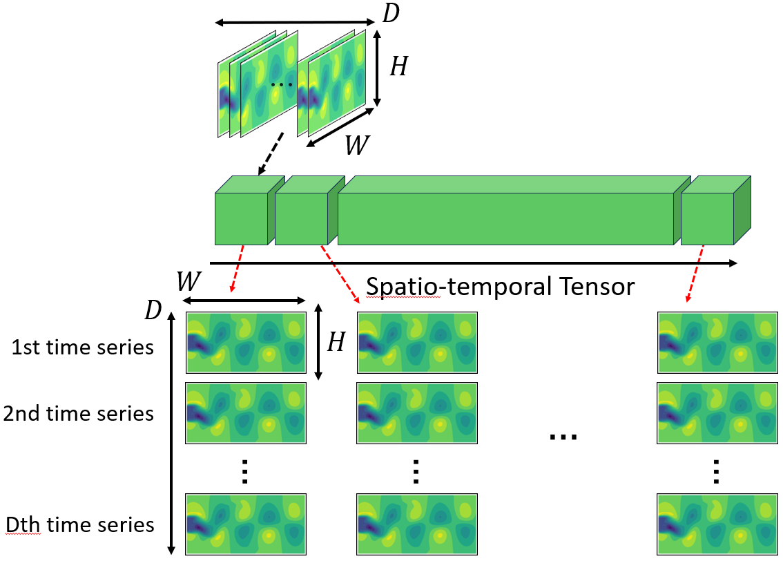
Figure 1: In this work we use datasets represented as spatio-temporal tensors ${\bf Y}$ of shape $(C,W,H,D,T)$. As such, if we focus on just one component of the tensor, then each sample is a tensor itself of shape $(W,H,D)$. To increase the number of available samples we split the dimension $D$ to obtain $D$ matrices of shape $(W,H)$. Repeating this process to all samples in ${\bf Y}$, we obtain $D$ similar time series, composed of matrices. By similar we mean that all series come from the same data generator process.

To start explaining this technique and whithout loss of generality, we will first focus on a single snapshot and a single component of the spatio-temporal tensor ${\bf Y}$, remaining with a three-dimensional snapshot ($W\times H\times D$). Note that we can ”split” the dimension $D$ and obtain $D$ two-dimensional snapshots $(W\times H)$. By repeating the latter to each sample of the tensor ${\bf Y}$ we end up with $D$ time series composed by two-dimensional snapshots instead of a single time series composed by three-dimensional snapshots.

This technique helps to improving the predictions obtain from the ML models, as we are increasing the number of available samples by a factor of $D$. However, this ”splitting” may lead to a loss of information in the dimension $D$ (spanwise) since we no longer consider this dimension as a whole, but independently. Nevertheless, as in this work this technique is only applied to the synthetic dataset, where the flow evolution is almost negligible in the spanwise dimension, we can safely apply this technique without lossing information as we show in Sec. 4.

2.2 Rolling window

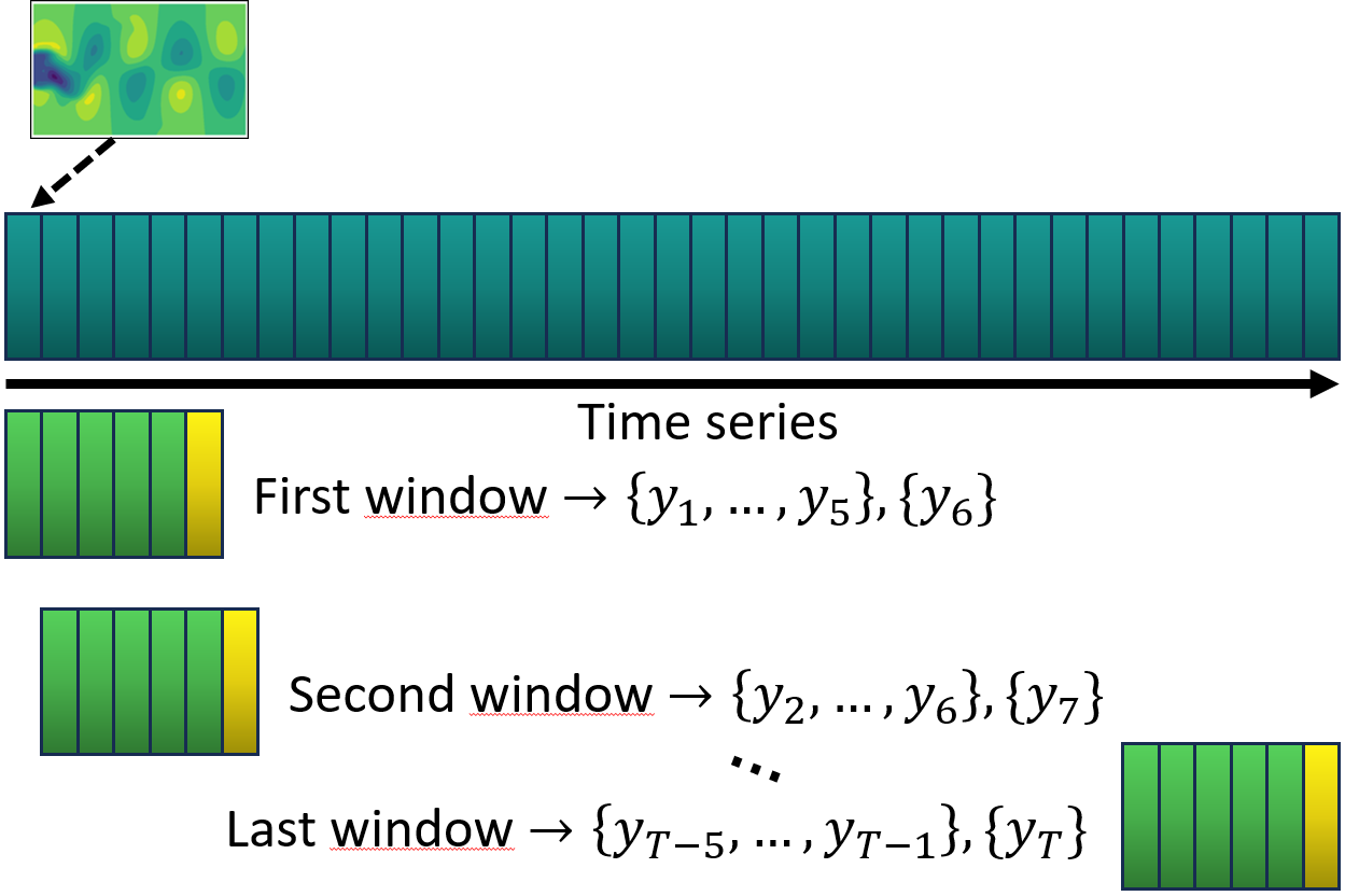
Figure 2: Sliding window method traverses the time series, with a predefined stride, creating windows that contain both the previous samples, which are input to the ML model, and the time-ahead sample that we want to predict. In this representative case we are taking $5$ previous snapshots and asking to predict the next one.

In contrast to the data augmentation technique explained above, which can only be applied to datasets composed by three-dimensional snapshots, and is used to increase the number of time series available for training. The rolling-window technique is a method used to prepare the time series to perform forecasting and can be applied to any dataset. In a time series forecasting problem we need to indicate which samples will be used as input to the ML models (previous sequence) and which ones will be used as target (time-ahead). To do this rolling window traverses the time series, with a predefined stride, creating windows that contain both the previous samples (input to the ML models) and the time-ahead samples, horizon, that we want to predict (target). Applying it to each time series separately, we end up with a set of windows that can be used to train the ML models. Fig. 2 shows a visual depiction of this for a single time series.

It’s important to highlight that depending on the model, we want to predict one or several time-ahead samples. Therefore, the rolling window must be tuned to each model.

3 Methodology

In time series forecasting the aim is to generate a reliable prediction of future events ($y_{t+1},y_{t+2},\dots$), given an available previous information ($y_{1},\dots,y_{t}$). In this work we explore and compare three different methodologies, where two of them are fully based on deep learning (DL) models and a third one is a hybrid model proposed by Abadía-Heredia et al. (2022) that combines singular value decomposition (SVD) Sirovich (1987), Brunton and Kutz (2022) with DL architectures. These models can be splitted in two different methodologies that in literature are identified as: point and probabilistic forecasting Gneiting and Katzfuss (2014). In the former, we want to approximate a deterministic function $f$ as follows,

$$f:[q\times W\times H\times 1]\rightarrow[1\times W\times H\times 1].$$ (2)

In this framework (point forecasting) the function $f$ represents the forecasting process, i.e, we use ML models to approximate a deterministic function that describes the forecasting process $f(\{y_{i}\}_{i=t-q+1}^{t})=y_{t+1}$. To train these models we use the regular mean squared error (MSE).

The other framework (probabilistic forecasting) is similar to the previous one with the difference that instead of approximating a deterministic function, here we want to approximate the probability distribution function $\mathbb{F}_{Y}$ that is behind the forecasting process. The motivation behind this last framework is based on a theoretical proof Bishop (1994), that shows the limits of training dense deep learning models (i.e. neural networks whose architecture is fully composed by dense layers), in regression problems, using the mean squared error against the maximum log likelihood (MLL), where in the latter it is shown that the model is capable to approximate more complex solutions. Actually, the reason to use MSE as loss function in regression problems, comes from a derivation of the maximum log likelihood Goodfellow et al. (2016) (chapter $5.5$).

In this work we use a variational autoencoder (Kingma and Welling, 2022), where the loss function used is the Evidence Lower BOund (ELBO) (Blei et al., 2017), instead of the MLL. However, the ELBO can be understood as a variation of the maximum log likelihood. In the sections below we explain in more detail the proposed models, by starting with the two models inside the point forecasting framework.

3.1 Point forecasting

In this subsection we present the models belonging to the point forecasting methodology, where the aim is to approximate a deterministic function as in (2). Here we use a residual convolutional autoencoder and a hybrid model (SVD + LSTM) as the models that approximate function $f$. The hybrid model has been already previously applied in Abadía-Heredia et al. (2022) and Corrochano et al. (2023), so we recommend to reference to these works to obtained more details about the architecture and applications, as in this section we focus on the description of the residual autoencoder. However, Fig. 3 shows a visual depiction of the methodology that this hybrid model follows.

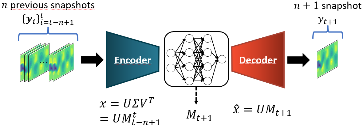
Figure 3: The hybrid methodology can also be represented as an encoder-decoder structure. However, in this case the encoder is just the matrix decomposition ($U,\Sigma,V^{T}$) obtained from SVD. Next we take the temporal information by a matrix multiplication $M_{t-n+1}^{t}=\Sigma*(V_{t-n+1}^{t})^{T}$, and send this matrix to a DL model (hidden layer) which will return the time-ahead sample, i.e., $M_{t+1}$. Finally, the decoder reconstructs the snapshot by multiplying matrices $x_{t+1}=U*M_{t+1}$.

An Autoencoder is formed by an encoder-decoder structure as shown in Fig. 4, and a residual convolutional autoencoder means that both the encoder and decoder are composed by convolutional neural networks (CNN) (Lecun et al., 1998). Tables 5, 6 and 7, in A, show the actual architecture of the model when applied to the experimental dataset. Note in this case the architecture varies depending on the shape of the input snapshots.

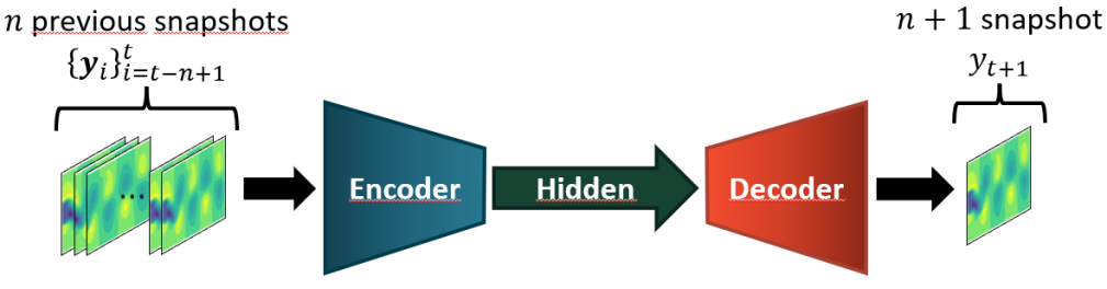
Figure 4: In this case both the encoder and decoder are composed by convolutional neural networks, specifically the encoder is composed by residual convolutional networks and the decoder is composed by transpose convolutional networks. Both of them catch the spatial correlation in data, while the hidden layer is formed by a ConvLSTM network which captures the temporal correlation in data.

The encoder on one side is composed by residual convolutional networks (ResCNN) (He et al., 2016), where the input and output of a CNN are added together. These ResCNNs are mainly defined by the identity and convolutional blocks, which are shown in Fig. 5. Both of them add up the input and output values of the block, with the difference that the identity block neither reduces the size nor modifies the number of channels of the input snapshot, while the convolutional block does it. This architecture allows to speed-up the training and make it more robust. This is based on the fact that asking a CNN to be the identity is more difficult than asking the blocks to be the identity, as in this latter case we are only asking the convolutional kernels to be zero. On the other hand, the decoder is composed by transpose convolutional networks, which perform the inverse operation of a convolutional kernel. It should be highlighted that both the encoder and decoder work on the spatial dimension of the input tensor trying to identify all spatial correlations.

(a)

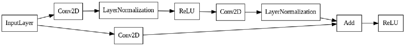
(b)

Figure 5: Visual representation of both types of blocks, identity (top) and convolutional (bottom). Both of them add up the input and output values of the block. However the identity block (top) does not reduce the spatial dimension of the input snapshot while the convolutional block (bottom) does it.

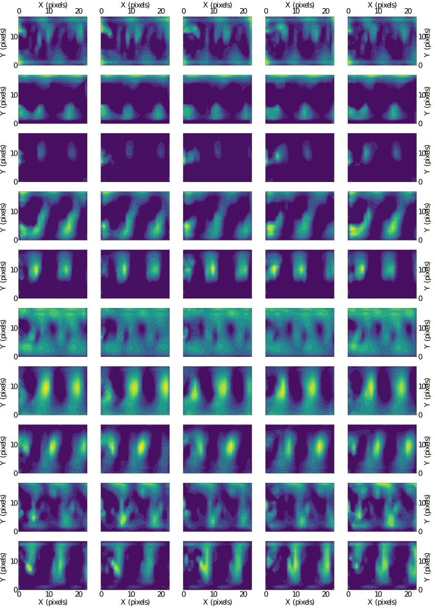
Figure 14: Snapshots of the latent variables obtained from the encoder, in the residual convolutional autoencoder, when the input dataset is the synthetic flow Le Clainche et al. (2018). Note the encoder takes as entries a sequence of $10$ previous snapshots $(10\times 100\times 40\times 3)$ and returns a tensor with size $(10\times 24\times 18\times 64)$. From top to bottom are represented the channels $1,2,3,4,5,10,20,35,55$ and $64$. From left to right is the temporal variation, forward in time, of these channels along $5$ snapshots. Recall from Sec. 3.1 that neither the encoder and decoder modifies the temporal dimension. Unlike the Singular Value Decomposition, which returns the modes sorted by its energy, the encoder does not sort the latent variables. However, something similar to what was done in Muñoz et al. (2023) can be applied to sort them, but this is beyond the scope of this paper. Note that, once the snapshots, regardless of the dataset, are input to the model, their dimensions are no longer the ones coming from the simulation or experiment, but pixels. Therefore, the dimensions of the latent variables shown in this figure are measured in pixels as well.

To capture the temporal correlation in the sequence of previous snapshots $\{y_{i-n+1},y_{i-n+2},\dots,y_{i}\}$, which is the input tensor to the model, we use a hidden layer that is composed by a convolutional LSTM layer (ConvLSTM) (Shi et al., 2015), see Tab. 6 for a more precise information about the architecture. Note from Fig. 4 that this hidden layer is located between the encoder and decoder. Note in this work the encoder and decoder only take information from the spatial dimension of the snapshots ($W\times H$), neither of them modifies the temporal one ($T$). In B, Fig. 14 shows some outputs obtained from the encoder, when the input dataset is the experimental one. Unlike the latent variables obtained from the SVD, these are not hierarchically ordered, based on the information they contain about the flow dynamics. However, the method proposed by Muñoz et al. (2023) can be used to sort them, which was used to order the latent variables of a dense autoencoder.

The reason to locate the ConvLSTM layer between the encoder and decoder is based on the fact that a CNN follows a pyramid scheme, since it represents a single snapshot in multiple smaller ones, where each one contains information about the original snapshot, such as patterns, structures, etc. (Goodfellow et al., 2016). Because of this feature we want to catch the temporal correlations not in the original sequence of snapshots, which are composed by the combination of multiple patterns, structures, etc. But, in their latent spaces, developed by the encoder, where many of these patterns, structures may have been identified and separated Fig. 14. Allowing in this way an easier identification of the temporal correlations.

Note that we decided to use ConvLSTM instead of the regular LSTM (Hochreiter and Schmidhuber, 1997) because the inputs to the model are snapshots and the LSTM layer only accepts vector-formatted entries. This would have forced to flatten the snapshots, returned by the encoder, loosing the spatial information and increasing the number of trainable parameters. On the other way around, ConvLSTM accepts matrix-formatted entries which allows for a more natural flow of the information through the model.

Unlike the variational autoencoder, these two models (hybrid and residual autoencoder) can accept multiple components of the velocity at the same time. While the variational autoencoder can only accept one.

3.2 Probabilistic framework

In contrast to the deterministic framework, here we want to approximate the probability distribution $\mathbb{F}_{Y}$ that is behind the forecasting process of going from a sequence of previous snapshots $\{y_{i-n+1},y_{i-n+2},\dots,y_{i}\}$ to the next one $\{y_{i+1}\}$. With this in mind, we apply the Bayesian point of view of statistical inference (Blei et al., 2017) and develop a variational inference model based on variational autoencoders (Kingma and Welling, 2022). See Fig. 6 for a visual depiction of our proposed model.

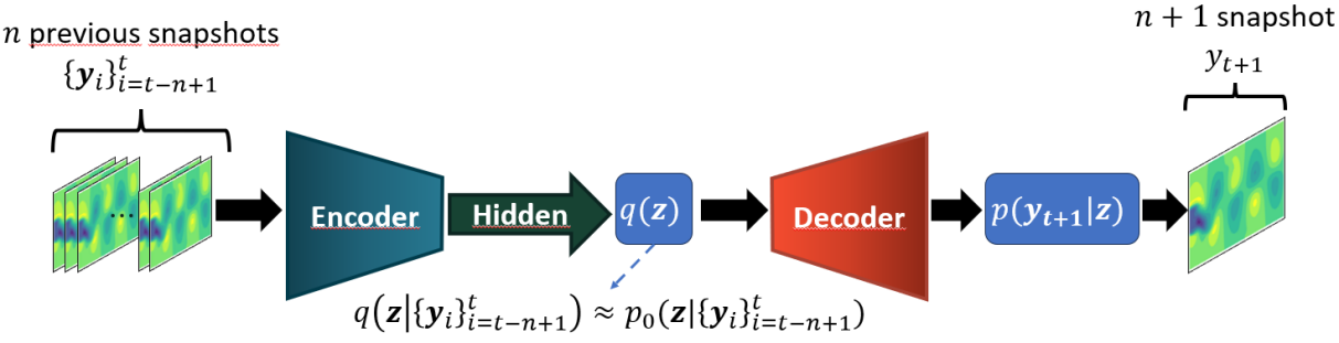
Figure 6: The variational autoencoder proposed in this work. Note that here both the exact and approximate posteriors, $p_{0}(\bm{z}|\cdot)$ and $q(\bm{z}|\cdot)$, respectively, are conditioned on the input sequence of snapshots while we compute the likelihood $p(\bm{y}_{t+1}|\bm{z})$ of the time-ahead snapshot.

Similar to the deterministic framework we have an encoder and decoder that will work on the spatial dimension of the input snapshots. Tabs. 8 and 9 show the specific architecture used when applied to the experimental dataset. Similar to the residual autoencoder, Fig. 4, the architecture varies depending on the size of the input snapshots. There is as well a hidden block that works in the temporal dimension to capture the temporal correlations in the latent space generated by the encoder.

In contrast to both the residual convolutional autoencoder and the hybrid model, in the Variational Autoencoder we approximate the conditional posterior probability function $p_{0}(\bm{z}|\{y_{i}\}_{i=t-n+1}^{t})$ of the latent variables $\bm{z}$ based on the input sequence of snapshots $\{y_{t-n+1},\dots,y_{t}\}$. This conditional posterior $p_{0}(\cdot)$ is parametric, and to choose the optimal parameters we use the information coming from the encoder and hidden blocks. Next, we also approximate the likelihood $p(y_{t+1}|\bm{z})$ of the time-ahead snapshot $\{y_{t+1}\}$ based on the latent variables $\bm{z}$.

Note from Fig. 6 that the decoder input comes from the posterior distribution $p_{0}(\bm{z}|\{y_{i}\}_{i=t-n+1}^{t})$. Therefore, we need to generate a sample from this posterior and use it as input to the decoder. The same is done with the likelihood $p(y_{t+1}|\bm{z})$ to obtain the time-ahead predicted snapshot.

The original variational autoencoder presented in (Kingma and Welling, 2022) was applied to approximate the probability distribution function behind a set of images. After training, what can be done is to randomly generate a sample from the approximated posterior, pass that sample into the decoder and finally generate a new image from the likelihood. In this way the variational autoencoder can be understood as a randomly image generator. In that paper the loss function used is the Evidence Lower Bound (ELBO), which is described as follows:

$$\hbox{ELBO}=\mathbb{E}[\hbox{log}\ p(\bm{x}|\bm{z})]-\hbox{KL}[q(\bm{z}|\bm{x})||p_{0}(\bm{z}|\bm{x})].$$ (3)

Where $\bm{x}$ is the input image, $p_{0}(\bm{z}|\bm{x})$ is the exact posterior distribution of the latent variables $\bm{z}$, $q(\bm{z}|\bm{x})$ is the approximate posterior and $p(\bm{x}|\bm{z})$ is the likelihood of the image $\bm{x}$ given the latent variables $\bm{z}$. Note that in (3) the ELBO is only evaluated in a single image $\bm{x}$. In this work we explore a modification of this loss function, where we condition both the exact and approximate posterior on the input sequence of snapshots $\{y_{i}\}_{i=t-n+1}^{t}$ instead of a single image $\bm{x}$. Also, we now want to approximate the likelihood of the time-ahead snapshot $p(y_{t+1}|\bm{z})$. Therefore the loss function that we use to train the VAE is as follows,

$$\hbox{ELBOf}=\mathbb{E}[\hbox{log}\ p(y_{t+1}|\bm{z})]-\hbox{KL}[q(\bm{z}|\{y_{i}\}_{i=t-n+1}^{t})||p_{0}(\bm{z}|\{y_{i}\}_{i=t-n+1}^{t})].$$ (4)

This loss function allows us to approximate the likelihood of the time-ahead snapshot based on the latent variables $\bm{z}$ that are obtained from the previous sequence of snapshots $\{y_{i}\}_{i=t-n+1}^{t}$.

4 Results and discussion

In the following sections we present the predictions obtained from the three models when they are applied to the synthetic dataset (Sec. 4.1), and the experimental dataset (Sec. 4.2). We show in Tab. 1 the time required to either train each model and to generate the time-ahead predictions. As was stated at the beginning of Sec. 2 the datasets correspond to the steady state of each flow.

Dataset	Model	Training length (epochs)	Training time (min.)	Prediction time (sec.)
Synthetic
	Hybrid	420	$2.622$	$1.546$
	Residual AE	25	$82.837$	$160.633$
	VAE	20	$43.330$	$45.770$
Experimental
	Hybrid	$420$	$30.418$	$1.683$
	Residual AE	$120$	$329.665$	$29.094$
	VAE	$14$	$13.966$	$14.746$

Table 1: Training length measured in number of epochs, training time measured in minutes and generation of time-ahead snapshots measured in seconds for each one of the three ML models (hybrid, residual autoencoder and variational autoencoder) and each dataset (synthetic and experimental), respectively. Note the synthetic flow is composed by three-dimensional snapshots, and the experimental flow is composed by two-dimensional snapshots.

Note the models presented in this work are autoregressive, i.e., these models use the time-ahead prediction ($y_{t+1}$) from previous time steps ($\{y_{t-n+1},\dots,y_{t}\}$) as a new input (i.e., $\{y_{t-n+2},\dots,y_{t},y_{t+1}\}$) to generate a new prediction ($y_{t+2}$), and so on. In both datasets we ask the models to generate $200$ time-ahead snapshots, three-dimensional in the synthetic dataset and two-dimensional in the experimental.

Independently of the datasets, to train the models, we used the optimization method known as Adam Kingma and Ba (2017) with the default values for the parameters $\beta_{1}=0.9$, $\beta_{2}=0.999$ and $\epsilon=10^{-8}$ (see details in Kingma and Ba (2017)). However, the learning rate $\alpha$ differs between models, see Tab. 2. Also, both the length of the input sequence and the number of time-ahead predictions generated by the models differ between the models and datasets, see Tab. 2. The number of training and testing samples for each dataset, which are independently of the model, is shown in Tab. 3.

Model	Learning rate ($\alpha$)	Length input sequence	$\#$ predictions generated
Hybrid	$10^{-3}$	$10$	$6$
Residual AE	$5\times 10^{-4}$	$10$ (synth.) / $5$ (exp.)	$1$
VAE	$5\times 10^{-5}$	$10$ (synth.) / $5$ (exp.)	$1$

Table 2: Number of snapshots used for both training and testing the ML models. Note the length of the input sequence of snapshots varies depending on the dataset for the residual autoencoder and the variational autoencoder, but not for the hybrid model.

Dataset	Snapshot dimension	Training	Testing	Total
Synthetic	3D	$199$	$300$	499
Experimental	2D	2800	1200	4000

Table 3: Number of snapshots used for both training and testing the ML models. Note the synthetic flow is composed by three-dimensional snapshots, while the experimental flow is composed by two-dimensional snapshots.

To quantitatively measure how close the predictions are to the ground truth we use two metrics. One is the relative root mean squared error (RRMSE), which is defined as in equation (5).

$$\hbox{RRMSE}=\sqrt{\frac{\sum_{k=1}^{K}||y_{k}-\tilde{y}_{k}||^{2}}{\sum_{k=1}^{K}||y_{k}||^{2}}}.$$ (5)

Where $y_{k}$ is the $k$-th ground truth snapshot and $\tilde{y}_{k}$ is the $k$-th prediction obtained from the ML model. As we are comparing snapshots, we also use the structural similarity index measure (SSIM) Wang et al. (2004), Wang and Bovik (2009) to measure the degree of similarity between them, based on their structural information. Both metrics return measures belonging to the interval $[0,1]$, but while for the RRMSE $0$ is the best and $1$ the worst, for the SSIM $1$ is the best and $0$ the worst.

In the next section we start by showing and discussing the results obtained from the three models when they are applied to the synthetic dataset, which represents a three-dimensional wake of a circular cylinder obtained by a numerical simulation Le Clainche et al. (2018).

4.1 Synthetic flow

This dataset represents a three-dimensional wake of a circular cylinder, where the first $100$ time steps correspond to the transitory state of the flow, as is shown in Fig. 7. It is well know that in this state the flow statistics are constantly varying, thus these first time steps are not taken into account for training and testing the models. Fig. 7 shows how time steps from $100$ to $299$ are used to train the models, while the rest ($300$ to $599$) are used to testing. From here we conclude that $50\%$ of the available samples are used for training.

Since this dataset is composed by three-dimensional snapshots, we are able to use the data augmentation technique defined in Sec. 2, which allows us to go from $199$ samples to $199*D=199*64=12736$ samples. Note, this data augmentation is only used for the residual and variational autoencoders, because the hybrid model does not receive snapshots as input, but vectors representing the POD coefficients from SVD Abadía-Heredia et al. (2022).

Note in Fig. 7 (a) how the flow statistics in the streamwise velocity slightly changes around the time instant $350$. This is an interesting case, because that variation in the statistics is not observed in the training samples, which allow us to see how the models will behave in such a scenario.

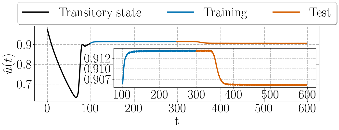
(a)

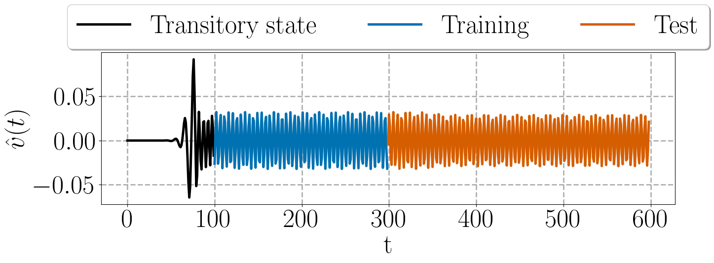
(b)

Figure 7: Mean flow velocity $\hat{u}(t)$, $\hat{v}(t)$ evolution in the synthetic dataset. In both figures (a) and (b) can be observed that the transitory state happens from instant $0$ to $99$. In this dataset we use as training the time instants from $100$ to $299$, while the rest (from $300$ to $599$) is left to testing.

Once the models have been trained, we iteratively predict $200$ snapshots ahead in time ([$300$ - $499$]), and compare the statistics of the predicted snapshots with the ground truth snapshots obtained from the numerical simulation. In Fig. 8 we can observe this comparison where figures (a), (c) and (e) shows the predictions obtained in the streamwise velocity from the hybrid, residual autoencoder and variational autoencoder, respectively. Figure (b), (d) and (f) shows the same but for the wall-normal velocity. Note how in the streamwise velocity the hybrid and VAE predictions mean are very close to the ground truth, at least until the mean decay where non of the models are capable to predict this variation in the mean. This is because such a variation is not observed in the training samples and these models are not physics informed. However, as in the wall-normal component there is not a variation in the mean, the predictions mean of the models are very close to the ground truth mean. Nevertheless, at least in the mean, predictions from the hybrid and VAE models looks more accurate than the ones generated by the Residual autoencoder.

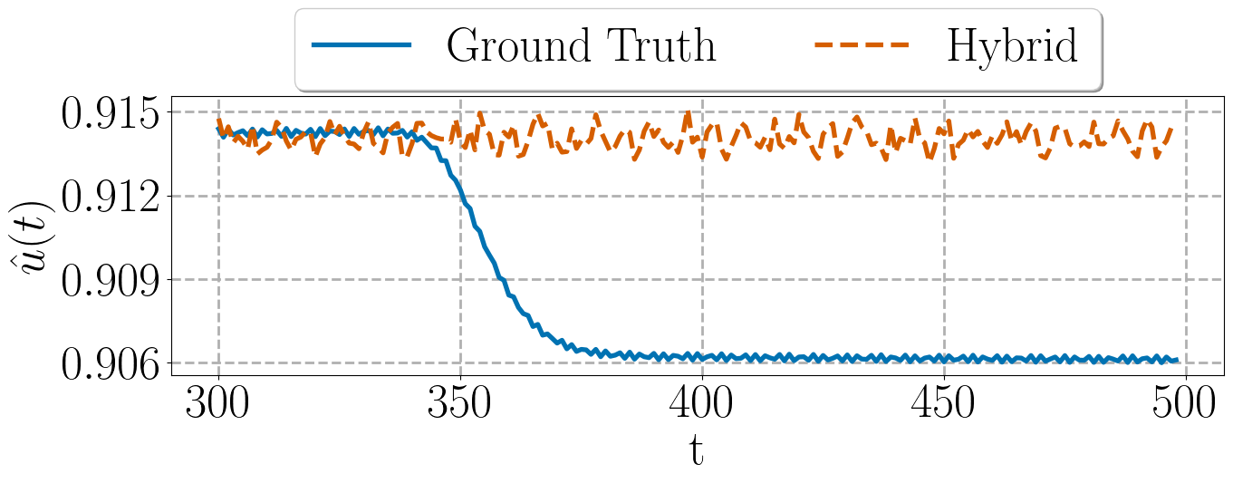
(a)

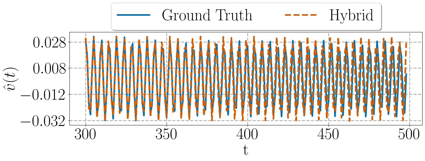
(b)

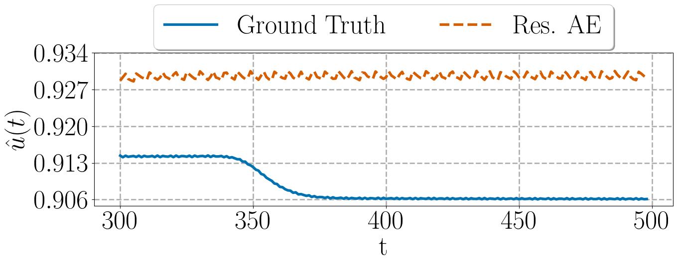
(c)

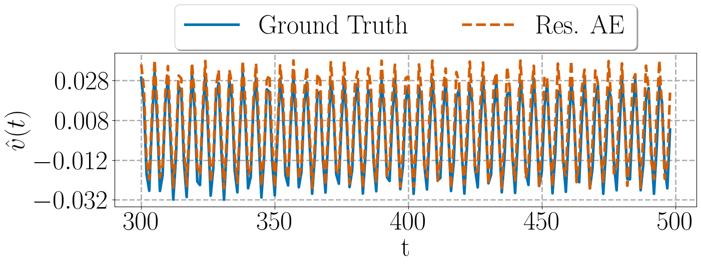
(d)

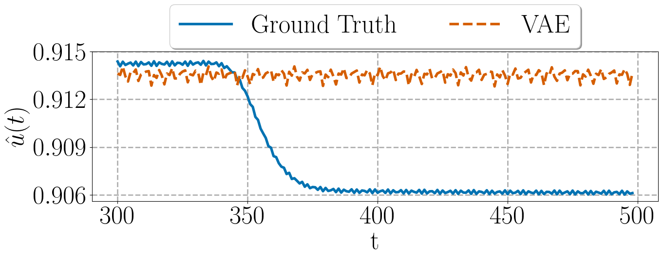
(e)

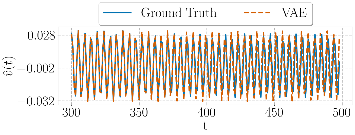
(f)

Figure 8: Mean flow velocity at each time instant. Figures (a), (c) and (e) compare the ground truth mean of the streamwise velocity $\hat{u}(t)$ against the prediction generated by the hybrid, residual autoencoder and variational autoencoder models, respectively. Figures (b), (d) and (f) do the same for the wall-normal velocity component $\hat{v}(t)$. In all figures the ground truth is represented by a solid line and the prediction by a dashed line.

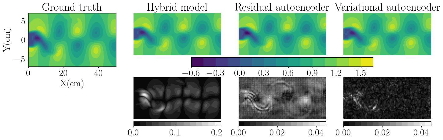
(a) Ground truth snapshot and predictions at time instant $300$.

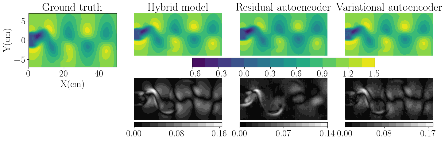
(b) Ground truth snapshot and predictions at time instant $340$.

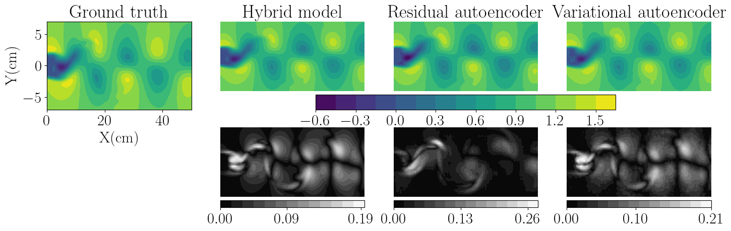
(c) Ground truth snapshot and predictions at time instant $360$.

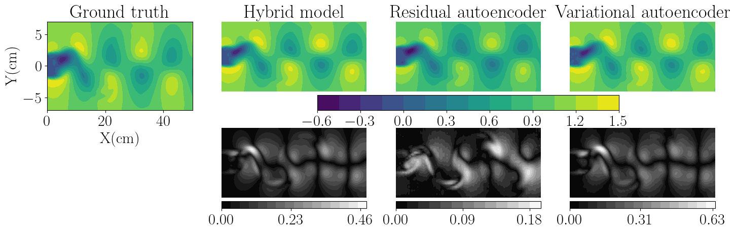
(d) Ground truth snapshot and predictions at time instant $425$.

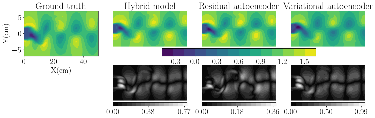
(e) Ground truth snapshot and predictions at time instant $499$.

Figure 15: Snapshots at some representative time instants showing the ground truth streamwise velocity component and the predictions obtained from the different models. The time instants chosen are $300$, $340$, $360$, $425$ and $499$. Note for this dataset the dimensions of the snapshots are in centimeters (cm).

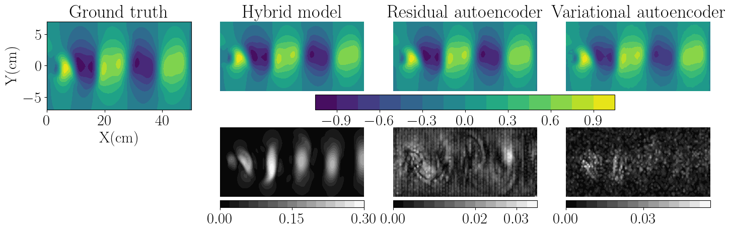
(a) Ground truth snapshot and predictions at time instant $300$.

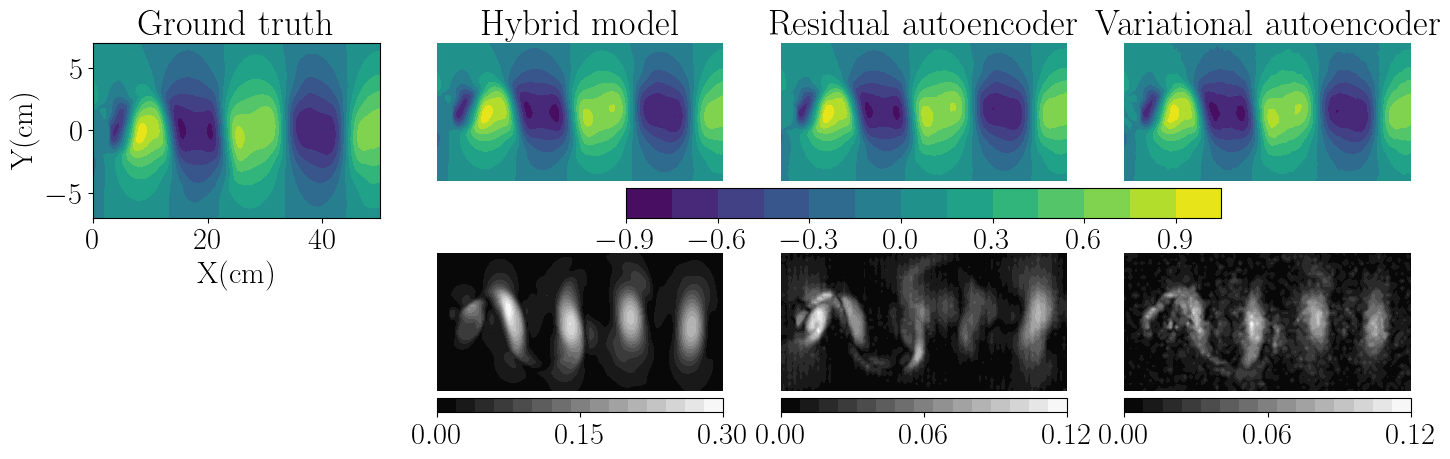
(b) Ground truth snapshot and predictions at time instant $340$.

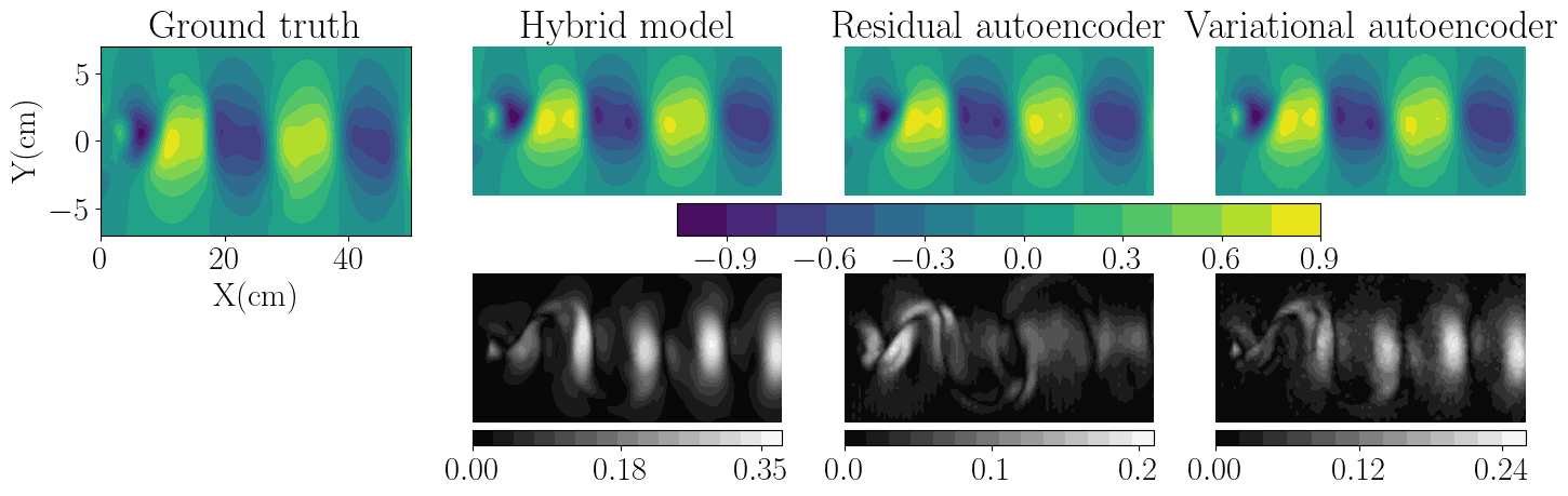
(c) Ground truth snapshot and predictions at time instant $360$.

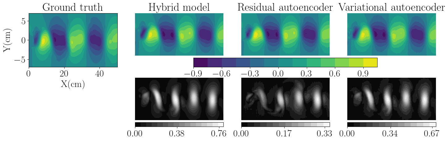
(d) Ground truth snapshot and predictions at time instant $425$.

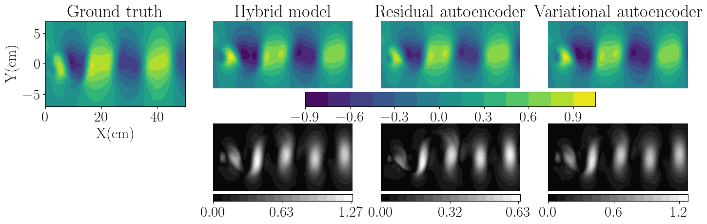
(e) Ground truth snapshot and predictions at time instant $499$.

Figure 16: Snapshots at some representative time instants showing the ground truth wall-normal velocity component and the predictions obtained from the different models. The time instants chosen are $300$, $340$, $360$, $425$ and $499$. Note for this dataset the dimensions of the snapshots are in centimeters (cm).

To check the latter we measure how similar are these predictions to the ground truth using both the RRMSE defined in equation 5 and the SSIM, which measures how similar are two figures based on their structural information. Fig. 9 shows the measures obtained by these two metrics in the synthetic dataset. Note how, in contrast to what is shown in Fig. 8, the most accurate predictions are obtained from the residual autoencoder. As the predictions are generated iteratively, it is intuitive to think that stored error will make predictions further out in time worse. However, the residual autoencoder is found to be more stable over time. The same can be qualitatively observed in Figs. 15 and 16 where some representative snapshots are plotted comparing the ground truth and predictions obtained from the three models. We believe this can be explained by looking at Figs. 15 and 16 where in time steps $425$ and $499$ it can seen how the predictions of the hybrid model and variational autoencoder are shifted. While in the residual autoencoder, although they are also shifted, they are not so shifted.

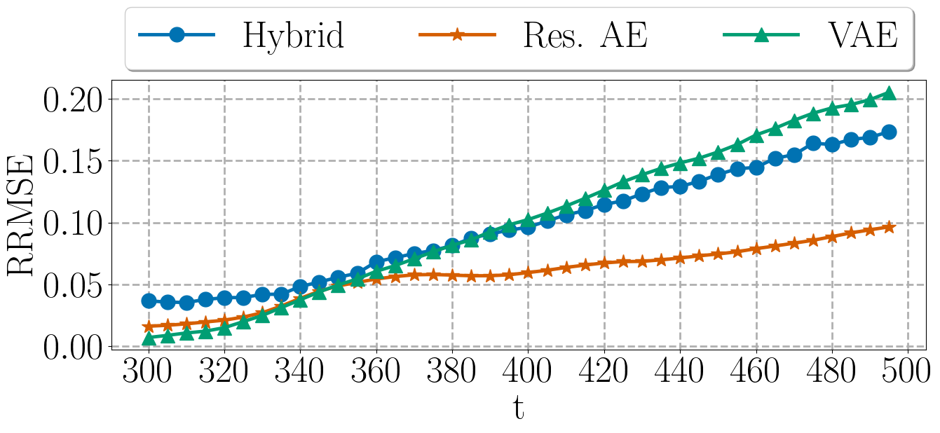
(a)

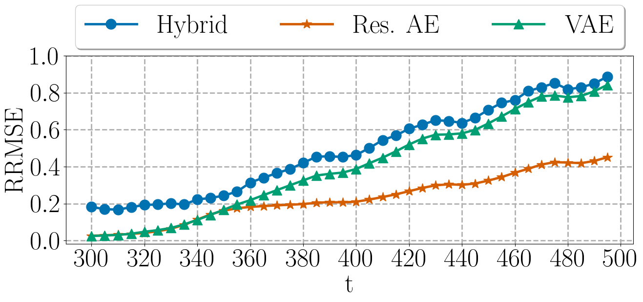
(b)

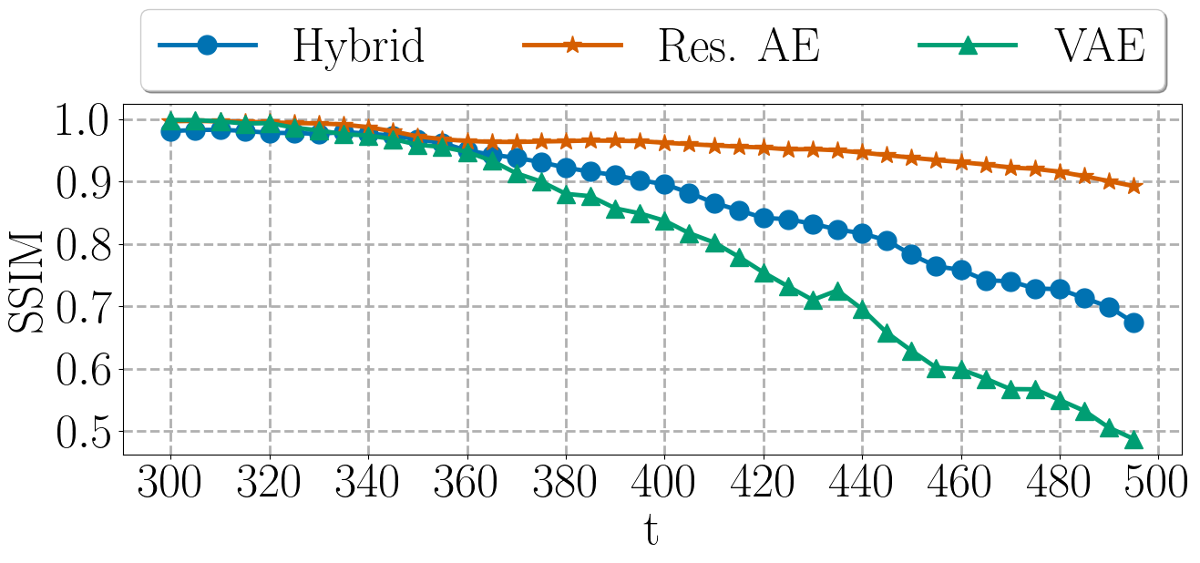
(c)

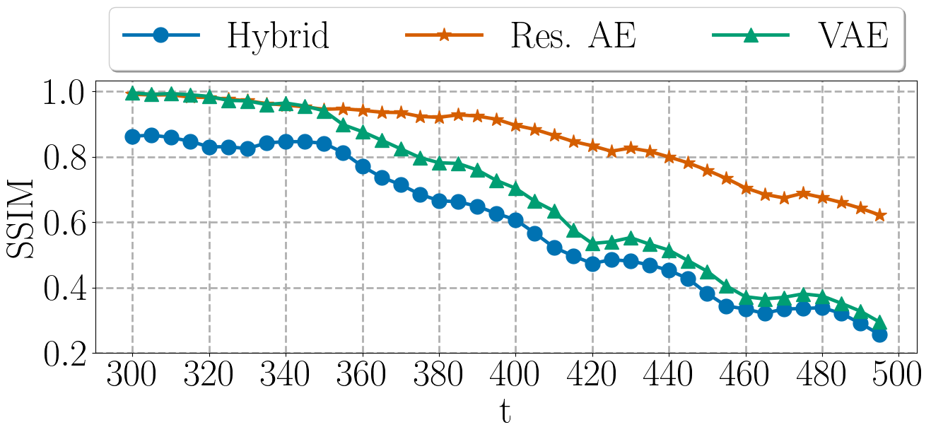
(d)

Figure 9: To measure how accurate are the predictions we use the RRMSE and SSIM, while the RRMSE is a variation of the classical mean squared error, the SSIM measures how similar are two figures based on their structural information. Mesures from RRMSE are shown in (a) and (b) for the streamwise and wall-normal velocity, respectively. While, measures from SSIM are shown in (c) and (d) for the streamwise and wall-normal velocity, respectively. For the synthetic dataset, 200 snapshots were generated iteratively.

From here we can assume that the model that best captures the flow dynamics is the residual autoencoder, followed by the hybrid model. Being the VAE who returned worse predictions. We believe this is due to the ELBO loss function defined in equation (4). Where it is intended to approximate a probability distribution function. This loss function is more complex than MSE, which is the one used to train both the hybrid and residual autoencoder. This may cause the model to require more training data than the other two.

In the following section we show and discuss the results obtained from the three models when they are applied to the experimental dataset, which as well represents a flow past a circular cylinder, with the difference that this flow is two-dimensional and the data was obtained by measurements of an experimental setup Mendez et al. (2020).

4.2 Experimental flow

This dataset corresponds to an experimental flow representing a three-dimensional wake of a circular cylinder at high Reynolds number ($\hbox{Re}=[2600-4000]$). Specifically we take the data corresponding to the streamwise velocity in its first steady state before the transitory phase, see Fig. $1$ in Mendez et al. (2020). The dataset is composed by a total of $4000$ two-dimensional snapshots, from which the first $2800$ are taken to training and the rest is left to testing. In Fig. 10 is shown the mean of the streamwise velocity at each sample, and a visual depiction of the training-test data division. Note that since this dataset is composed by two-dimensional snapshots, we cannot use the data augmentation technique defined in Sec. 2 to increase the available number of training samples.

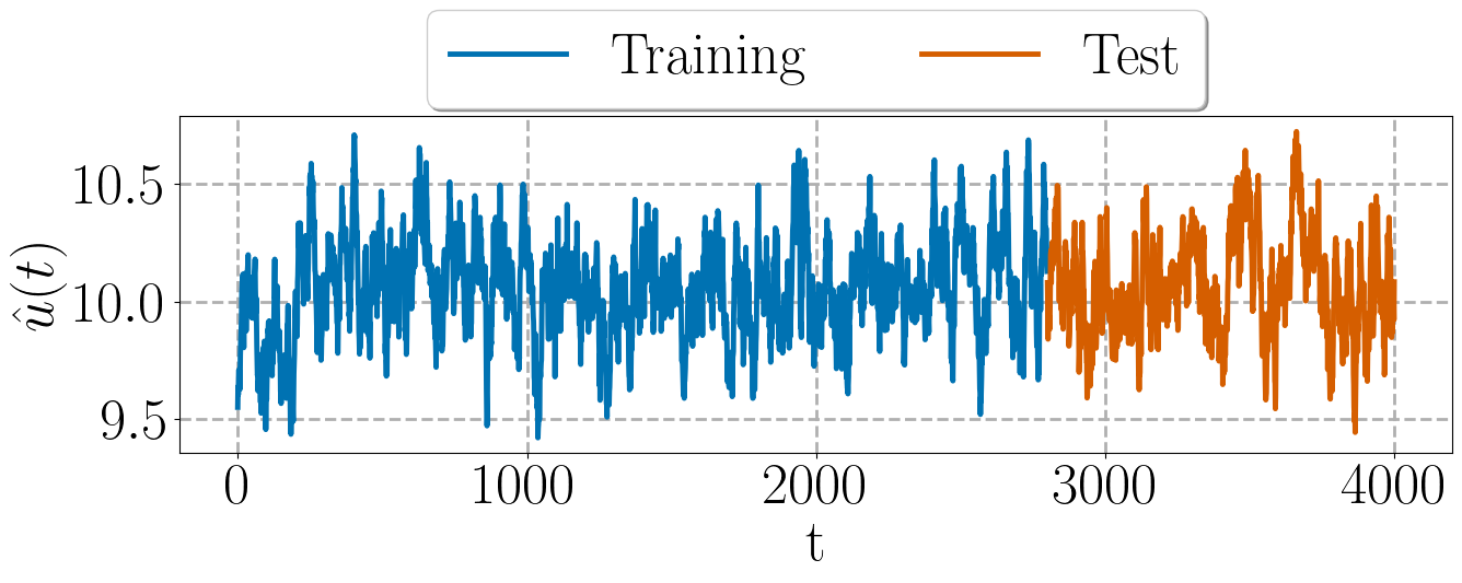
Figure 10: Mean flow streamwise velocity $\hat{u}(t)$ evolution in the experimental dataset. Here we use the first $2800$ samples to training, while the rest is left to testing.

Looking at Fig. 10, it can be seen that this flow is much more complex than the synthetic one, Fig. 7. This is due to the high Reynolds numbers at which the flow was investigated. After several trials we conclude that for this flow the best option is to simplify the dynamics by reconstructing it through singular value decomposition (SVD), i.e., for the reconstruction we only consider the most energetic modes that contains the principal dynamics. In this work we keep the first $100$ modes to reconstruct the flow. Tab. 4 shows the difference between the original flow coming from experimental measurements and the reconstruction performed using SVD, keeping the first $100$ modes.

This simplified dataset is the one used to train both the residual and variational autoencoders, as the hybrid is already applying SVD we train this model with the original dataset. We only apply SVD to the first $2800$ samples that we use for training the models. The aim of this is to train the models in a simplified dataset, a similar procedure was carried out in Mata et al. (2023).

Original	SVD reconstruction

Table 4: Comparison of the original flow from experimental measurements and the reconstruction using SVD, keeping the 100 most energetic modes.

Once the models are trained, we iteratively predict $200$ snapshots ahead in time ([$2801$ - $3000$]), and compare the statistics of the predicted snapshots with the ground truth snapshots obtained from measurements in the experiment. In Fig. 11 we can observe this comparison where figures (a), (b) and (c) shows the predictions obtained in the streamwise velocity from the hybrid, residual autoencoder and variational autoencoder (VAE) models, respectively. Note how predictions from the hybrid model are the only ones that follow the trend of the ground truth, in contrast to what we obtained in the synthetic flow, where both the residual autoencoder and the hybrid model returned good predictions. Looking at the mean, we can guess that predictions from the hybrid model are by far more accurate than the ones generated by the residual autoencoder and VAE.

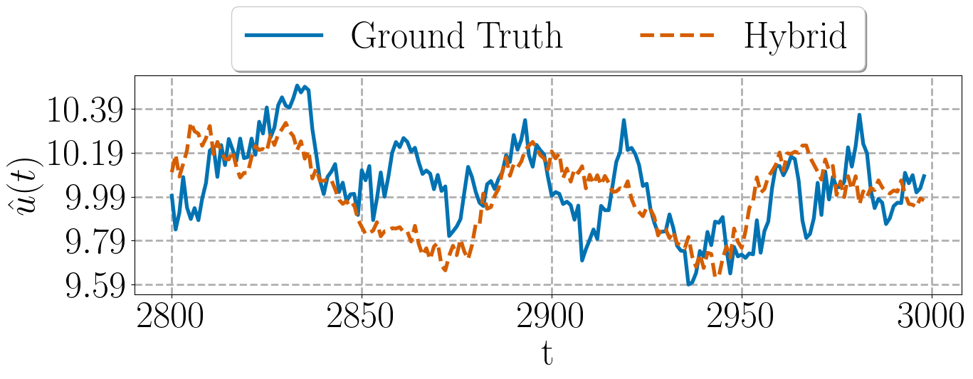
(a)

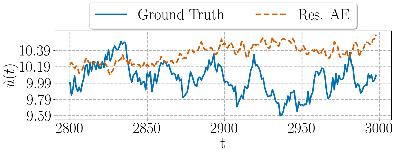
(b)

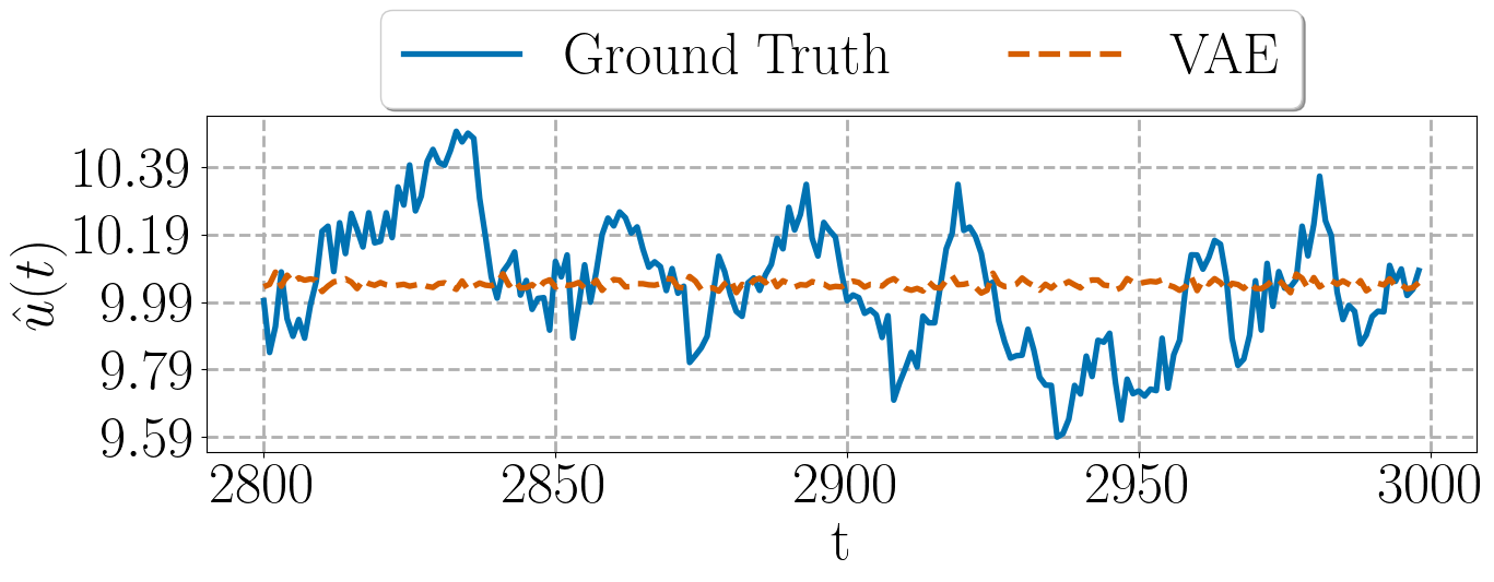
(c)

Figure 11: Mean flow velocity at each time instant in the experimental flow. Where figures (a), (b) and (c) compare the ground truth mean of the streamwise velocity $\hat{u}(t)$ against the prediction generated by the hybrid, residual autoencoder and variational autoencoder, respectively. In all figures the ground truth is represented by a solid line and the prediction by a dashed line.

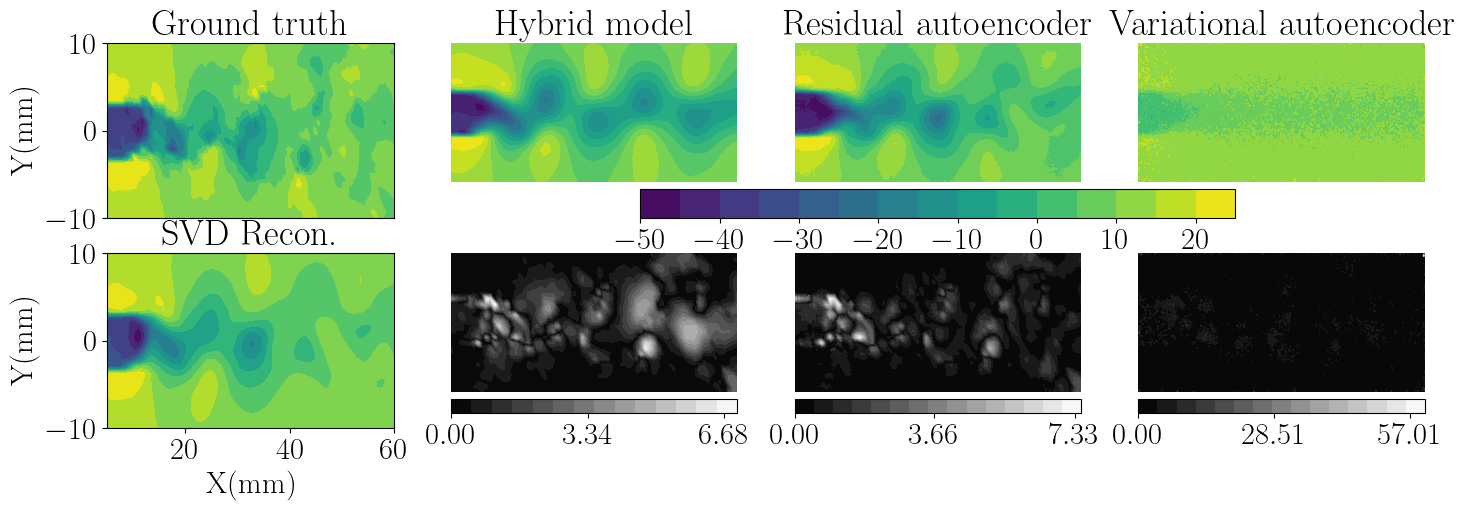
(a) Ground truth snapshot and predictions at time instant $300$.

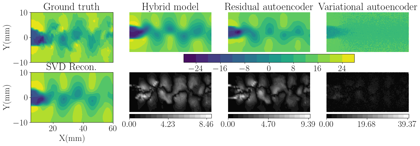
(b) Ground truth snapshot and predictions at time instant $340$.

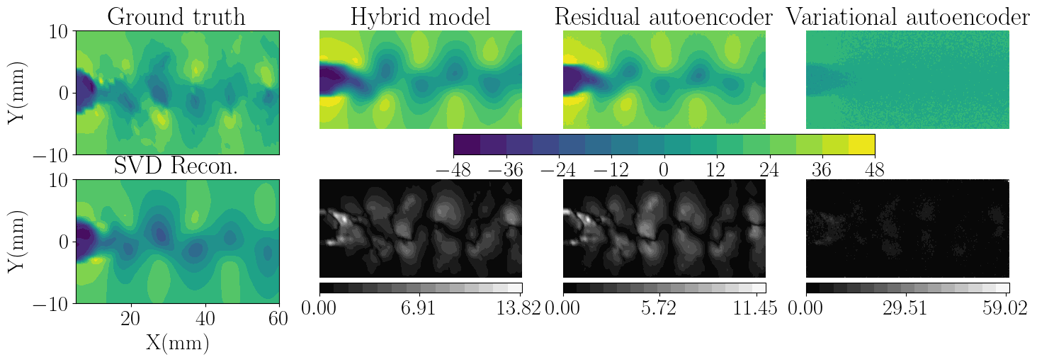
(c) Ground truth snapshot and predictions at time instant $360$.

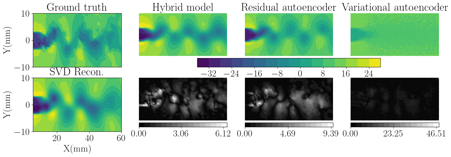
(d) Ground truth snapshot and predictions at time instant $425$.

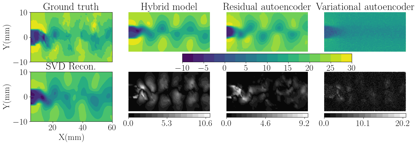
(e) Ground truth snapshot and predictions at time instant $499$.

Figure 17: Snapshots at some representative time instants showing the ground truth streamwise velocity component and the predictions obtained from the different models. The time instants chosen are $2800$, $2850$, $2860$, $2950$ and $3000$. Note for this dataset the dimensions of the snapshots are in millimeters (mm).

Similar to the synthetic flow, we measure how similar are these predictions to the ground truth using both the RRMSE defined in equation 5 and the SSIM. Fig. 12 shows the measurements obtained by these two metrics in the experimental flow. Note how the assumption we made when looking at the mean is now confirmed by the measurements returned by the RRMSE and SSIM. Where the best ones correspond to the hybrid model. Also, note the importance of using the SSIM metric apart from the RRMSE, because when looking at Fig. 12 (a) one can think that all models are generating predictions with similar accuracy, but when looking at figure (b) we can clearly see that predictions from VAE are not even close to ground truth data. This is because SSIM uses structural information to measure the similarity between two snapshots. This large difference, in accuracy, between the predictions can be also observed in Fig. 17.

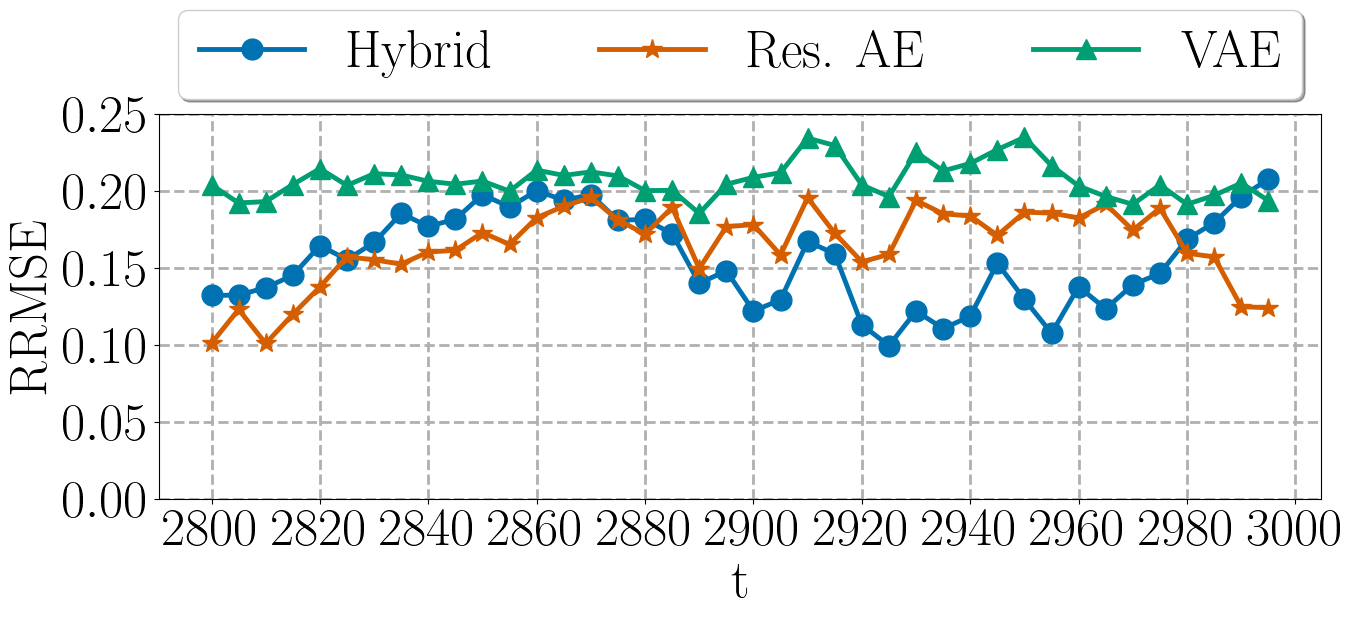
(a)

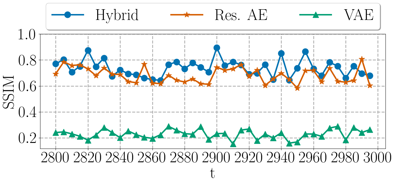
(b)

Figure 12: To measure how accurate are the predictions in the streamwise velocity, we use the RRMSE and SSIM, while the RRMSE is a variation of the classical mean squared error, the SSIM measures how similar are two figures based on their structural information. Mesures from RRMSE are shown in (a), and measures from SSIM are shown in (b). For the experimental flow, $200$ time-ahead snapshots were generated iteratively ([$2801$ - $3000$]).

Since the experimental flow is turbulent, trying to predict the exact state-space, velocity flow field, is almost an impossible task due to all the small scales and randomness occurring inside the dynamics. However, predicting the flow statistics is a much simpler task. Thus, in Fig. 13 we compare the velocity magnitude histograms of the snapshots we want to predict, and the predictions obtained from the three models. Note, the predictions from the hybrid model follow a distribution closer to the ground truth data than the other two models, which is in tune with the results shown in Figs. 12 and 11.

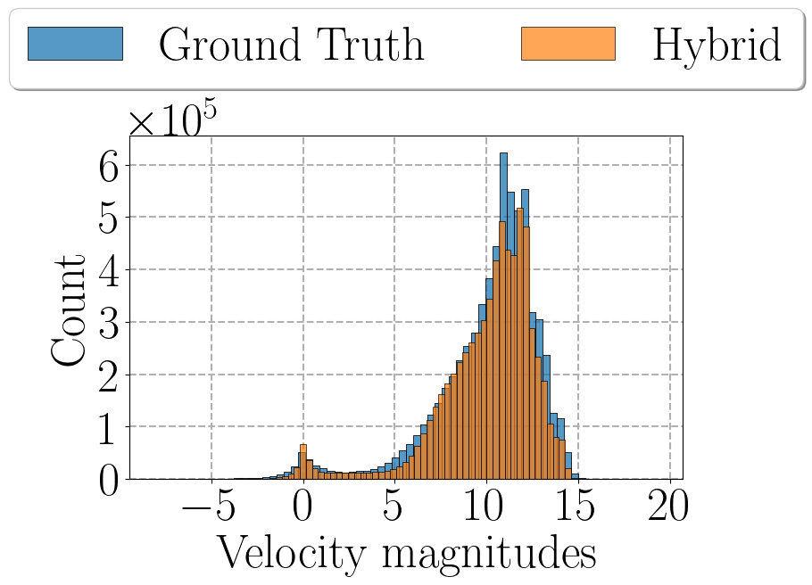
(a)

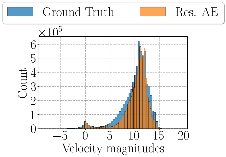
(b)

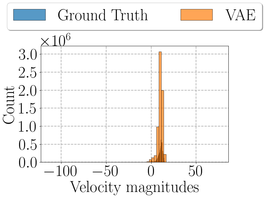
(c)

Figure 13: Comparison of the velocity histograms from the snapshots that we want to predict in the experimental dataset, and predictions obtained from (a) the hybrid model, (b) the residual autoencoder and (c) the variational autoencoder. Note, predictions from the hybrid model follow a distribution closer to the ground truth data than the other two models.

4.3 General discussion

From these two test cases we have observed how the models behave and how stable they are in iteratively generating predictions about the flow dynamics. The low performance of the VAE model could be explain by the complexity of the loss function ELBO, which is designed to approximate a probability distribution function. However, as was stated in Sec. 3 the motivation to this model comes from the flexibility a feedforward network gains to approximate more complex solutions, when it is train with the maximum log likelihood (MLL) instead of the mean squared error (MSE) Bishop (1994). Although the theoretical proof focuses only on regression problems and feedforward networks, similar proposals have been made in the field of probabilistic forecasting Gneiting and Katzfuss (2014), like temporal diffusion models Lin et al. (2023) or copulas methods for forecasting multivariate time series Patton (2013); Smith (2023). Therefore, we do not rule out that models based on probabilistic forecasting can predict flow dynamics.

Regarding the other two models, both of them use the MSE as loss function. However, while the hybrid model combines singular value decomposition (SVD) with an LSTM architecture, the residual autoencoder is fully based on deep learning, it is composed by convolutional networks and transpose convolutional networks. Note, on the one hand, the hybrid model does not predict snapshots by itself, but temporal modes, which are then used to reconstruct the snapshots. On the other hand, the residual autoencoder predicts the snapshots, without the need for any post-processing to reconstruct them.

The main advantage of the hybrid model is the huge reduction in dimension, since we replace the two-dimensional snapshots as input by a simple vector whose size depends on the number of modes retained. However, the SVD decomposes a dataset in three differente matrices ($U$, $S$, $V^{T}$). Where we use $S$ and $V^{T}$ to perform the forecast, and keep $U$ as is, which is then use to reconstruct the snapshots. Therefore, we are assuming that this matrix $U$ does not vary, which may not actually be true, as it may have a slight variation as we go forward in time. In Fig. 9 we observed how the hybrid model generates worse predictions than the residual autoencoder, we believe it is due to this variation in the $U$ matrix that we are not accounting for. Nevertheless, in Fig. 12 and specially in Fig. 11 we can clearly identify that the best predictions are by far returned by the hybrid model. In this sense, even if we continue to believe that the variation in $U$ matrix is leading to errors, they are not too big, allowing the hybrid model to catch the main dynamics.

One big difference between the hybrid model and the residual autoencoder, is that the latter have to modify its architecture depending on the size (i.e., resolution) of the incoming snapshots. This could be addressed by using spatial pyramid pooling He et al. (2014), which resize every input snapshots to a fixed size, in addition this technique drives the identification of multiple scales inside the snapshot. Although, this technique looks like an alternative its implementation will add complexity to the model. For this reason we believe the hybrid model is the one with best properties, as it reduces the dimension of the incoming snapshots to vectors, which contains the main dynamics of the flow, simplifying both the architecture required and the training. This also makes it more intuitive to apply multivariate forecasting methods and theory than using two-dimensional snapshots. But more importantly, the hybrid model can be applied to different datasets without much modification to the predictive model.

5 Conclusions

In this work we have studied the performance of three autoregressive forecasting models, each following a different methodology. One hybrid model that combines singular value decomposition with a long-short term memory architecture and two fully-based deep learning models: a residual autoencoder and a variational autoencoder. We have applied these models to fluid dynamics datasets, which are characterize of being multidimensional and nonlinear. The high dimensionality of these datasets lead us to develop methods that make use of the latent dimension, i.e., models that decompose the high dimensional dataset to a reduced order representation in a bijective way. We did this following a stochastic methodology, using autoencoders, and a deterministic methodology, using singular value decomposition. Then we predict the future evolution of this reduced order representation to finally recover the original dimensionality, thanks to the bijective property. We have tested these models in both a numerical and a experimental dataset, where the latter is characterized by being a turbulent flow. We have observed that both the variational and the residual autoencoders were able to achieve accurate predictions in the numerical dataset, while in the experimental one, only the residual autoencoder was able to generate predictions close to the ground truth data. However, the hybrid model was not only able to achieve similar results, in terms of accuracy, on the numerical dataset, but outperformed the other two on the experimental dataset, demonstrating the generalization capabilities of these hybrid-type models. Also, its ability to reduce the dimension of the incoming snapshots, applying singular value decomposition, allows to either reduce the architecture complexity of the forecasting model and the training data required. We believe that this work has demonstrated the potential of machine learning-based models, specifically when combined with modal decomposition techniques, to predict the evolution of flow dynamics. Although further research is still needed, especially in the area of probabilistic forecasting, this kind of tools have a wide variety of applications in both industry and academia.

Appendix A

# Layer	Layer details	Kernel size	Stride	Padding	Activation	# Params.	Dimension
$0$	Input	-	-	-	-	-	$10\times 100\times 40\times 2$
$1$	Conv 2D	$3\times 3$	$2\times 1$	Valid	ReLU	$448$	$10\times 49\times 38\times 16$
$1$	LayerNorm.	-	-	-	-	$32$	$10\times 49\times 38\times 16$
$2$	Conv 2D	$3\times 3$	$1\times 1$	Valid	ReLU	$4640$	$10\times 47\times 36\times 32$
$2$	LayerNorm.	-	-	-	-	$64$	$10\times 47\times 36\times 32$
$3$	Identity B.	$3\times 3$	$1\times 1$	Same	ReLU	$18560$	$10\times 47\times 36\times 32$
$4$	Identity B.	$3\times 3$	$1\times 1$	Same	ReLU	$18560$	$10\times 47\times 36\times 32$
$5$	Identity B.	$3\times 3$	$1\times 1$	Same	ReLU	$18560$	$10\times 47\times 36\times 32$
$6$	Conv B.	$3\times 3$	$2\times 2$	Valid	ReLU	$57600$	$10\times 24\times 18\times 64$
$7$	Identity B.	$3\times 3$	$1\times 1$	Same	ReLU	$73984$	$10\times 24\times 18\times 64$
$8$	Identity B.	$3\times 3$	$1\times 1$	Same	ReLU	$73984$	$10\times 24\times 18\times 64$
$9$	Identity B.	$3\times 3$	$1\times 1$	Same	ReLU	$73984$	$10\times 24\times 18\times 64$

Table 5: Encoder architecture in the Residual Autoencoder, when the input are snapshots coming from the synthetic flow. Note, this architecture may vary depending on the size of the input snapshots (i.e., its resolution). By varying we mean adding or removing Indentity Blocks (Identity B.) and Convolutional Blocks (Conv B.).

# Layer	Layer details	Kernel size	Stride	Padding	Activation	# Params.	Dimension
$0$	Input	-	-	-	-	-	$10\times 24\times 18\times 64$
$1$	ConvLSTM	$3\times 3$	$1\times 1$	Same	Tanh/Sigmoid	$884736$	$1\times 24\times 18\times 128$
$1$	LayerNorm.	-	-	-	-	$256$	$1\times 24\times 18\times 128$

Table 6: Same as Tab. 5 for the hidden layer in the Residual Autoencoder.

# Layer	Layer details	Kernel size	Stride	Padding	Activation	# Params.	Dimension
$0$	Input	-	-	-	-	-	$1\times 24\times 18\times 128$
$1$	Conv 2D T.	$3\times 3$	$2\times 2$	Valid	ReLU	$73728$	$1\times 49\times 37\times 64$
$1$	LayerNorm.	-	-	-	-	$128$	$1\times 49\times 37\times 64$
$2$	Conv 2D T.	$4\times 4$	$2\times 1$	Valid	ReLU	$32768$	$1\times 100\times 40\times 32$
$2$	LayerNorm.	-	-	-	-	$64$	$1\times 100\times 40\times 32$
$3$	Conv 2D	$1\times 1$	$1\times 1$	Valid	Linear	$96$	$1\times 100\times 40\times 2$

Table 7: Same as Tab. 5 for the decoder in the Residual Autoencoder. As in the encoder, the number of Transpose Convolutional layers depends on the size of the input snapshots.

# Layer	Layer details	Kernel size	Stride	Padding	Activation	# Params.	Dimension
$0$	Input	-	-	-	-	-	$10\times 100\times 40\times 1$
$1$	Conv 2D	$3\times 3$	$2\times 1$	Valid	ReLU	$400$	$10\times 94\times 34\times 8$
$1$	LayerNorm.	-	-	-	-	$16$	$10\times 94\times 34\times 8$
$2$	Conv 2D	$3\times 3$	$1\times 1$	Valid	ReLU	$1168$	$10\times 46\times 16\times 16$
$2$	LayerNorm.	-	-	-	-	$32$	$10\times 46\times 16\times 16$
$3$	Conv 2D	$3\times 3$	$1\times 1$	Valid	ReLU	$4640$	$10\times 22\times 14\times 32$
$3$	LayerNorm.	-	-	-	-	$64$	$10\times 22\times 14\times 32$
$4$	ConvLSTM	$3\times 3$	$2\times 1$	Valid	ReLU	$221440$	$1\times 11\times 14\times 64$
$5$	Flatten	-	-	-	-	-	$1\times 9856$
$6$	Dense	-	-	-	-	$3449950$	$1\times 350$
$7$	Posterior dist.	-	-	-	-	-	$1\times 25$

Table 8: Encoder architecture in the variational autoencoder, when the input are snapshots coming from the synthetic flow. Note, this architecture may vary depending on the size of the input snapshots (i.e., its resolution). By varying we mean adding or removing convolutional layers (Conv 2D).

# Layer	Layer details	Kernel size	Stride	Padding	Activation	# Params.	Dimension
$0$	Input	-	-	-	-	-	$1\times 25$
$1$	Dense	-	-	-	-	$256256$	$1\times 9856$
$2$	Reshape	-	-	-	-	-	$1\times 11\times 14\times 64$
$3$	Conv 2D T.	$3\times 3$	$2\times 2$	Valid	ReLU	$73728$	$1\times 23\times 16\times 64$
$3$	LayerNorm.	-	-	-	-	$128$	$1\times 23\times 16\times 64$
$4$	Conv 2D T.	$4\times 4$	$2\times 1$	Valid	ReLU	$32768$	$1\times 47\times 18\times 32$
$4$	LayerNorm.	-	-	-	-	$64$	$1\times 47\times 18\times 32$
$5$	Conv 2D T.	$3\times 3$	$2\times 2$	Valid	ReLU	$73728$	$1\times 96\times 37\times 16$
$5$	LayerNorm.	-	-	-	-	$128$	$1\times 96\times 37\times 16$
$6$	Conv 2D T.	$3\times 3$	$2\times 2$	Valid	ReLU	$73728$	$1\times 100\times 40\times 8$
$6$	LayerNorm.	-	-	-	-	$128$	$1\times 100\times 40\times 8$
$7$	Likelihood dist.	-	-	-	-	$353565$	$1\times 100\times 40\times 1$

Table 9: Same as Tab. 8 for the decoder in the variational autoencoder. As in the encoder, the number of transpose convolutional layers depends on the size of the input snapshots.

Appendix B

Appendix C

Appendix D

References

- Abadía-Heredia et al. (2022) Abadía-Heredia, R., López-Martín, M., Carro, B., Arribas, J., Pérez, J., Le Clainche, S., 2022. A predictive hybrid reduced order model based on proper orthogonal decomposition combined with deep learning architectures. Expert Systems with Applications 187, 115910. URL: https://www.sciencedirect.com/science/article/pii/S0957417421012653, doi:https://doi.org/10.1016/j.eswa.2021.115910.
- Bishop (1994) Bishop, C., 1994. Mixture density networks. WorkingPaper. Aston University.
- Blei et al. (2017) Blei, D.M., Kucukelbir, A., McAuliffe, J.D., 2017. Variational inference: A review for statisticians. Journal of the American Statistical Association 112, 859–877. URL: https://doi.org/10.1080%2F01621459.2017.1285773, doi:10.1080/01621459.2017.1285773.
- Brunton and Kutz (2022) Brunton, S.L., Kutz, J.N., 2022. Data-Driven Science and Engineering: Machine Learning, Dynamical Systems, and Control. 2 ed., Cambridge University Press. doi:10.1017/9781009089517.
- Brunton and Kutz (2023) Brunton, S.L., Kutz, J.N., 2023. Machine learning for partial differential equations arXiv:2303.17078.
- Brunton et al. (2020) Brunton, S.L., Noack, B.R., Koumoutsakos, P., 2020. Machine learning for fluid mechanics. Annual Review of Fluid Mechanics 52, 477–508. URL: https://doi.org/10.1146/annurev-fluid-010719-060214, doi:10.1146/annurev-fluid-010719-060214, arXiv:https://doi.org/10.1146/annurev-fluid-010719-060214.
- Corrochano et al. (2023) Corrochano, A., Freitas, R.S.M., Parente, A., Clainche, S.L., 2023. A predictive physics-aware hybrid reduced order model for reacting flows arXiv:2301.09860.
- Cuomo et al. (2022) Cuomo, S., di Cola, V.S., Giampaolo, F., Rozza, G., Raissi, M., Piccialli, F., 2022. Scientific machine learning through physics-informed neural networks: Where we are and what’s next. Journal of Scientific Computing URL: https://doi.org/10.1007/s10915-022-01939-z, doi:10.1007/s10915-022-01939-z.
- Fukami et al. (2023) Fukami, K., Fukagata, K., Taira, K., 2023. Super-resolution analysis via machine learning: a survey for fluid flows. Theoretical and Computational Fluid Dynamics URL: https://doi.org/10.1007/s00162-023-00663-0, doi:10.1007/s00162-023-00663-0.
- Gneiting and Katzfuss (2014) Gneiting, T., Katzfuss, M., 2014. Probabilistic forecasting. Annual Review of Statistics and Its Application 1, 125–151. URL: https://doi.org/10.1146/annurev-statistics-062713-085831, doi:10.1146/annurev-statistics-062713-085831.
- Goodfellow et al. (2016) Goodfellow, I., Bengio, Y., Courville, A., 2016. Deep Learning. MIT Press. http://www.deeplearningbook.org.
- He et al. (2014) He, K., Zhang, X., Ren, S., Sun, J., 2014. Spatial pyramid pooling in deep convolutional networks for visual recognition, in: Fleet, D., Pajdla, T., Schiele, B., Tuytelaars, T. (Eds.), Computer Vision – ECCV 2014, Springer International Publishing, Cham. pp. 346–361. doi:https://doi.org/10.1007/978-3-319-10578-9_23.
- He et al. (2016) He, K., Zhang, X., Ren, S., Sun, J., 2016. Deep residual learning for image recognition. IEEE Conference on Computer Vision and Pattern Recognition (CVPR) , 770–778doi:10.1109/CVPR.2016.90.
- Hochreiter and Schmidhuber (1997) Hochreiter, S., Schmidhuber, J., 1997. Long Short-Term Memory. Neural Computation 9, 1735–1780. URL: https://doi.org/10.1162/neco.1997.9.8.1735, doi:10.1162/neco.1997.9.8.1735.
- Kingma and Ba (2017) Kingma, D.P., Ba, J., 2017. Adam: A method for stochastic optimization arXiv:1412.6980.
- Kingma and Welling (2022) Kingma, D.P., Welling, M., 2022. Auto-encoding variational bayes. arXiv:1312.6114.
- Le Clainche et al. (2018) Le Clainche, S., Pérez, J.M., Vega, J.M., 2018. Spatio-temporal flow structures in the three-dimensional wake of a circular cylinder. Fluid Dynamics Research 50, 051406. URL: https://dx.doi.org/10.1088/1873-7005/aab2f1, doi:10.1088/1873-7005/aab2f1.
- Lecun et al. (1998) Lecun, Y., Bottou, L., Bengio, Y., Haffner, P., 1998. Gradient-based learning applied to document recognition. Proceedings of the IEEE 86, 2278–2324. doi:10.1109/5.726791.
- Lin et al. (2023) Lin, L., Li, Z., Li, R., Li, X., Gao, J., 2023. Diffusion models for time series applications: A survey arXiv:2305.00624.
- Makridakis et al. (2018) Makridakis, S., Spiliotis, E., Assimakopoulos, V., 2018. The m4 competition: Results, findings, conclusion and way forward. International Journal of Forecasting 34, 802–808. URL: https://www.sciencedirect.com/science/article/pii/S0169207018300785, doi:https://doi.org/10.1016/j.ijforecast.2018.06.001.
- Mata et al. (2023) Mata, L., Abadía-Heredia, R., Lopez-Martin, M., Pérez, J.M., Le Clainche, S., 2023. Forecasting through deep learning and modal decomposition in two-phase concentric jets. Expert Systems with Applications 232, 120817. URL: https://www.sciencedirect.com/science/article/pii/S0957417423013192, doi:https://doi.org/10.1016/j.eswa.2023.120817.
- Mendez et al. (2020) Mendez, M.A., Hess, D., Watz, B.B., Buchlin, J.M., 2020. Multiscale proper orthogonal decomposition (mpod) of tr-piv data—a case study on stationary and transient cylinder wake flows. Measurement Science and Technology 31, 094014. URL: https://dx.doi.org/10.1088/1361-6501/ab82be, doi:10.1088/1361-6501/ab82be.
- Muñoz et al. (2023) Muñoz, E., Dave, H., D’Alessio, G., Bontempi, G., Parente, A., Le Clainche, S., 2023. Extraction and analysis of flow features in planar synthetic jets using different machine learning techniques. Physics of Fluids 35, 094107. URL: https://doi.org/10.1063/5.0163833, doi:10.1063/5.0163833.
- Patton (2013) Patton, A., 2013. Chapter 16 - copula methods for forecasting multivariate time series, in: Elliott, G., Timmermann, A. (Eds.), Handbook of Economic Forecasting. Elsevier. volume 2 of Handbook of Economic Forecasting, pp. 899–960. URL: https://www.sciencedirect.com/science/article/pii/B9780444627315000166, doi:https://doi.org/10.1016/B978-0-444-62731-5.00016-6.
- Shi et al. (2015) Shi, X., Chen, Z., Wang, H., Yeung, D., Wong, W., Woo, W., 2015. Convolutional lstm network: A machine learning approach for precipitation nowcasting arXiv:1506.04214.
- Sirovich (1987) Sirovich, L., 1987. Turbulence and the dynamics of coherent structures. Parts I–III. Quarterly of applied mathematics 45, 561–571.
- Smith (2023) Smith, M.S., 2023. Implicit copulas: An overview. Econometrics and Statistics 28, 81–104. URL: https://www.sciencedirect.com/science/article/pii/S2452306221001465, doi:https://doi.org/10.1016/j.ecosta.2021.12.002.
- Vaswani et al. (2023) Vaswani, A., Shazeer, N., Parmar, N., Uszkoreit, J., Jones, L., Gomez, A.N., Kaiser, L., Polosukhin, I., 2023. Attention is all you need arXiv:1706.03762.
- Wang et al. (2004) Wang, Z., Bovik, A., Sheikh, H., Simoncelli, E., 2004. Image quality assessment: from error visibility to structural similarity. IEEE Transactions on Image Processing 13, 600–612. doi:10.1109/TIP.2003.819861.
- Wang and Bovik (2009) Wang, Z., Bovik, A.C., 2009. Mean squared error: Love it or leave it? a new look at signal fidelity measures. IEEE Signal Processing Magazine 26, 98–117. doi:10.1109/MSP.2008.930649.
- Zeng et al. (2022) Zeng, A., Chen, M., Zhang, L., Xu, Q., 2022. Are transformers effective for time series forecasting? arXiv:2205.13504.