Skeletal Kinetics Reduction for Astrophysical Reaction Networks

Abstract

A novel methodology is developed to extract accurate skeletal reaction models for nuclear combustion. Local sensitivities of isotope mass fractions with respect to reaction rates are modeled based on the forced optimally time-dependent (f-OTD) scheme. These sensitivities are then analyzed temporally to generate skeletal models. The methodology is demonstrated by conducting skeletal reduction of constant density and temperature burning of carbon and oxygen relevant to SNe Ia. The 495-isotopes Torch model is chosen as the detailed reaction network. A map of maximum production of ${}^{56}\text{Ni}$ in SNe Ia is produced for different temperatures, densities, and proton to neutron ratios. The f-OTD simulations and the sensitivity analyses are then performed with initial conditions from this map. A series of skeletal models are derived and their performances are assessed by comparison against currently existing skeletal models. Previous models have been constructed intuitively by assuming the dominance of $\alpha$-chain reactions. The comparison of the newly generated skeletal models against previous models is based on the predicted energy release and ${}^{44}\text{Ti}$ and ${}^{56}\text{Ni}$ abundances by each model. The consequences of $\mathtt{y}_{e}\neq 0.5$ in the initial composition are also explored where $\mathtt{y}_{e}$ is the electron fraction. The simulated results show that ${}^{56}\text{Ni}$ production decreases by decreasing $\mathtt{y}_{e}$ as expected, and that the ${}^{43}\text{Sc}$ is a key isotope in proton and neutron channels toward ${}^{56}\text{Ni}$ production. It is shown that an f-OTD skeletal model with 150 isotopes can accurately predict the ${}^{56}\text{Ni}$ abundance in SNe Ia for $\mathtt{y}_{e}\lesssim 0.5$ initial conditions.

1 Introduction

Direct implementation of detailed reaction networks (RNs) containing many isotopes and reactions in hydrodynamic flow solvers is computationally very expensive. In most cases, it is unavoidable to use efficient reaction kinetics models to conduct large-scale hydrodynamic simulations pertaining to astrophysical explosions, such as Type Ia supernovae (SNe Ia). These reaction kinetics models, which are usually extracted from detailed reaction networks, should reasonably estimate the released energy and isotope abundances. Integration of the ordinary differential equations representing the abundance levels of a set of isotopes of reacting nuclei in the continuum limit serves two functions in stellar models. The primary function of hydrodynamics is to provide the magnitude and sign of the nuclear energy generation rate (Weaver et al., 1978; Bravo et al., 2019; Arnould & Goriely, 2020). This is usually the largest energy source in regions conducive to nuclear reactions, and its accurate determination is essential for stellar models. These models usually require accurate predictions of the energy generated by nuclear burning over a wide range of temperatures, densities, and compositions (Timmes, 1999; Timmes et al., 2000; Röpke & Sim, 2018). The other function is to describe the evolution of the composition. In some stellar events, the isotopic abundances themselves are of primary interest for understanding the origin and evolution of the chemical elements (Pagel, 2009; Matteucci, 2012; Kobayashi et al., 2020). Moreover, matching observational evidence of certain isotopes, e.g. ${}^{56}\text{Ni}$ in supernova light curves, gives confidence in the underlying computational model (Seitenzahl & Townsley, 2017; Bora et al., 2022).

Thousands of isotopes can participate in a reaction network during a stellar phenomenon (Wanajo, 2013; Nishimura et al., 2015; Fernández et al., 2017; Lippuner & Roberts, 2017; Psaltis et al., 2022). Accurate predictions of the nuclear energy generation rate and the composition changes in such RNs is computationally expensive. The largest block of memory in a stellar model is usually used for storing the isotopic abundances of every computational cell at all time steps. Even with modern methods for solving stiff systems of ordinary differential equations, integration of the evolution equations of the isotopic abundances dominates the total cost of a stellar model when the number of isotopes evolved is $\mathcal{O}$(100) (Arnett, 1996; Nouri et al., 2019). To decrease the computational cost, one has to make a choice between having fewer isotopes (order reduction) or less spatial resolution (or mass resolution). The general response to this trade-off has been the order reduction by using simplified RNs within hydrodynamic solvers to calculate an approximate energy generation rate and isotope mass fractions during stellar explosions (Röpke & Sim, 2018). As a post-processing step, the detailed nuclear composition of the ejecta is computed using a large RN by employing Lagrangian tracer particles (Thielemann et al., 1986; Townsley et al., 2016; Leung & Nomoto, 2018; Bravo et al., 2019; Seitenzahl & Pakmor, 2023). These particles represent passive mass elements and can be evolved in situ, within the simulation, with time steps dictated by the hydrodynamic solvers, or off-site, using an additional recontruction step based on the snapshot data (Sieverding et al., 2023). Current large simulations can use at least $10^{6}$ tracer particles to calculate detailed 3D spatial composition (Seitenzahl & Pakmor, 2023).

Order reduction techniques for nuclear reaction networks require extensive experience and expertise. For example, common $\alpha$-chain RNs (with 13/19/21 isotopes (Paxton et al., 2011, 2015)) contain a minimal set of nuclei to approximate the energy generation rate for stellar simulations of SNe Ia (Paxton et al., 2011). These RNs are optimized by decades of shared knowledge (Yoshida et al., 2021). Order reduction techniques for nuclear RNs also include explicit asymptotic (Guidry et al., 2013), quasi-steady-state ((Mott et al., 2000; Guidry & Harris, 2013)), and quasi-equilibrium ((Bodansky et al., 1968; Woosley et al., 1973; Khokhlov, 1981; Meyer et al., 1998; Hix et al., 1998; Timmes et al., 2000; Hix et al., 2007; Kushnir & Katz, 2020)) methods. However, these RNs, while fast and lightweight, are rigid with respect to adding or removing isotopes (Paxton et al., 2011).

In chemical combustion, recent advances in data-driven techniques and sensitivity analysis have opened the possibility of significantly enhancing the efficiency and flexibility of generating reduced RNs (Lu & Law, 2009). Recent skeletal models, i.e. optimized subsets of detailed reaction networks, can be prepared in an optimized and automated manner, with consistent accuracy throughout the evolution of the network, and can be adapted based on the availability of computing resources. Utilizing such capabilities for nuclear combustion can address certain issues regarding the model reduction of nuclear RNs, e.g. scenarios where the experience required to generate quality reduced models might be lacking. There is a history of utilizing sensitivity analysis in nuclear combustion. This includes studies of the Big Bang (Beaudet & Reeves, 1983; Delbourgo-Salvador et al., 1985; Krauss & Romanelli, 1990; Smith et al., 1993; Nollett & Burles, 2000; Cyburt, 2004), stellar explosions (Hix et al., 2003; Parikh et al., 2008; Longland et al., 2010; Longland, 2012; Bravo & Martinez-Pinedo, 2012; Bliss et al., 2020), and the r-process (Mumpower et al., 2012, 2015; Sprouse et al., 2020; Barnes et al., 2021). Most of these contributions are based on direct Monte Carlo simulations and their focus is on understanding the impact of nuclear reaction rate and/or other nuclear uncertainties on the resulting nucleosynthesis predictions.

The goal of this work is to develop skeletal RNs suitable for situations pertaining to SNe Ia. A skeletal model is a subset of a detailed reaction model which is generated by eliminating unimportant isotopes and reactions (Smooke (1991); Peters & Rogg (1993); Stagni et al. (2016); Li et al. (2020)). The skeletal reduction is usually the first step in developing a model reduction. The next steps in the reduction include time-scale analysis techniques, e.g. quasi steady state approximation (Stiefenhofer (1998); Girimaji & Ibrahim (2014)), partial equilibrium approximation (Rein (1992); Goussis (2012)), and rate controlled constrained equilibrium (Keck (1990); Hadi et al. (2016)) amongst others. To develop skeletal RNs for SNe Ia, first local sensitivities of isotope mass fractions with respect to reaction rates are analyzed during the constant density and temperature (constant-$\rho T$) burning of carbon and oxygen with different initial conditions. The isotopes are ranked based on their sensitivities (importance), and several sets of skeletal models with different levels of accuracy are generated by selecting different numbers of important isotopes. The sensitivities are computed by the forced optimally time-dependent (f-OTD) methodology (Donello et al., 2022). This is an on-the-fly reduced order modeling (ROM) technique, recently introduced for computing sensitivities in evolutionary dynamical systems. Unlike the traditional ROM techniques, the f-OTD does not require any offline data generation, and all the computations are carried out online. Nouri et al. (2022) and Liu et al. (2024) conducted a similar sensitivity-based skeletal kinetics reduction technique for chemical combustion which automatically eliminates unimportant reactions and species. Time-dependent f-OTD modes are able to capture sudden transitions associated with the largest finite-time Lyapunov exponents (Babaee et al., 2017b). Time-dependent bases have also been used for stochastic reduced order modeling (Sapsis & Lermusiaux, 2009; Cheng et al., 2013; Babaee et al., 2017a; Babaee, 2019; Patil & Babaee, 2020) and on-the-fly reduced order modeling of reacting species transport equation (Ramezanian et al., 2021; Aitzhan et al., 2022). The f-OTD can be formulated as a special case of the dynamical low-rank approximation (Koch & Lubich (2007)). The specific objectives here are $i$) to introduce the f-OTD technique for computing sensitivities for a nuclear combustion system, and $ii$) to find skeletal models for thermonuclear burning in SNe Ia. The first set of skeletal models are applicable to both neutron-rich and equal numbers of neutron and proton scenarios. This is facilitated by the f-OTD skeletal reduction technique, without a priori assumptions or expertise, e.g. the assumption of an equal number of protons and neutrons. Section 2 briefly presents the theory behind the f-OTD method for constant-$\rho T$ burning in SNe Ia and the automatic process of eliminating unimportant isotope/reaction from a detailed RN. This elimination process is explained in Section 3 with a simple example, starting from a RN with 21 isotopes and reducing it to a skeletal model with 10 isotopes. Section 4 describes the application of the f-OTD skeletal reduction method to the Torch RN (Timmes, 1999; Timmes & Swesty, 2000; Anninos et al., 2019). This RN considers 495 isotopes, up to ${}^{91}\text{Tc}$, and 6012 reactions. Different skeletal models with different levels of accuracy are extracted and their ability to reproduce the energy release and ${}^{44}\text{Ti}$ and ${}^{56}\text{Ni}$ abundances of the Torch model are analyzed. Section 5 provides the concluding remarks.

2 Skeletal reduction with f-OTD method

2.1 Reduced-order modeling of the sensitivity matrix with f-OTD

For the model description, let isotope $k$ have total charge $Z_{k}$ and atomic weight $A_{k}$. Let the aggregate total of isotope $k$ have a mass density $\rho_{k}$ and a number density $\mathtt{n}_{k}$ in a material with the temperature $T$ and the total mass density $\rho$. The mass fraction of isotope $k$ is defined as $\mathtt{x}_{k}=\rho_{k}/\rho=\mathtt{n}_{k}A_{k}/\rho N_{A}$ where $N_{A}=6.02252\times 10^{23}$ particles/mol is the Avogadro’s number. The mean atomic weight is $A_{m}=(\sum\mathtt{x}_{k}/A_{k})^{-1}$, and is the equivalent of the mixture molar mass from the combustion literature (Williams, 1985). The nuclear abundance of isotope $k$ is $\mathtt{y}_{k}=\mathtt{x}_{k}/A_{k}=\mathtt{n}_{k}/(\rho N_{A})$, the mean charge per isotope is $Z_{m}=A_{m}\sum Z_{k}\mathtt{x}_{k}/A_{k}$, and the electron abundance, or electron number fraction, is $\mathtt{y}_{e}=Z_{m}/A_{m}$. This is related to the neutron excess, $\eta$, by $\eta=1-2\mathtt{y}_{e}$, so that $\eta=0$ corresponds to $\mathtt{y}_{e}=0.5$. The total scalar pressure, the total specific internal energy, and the total specific entropy are denoted by $p_{tot}$, $e_{tot}$, and $s_{tot}$, respectively (Nouri et al., 2019). Other quantities such as the specific heats or adiabatic indices can be determined via an equation of state (Timmes & Arnett, 1999) once the partial derivatives of the pressure and the specific internal energy with respect to the density and temperature are known. Consider a nuclear system of $n_{s}$ isotopes reacting through $n_{r}$ reactions:

$$\sum_{k=1}^{n_{s}}\nu^{\prime}_{kj}\mathbb{M}_{k}\leftrightharpoons\sum_{k=1}^{n_{s}}\nu^{\prime\prime}_{kj}\mathbb{M}_{k},\ \ j=1,\dots n_{r},$$ (1)

where $\mathbb{M}_{k}$ is a symbol for isotope $k$, and $\nu^{\prime}_{kj}$ and $\nu^{\prime\prime}_{kj}$ are the stoichiometric coefficients of isotope $k$ in reaction $j$. Changes of abundances $\mathbf{y}=[\mathtt{y}_{1},\mathtt{y}_{2},\dots,\mathtt{y}_{n_{s}}]^{T}$ in constant-$\rho T$ burning within a carbon-oxygen white dwarf (WD) with constant temperature and pressure can be described by the following initial value problem (Timmes et al., 2000):

$$\frac{d\mathtt{y}_{k}}{dt}=f_{k}(\mathbf{y},\mbox{\boldmath$\alpha$})=\frac{A_{k}}{N_{A}}\sum_{j=1}^{n_{r}}\nu_{kj}\alpha_{j}\mathcal{Q}_{j},\ \ \mathbf{y}(0)=\mathbf{y}_{0},$$ (2)

where $t\in[0,t_{f}]$ is time, $t_{f}$ is the final time, and $\mbox{\boldmath$\alpha$}=[1,1,\dots,1]\in\mathbb{R}^{n_{r}}$ is the vector of perturbation parameters. In Eq. (2), $\mathcal{Q}_{j}$ is the progress rate of reaction $j$ and is equal to the following for one and two body reactions:

$$\nu_{kj} = \nu^{\prime\prime}_{kj}-\nu^{\prime}_{kj},$$ (3a)

$$\mathcal{Q}_{j} = K_{f,j}\prod_{k=1}^{n_{s}}\left(\mathtt{n}_{k}\right)^{\nu^{\prime}_{kj}}-K_{r,j}\prod_{k=1}^{n_{s}}\left(\mathtt{n}_{k}\right)^{\nu^{\prime\prime}_{kj}}$$ (3b)

$$= K_{f,j}\prod_{k=1}^{n_{s}}\left(\rho\mathtt{y}_{k}N_{A}\right)^{\nu^{\prime}_{kj}}-K_{r,j}\prod_{k=1}^{n_{s}}\left(\rho\mathtt{y}_{k}N_{A}\right)^{\nu^{\prime\prime}_{kj}}.$$

Here, $K_{f,j}$ and $K_{r,j}$ are the forward and reverse rate of reaction $j$. The quantity $\prod_{k=1}^{n_{s}}\left(\mathtt{n}_{k}\right)^{\nu^{\prime}_{kj}}$ is the total possible number of elementary reactions per unit volume (obtained by counting the number of possible collisions) and is based on the number density of particles. Because the collision energies are well below the Coulomb barrier, most collisions do not result in nuclear reactions. Thus, the reaction rate is the product of the collision rate and the tunneling probability.

The abundances in Eq. (2) are perturbed by infinitesimal variations of $\alpha_{j}$, by letting $\alpha_{j}=1+\delta\alpha_{j}$, where $\delta\alpha_{j}\ll 1$ for $j=1,2,\dots,n_{r}$. The perturbation with respect to $\alpha_{j}$ amounts to an infinitesimal perturbation of progress rates $\mathcal{Q}_{j}$. The sensitivity matrix, $S(t)=[\mbox{\boldmath$s$}_{1}(t),\mbox{\boldmath$s$}_{2}(t),...\mbox{\boldmath$s$}_{n_{r}}(t)]\in\mathbb{R}^{n_{s}\times n_{r}}$, contains local sensitivity coefficients, $\mbox{\boldmath$s$}_{j}=\partial\mathbf{y}/\partial\alpha_{j}$, and can be calculated by solving the sensitivity equation (SE),

$$\begin{split}\frac{dS_{ij}}{dt}&=\sum_{m=1}^{n_{s}}\frac{\partial f_{i}}{\partial\mathtt{y}_{m}}\frac{\partial\mathtt{y}_{m}}{\partial\alpha_{j}}+\frac{\partial f_{i}}{\partial\alpha_{j}}=\sum_{m=1}^{n_{s}}L_{im}S_{mj}+F_{ij},\end{split}$$ (4)

where $L_{im}=\frac{\partial f_{i}}{\partial\mathtt{y}_{m}}$ and $F_{ij}=\frac{\partial f_{i}}{\partial\alpha_{j}}$ are the Jacobian and the forcing matrices, respectively.

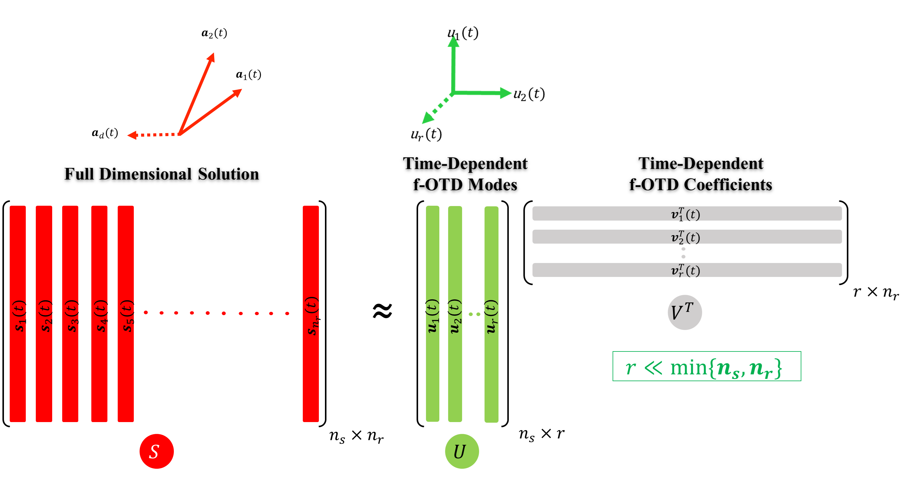
Figure 1: Modeling sensitivity matrix $S(t)$ as a multiplication of two low-ranked matrices $U(t)$ and $Y(t)$ which evolve according Eq. (5). Reprinted from Nouri et al. (2022) with permission.

The model reduction strategy is based on selecting reactions, whose perturbations grow most intensely in the abundance Eq. (2). The selection of important reactions is performed by instantaneous observation of modeled sensitivities. In f-OTD, the sensitivity matrix $S(t)$ is modeled by factorizing it into a time-dependent subspace in the $n_{s}$-dimensional phase space of abundances represented by a set of f-OTD modes: $U(t)=[\mbox{\boldmath$u$}_{1}(t),\mbox{\boldmath$u$}_{2}(t),\dots,\mbox{\boldmath$u$}_{r}(t)]\in\mathbb{R}^{n_{s}\times r}$. These modes are orthonormal $\mbox{\boldmath$u$}_{i}^{T}(t)\mbox{\boldmath$u$}_{j}(t)=\delta_{ij}$ at all $t$, where $\delta_{ij}$ is the Kronecker delta. The rank of $S(t)\in\mathbb{R}^{n_{s}\times n_{r}}$ is $d=\mbox{min}\{n_{s},n_{r}\}$ while the f-OTD modes represent a rank-$r$ subspace, where $r\ll d$. To this end, the sensitivity matrix is approximated via the f-OTD decomposition (Fig. 1) as $S(t)\approx U(t)V^{T}(t)$ where $V(t)=[\mbox{\boldmath$v$}_{1}(t),\mbox{\boldmath$v$}_{2}(t),\dots,\mbox{\boldmath$v$}_{r}(t)]\in\mathbb{R}^{n_{r}\times r}$ is the f-OTD coefficient matrix. This decomposition is a low-rank approximation of the sensitivity matrix $S(t)$. Therefore, $U(t)V(t)^{T}$ closely approximates $S(t)$ and it is not exact. Both $U(t)$ and $V(t)$ are time-dependent, and their explicit time dependency on $t$ is dropped for brevity. Figure 1 shows the schematic of the decomposition of $S$ into f-OTD components $U$ and $V$. The evolution equation for $U$ and $V$ are obtained by substituting the sensitivity decomposition ($S(t)\approx U(t)V^{T}(t)$) into Eq. (4):

$$\frac{dU}{dt} = QLU+QFVC^{-1},$$ (5a)

$$\frac{dV}{dt} = VL_{r}^{T}+F^{T}U,$$ (5b)

where $Q=I-UU^{T}$ is the orthogonal projection onto the space spanned by the complement of $U$ and $C=V^{T}V\in\mathbb{R}^{r\times r}$ is a correlation matrix. Matrix $C(t)$ is, in general, a full matrix implying that the f-OTD coefficients are correlated. $L_{r}=U^{T}LU\in\mathbb{R}^{r\times r}$ is a reduced linearized operator. Equation (5) represents a coupled system of ODEs and constitutes the f-OTD evolution equations. The f-OTD modes align themselves with the most instantaneously sensitive directions of the abundance evolution equation when perturbed by $\alpha$. It is shown by Babaee et al. (2017b) that when $\alpha$ is the perturbation to the initial condition, the OTD modes converge exponentially to the eigen-directions of the Cauchy–Green tensor associated with the most intense finite-time instabilities.

The primary computational advantage of using f-OTD is that the method only evolves two skinny matrices containing $(n_{s}+n_{r})\times r$ elements as opposed to $n_{s}\times n_{r}$ elements in the SE (Eq. (4)). This reduces the required memory for ODE solvers drastically and facilitates the application of stiff solvers for evolving sensitivities. Moreover, in the f-OTD decomposition, the sensitivities are stored in the compressed form, i.e., matrices $U$, and $V$ are kept in the memory as opposed to their multiplication $UV^{T}$, i.e., the decompressed form. Therefore, in comparison to the full SE, f-OTD decomposition results in the memory compression ratio of $(n_{s}\times n_{r})/((n_{s}+n_{r})r)$.

2.2 Identification of important reactions & isotopes

In f-OTD skeletal reduction, modeled sensitivities are computed in a factorized format by solving Eqs. (2), (5a), and (5b), and the values of $U$, $V$, and $\mathbf{y}$ are stored at resolved time steps $t_{i}\in[0,t_{f}]$. Equation  (2) is initialized with different sets of isotope abundances, temperature and density within their ranges of interest. Each simulation with a different initial condition is identified as a case. At each resolved time step and for each case, the eigen decomposition of $S^{T}S\in\mathbb{R}^{n_{r}\times n_{r}}$ is computed as $A\Lambda A^{T}$, and the vector $\mbox{\boldmath$w$}=(\Sigma\lambda_{i}|\mbox{\boldmath$a$}_{i}|)/(\Sigma\lambda_{i})\in\mathbb{R}^{n_{r}}$ is basically the average of eigenvectors of $S^{T}S$ matrix weighted based on their associated eigenvalues ($\lambda_{i}$), and prevents dealing with each eigenvector ($\mbox{\boldmath$a$}_{i}$) separately. Each component of $w$, i.e. $w_{i}$, is positive and associated with a certain reaction ($i$th reaction). The larger the $w_{i}$ value, the more important the reaction $i$ is. The $w_{max,i}$ denotes the highest value of $w_{i}$ through all resolved time steps and cases. The elements of $\mbox{\boldmath$w$}_{max}$ vector are sorted in descending order to find the indices of the most important reactions in the detailed model. Isotopes are also sorted based on their first presence in the sorted reactions, i.e. isotopes which first show up in a higher ranked reaction would be more important than an isotope which first participates in a lower ranked reaction. This results in a reaction and isotope ranking based on $\mbox{\boldmath$w$}_{max}$ vector. Finally, a set of isotopes are chosen by defining a threshold $\epsilon$ on the element of $\mbox{\boldmath$w$}_{max}$ vector and eliminating isotopes whose associated $w_{max,i}$ are less than $\epsilon$. This terminates reactions which include the eliminated isotopes from the detailed model. Since the model reduction is reaction based, any non-reactive isotope with a non-zero mass fraction in the initial condition must be manually added to the skeletal model.

In summary, the nuclear combustion system is instantaneously observed, and the reactions are sorted based on their effects on sensitivities to find the most important isotopes. These isotopes and the reactions which connect them together create the skeletal models. In combustion systems, perturbations with respect to “fast” reactions generate very large sensitivities for short time periods which vanish as $t\rightarrow\infty$. On the other hand, perturbations with respect to “slow” reactions generate smaller and more sustained sensitivities. The approach here is based on the instantaneous observation of sensitivities, both slow and fast reactions can leave an imprint on the instantaneous normalized reaction vector ($w$) if their imprints are larger than the threshold value ($\epsilon$). However, if the sensitivities associated with fast and slow reactions from pre-determined times and locations are combined with each other before dimension reduction, as commonly done in principal component analysis (PCA) type schemes, the smaller sensitivities associated with slow reactions would be out-weighted by the large sensitivities associated with fast reactions.

3 skeletal reduction on the Approx21 RN

The process of eliminating unimportant reactions and isotopes from a kinetics model with f-OTD is demonstrated in this section with a simple example. Let us start with the Approx21 model which is the default MESA network (Paxton et al., 2011, 2015) for alpha chain reactions. Approx21 evolves $n_{s}=21$ isotopes: $\ce{n}$, $\ce{p}$, $\ce{{}^{1}H}$, $\ce{{}^{3}He}$, $\ce{{}^{4}He}$, $\ce{{}^{12}C}$, $\ce{{}^{14}N}$, $\ce{{}^{16}O}$, $\ce{{}^{20}Ne}$, $\ce{{}^{24}Mg}$, $\ce{{}^{28}Si}$, $\ce{{}^{32}S}$, $\ce{{}^{36}Ar}$, $\ce{{}^{40}Ca}$, $\ce{{}^{44}Ti}$, $\ce{{}^{48}Cr}$, $\ce{{}^{56}Cr}$, $\ce{{}^{52}Fe}$, $\ce{{}^{54}Fe}$, $\ce{{}^{56}Fe}$, and $\ce{{}^{56}Ni}$ through $n_{r}=112$ reactions. In this RN, ($\alpha$,p)(p,$\gamma$) and ($\gamma$,p)(p,$\alpha$) links are included in order to obtain reasonably accurate energy generation rates and abundance levels when the temperature exceeds 2.5e9 K. At these elevated temperatures, the flows through the ($\alpha$,p)(p,$\gamma$) sequences are faster than the flows through the ($\alpha$,$\gamma$) channels. An ($\alpha$,p)(p,$\gamma$) sequence is, effectively, an ($\alpha$,$\gamma$) reaction through an intermediate isotope. By assuming steady-state proton flows through intermediate isotopes $\ce{{}^{27}Al}$, $\ce{{}^{31}P}$, $\ce{{}^{35}Cl}$, $\ce{{}^{39}K}$, $\ce{{}^{43}Sc}$, $\ce{{}^{47}V}$, $\ce{{}^{51}Mn}$, and $\ce{{}^{55}Co}$, this strategy avoids explicitly evolving the abundances of the proton or intermediate isotopes. The skeletal reduction is exemplified here by analyzing only one case for the constant-$\rho T$ burning of a mixture of carbon and oxygen in a WD progenitor.

Figure 2: Model reduction for Approx21: eigenvalues of the $S^{T}S$ matrix. The sensitivity matrix, $S$, initially evolves exactly via the SE (Eq. (4)), and then evolves approximately with the f-OTD equations (Eq. (5)). The f-OTD simulation ($t>10^{-9}$) only evolves $r$ modes of the full order model ($t<10^{-9}$). Ignition data is gathered from the constant-$\rho T$ burning simulation case described in Fig. 3.

The ignition initiates with $T_{9}=3$, $\rho_{9}=1$, and $\mathtt{x}_{C,0}=\mathtt{x}_{O,0}=0.5$, so $\mathtt{y}_{e}=0.5$. Here, $T_{9}\equiv T/(10^{9}K)$ and $\rho_{9}\equiv\rho/(10^{9}g.cm^{-3})$. The sensitivities evolve in two phases. In the first, the full-dimensional SE (Eq. (4)) is solved for a very small time period, e.g. until $t=10^{-12}s$, to generate the initial conditions for the f-OTD simulation. In the second phase, the sensitivity matrix ($S$) is approximated by evolving the f-OTD equations (Eq. (5)). The $U$ and $Y$ matrices are initialized by eigenvalue decomposition of the full sensitivity matrix ($S$) at the end of the first phase. Figure 2 shows the evolution of the eigenvalues of $S^{T}S$ matrix. It is indicated that $i$) $\lambda_{1}$ is an order of magnitude larger than $\lambda_{2}$ most of the time, and $ii$) the modeled sensitivities converge by adding more modes. Therefore, f-OTD simulation with $r=1$ provides a reasonable estimation of sensitivities, which is enough if the final goal is to determine the importance of reactions/isotopes.

Figure 3 shows the ranking of reactions and isotopes in Approx21 associated with the constant-$\rho T$ burning case. It is apparent that reactions 4 ($\ce{{}^{12}C}$($\ce{{}^{12}C}$,$\alpha$)$\ce{{}^{20}Ne}$), equilibrium reactions 92 ($\ce{{}^{24}Mg}$($\alpha$,p)$\ce{{}^{27}Al}$(p,$\gamma$)$\ce{{}^{28}Si}$), 93 ($\ce{{}^{28}Si}$($\alpha$,p)$\ce{{}^{31}P}$(p,$\gamma$)$\ce{{}^{32}S}$), and 95 ($\ce{{}^{36}Ar}$($\alpha$,p)$\ce{{}^{39}K}$(p,$\gamma$)$\ce{{}^{40}Ca}$), and reaction 6 ($\ce{{}^{16}O}$($\ce{{}^{16}O}$,$\alpha$)$\ce{{}^{28}Si}$) are the first five most important reactions, and isotopes $\ce{{}^{4}He}$, $\ce{{}^{12}C}$, $\ce{{}^{20}Ne}$, $\ce{{}^{24}Mg}$, and $\ce{{}^{28}Si}$ are the first five most important isotopes in Approx21 for the ignition case considered.

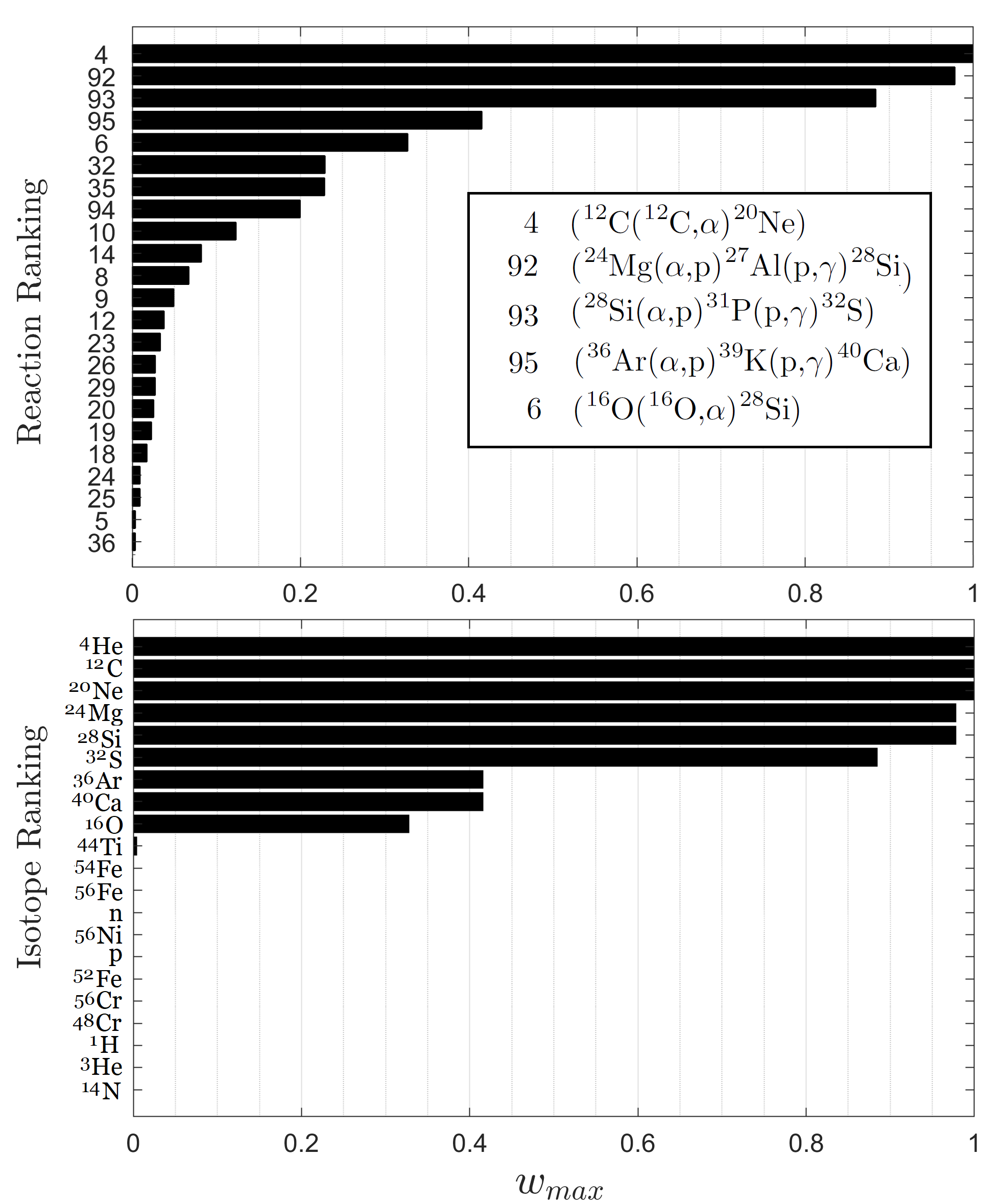
Figure 3: Model reduction for Approx21: reaction and isotope ranking based on their associated $w_{max}$ from one constant-$\rho T$ burning simulation case with $T_{9}=3$, $\rho_{9}=3$, and initial composition of $\mathtt{x}_{C,0}=\mathtt{x}_{O,0}=0.5$ with $\mathtt{y}_{e,0}=0.5$.

The f-OTD-10 model is then created based on the algorithm described in §2.2 and contains 10 most important isotopes shown in Fig. 3, i.e., $\ce{{}^{4}He}$, $\ce{{}^{12}C}$, $\ce{{}^{20}Ne}$, $\ce{{}^{24}Mg}$, $\ce{{}^{28}Si}$, $\ce{{}^{32}S}$, $\ce{{}^{36}Ar}$, $\ce{{}^{40}Ca}$, $\ce{{}^{16}O}$, and $\ce{{}^{44}Ti}$. Approx13 (Timmes et al. (2000)) is a 13 isotope ($\ce{{}^{4}He}$, $\ce{{}^{12}C}$, $\ce{{}^{16}O}$, $\ce{{}^{20}Ne}$, $\ce{{}^{23}Mg}$, $\ce{{}^{28}Si}$, $\ce{{}^{32}S}$, $\ce{{}^{36}Ar}$, $\ce{{}^{40}Ca}$, $\ce{{}^{44}Ti}$, $\ce{{}^{48}Cr}$, $\ce{{}^{52}Fe}$, and $\ce{{}^{56}Ni}$) reaction network which is also extracted from Approx21 but over a wider time range to produce $\ce{{}^{56}Ni}$. That is why Approx13 contains three more isotopes, i.e. $\ce{{}^{48}Cr}$, $\ce{{}^{52}Fe}$, and $\ce{{}^{56}Ni}$ in comparison with f-OTD-10. Nevertheless, this simple exercise demonstrates the ability of f-OTD methodology to extract the relevant isotopes for a given set of conditions and starting RN. Figure 4 demonstrates the performance of f-OTD-10 RN in predicting the evolution of isotope mass fractions over its design conditions ($T_{9}=3$, $\rho_{9}=1$, $\mathtt{x}_{C,0}=\mathtt{x}_{O,0}=0.5$, and $t\in[0,10^{4}]s$).

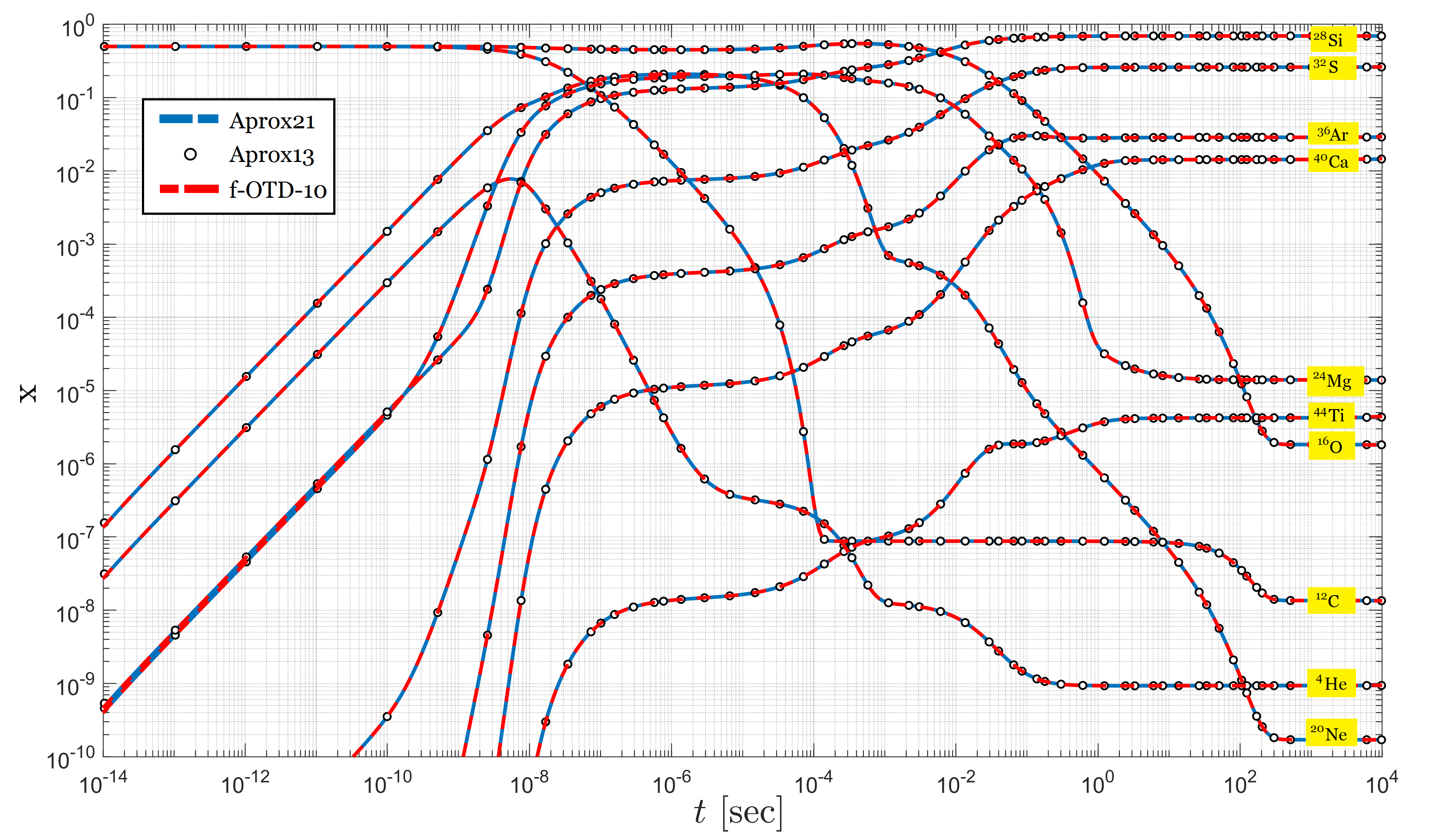
Figure 4: Model reduction for Approx21: evolution of isotope mass fractions based on Approx21, Approx13, and f-OTD-10. The last two models are generated from Approx21.

4 Skeletal reduction on the Torch RN

In SNe Ia, the carbon and oxygen burn together to produce nuclei from silicon to the iron peak which are being ejected into the interstellar medium (Nomoto, 1997; Woosley et al., 2002; Lippuner & Roberts, 2017; Johnson, 2019). As this type of supernova does not produce a significant amount of free neutrons, it does not synthesize elements beyond the iron peak (Johnson, 2019). Nevertheless, some heavier isotopes can contribute to reactions involving isotopes important to light curves observations, such as $\ce{{}^{56}Ni}$. The 495-isotope version of the Torch RN (Paxton et al., 2015) is chosen to represent the detailed RN in this section. The Torch RN extends from $\ce{{}^{1}H}$ to $\ce{{}^{91}Tc}$ (Timmes, 1999) with $n_{s}=495$ and $n_{r}=6012$. The weak reactions are turned on, and no screening is performed on the reaction rates (Fuller et al., 1985). The Helmholtz EOS as developed by Timmes & Swesty (2000) is used with Coulomb correction to calculate the internal energy and the pressure. Several skeletal RNs have been previously proposed based on the Torch model for inline calculations (Timmes, 1999; Timmes & Swesty, 2000; Anninos et al., 2019) and are used in the MESA code (Paxton et al., 2011; Anninos et al., 2019; Paxton et al., 2015). These include a bare minimum model of the $\alpha$-chain reactions using 13 isotopes, a 19-isotope RN to also accommodate some hydrogen burning (Weaver et al., 1978), and a 21-isotope RN that adds ⁵⁶Cr and ⁵⁶Fe and respective equilibrium reaction sequences to the 19 isotope network to attain a lower $\mathtt{y}_{e}$ value for pre-supernova models (Paxton et al., 2015). Several important isotopes are produced in burning scenarios with $\mathtt{y}_{e}$ significantly lower than $0.5$. For example, Woosley (1997) suggests that ⁴⁸Ca can only be produced in nature in a subset of SNe Ia, with $\mathtt{y}_{e}$ in the range $0.41$ to $0.42$ and high burning density. The Torch RN covers such scenarios. On the other hand, the performances of the existing skeletal models have not been systematically examined to cover both $\mathtt{y}_{e}=0.5$ and $\mathtt{y}_{e}<0.5$ scenarios. This is addressed here by considering initial conditions with different $\mathtt{y}_{e}$ values and choosing the 21-isotope RN skeletal model (hereafter denoted Approx21) for comparison with the proposed skeletal RNs.

The SNe Ia progenitor population and burning scenarios cover a wide range of temperatures and densities (Hillebrandt & Niemeyer, 2000) so that, most likely, a single skeletal model with a limited number of isotopes ($n_{s}$) cannot yield accurate predictions over the full range of conditions which would be covered by a detailed RN. Because of the importance of ${}^{56}\text{Ni}$ in SNe Ia, the skeletal models in this work are designed to predict the evolution of $\mathtt{x}_{{}^{56}\text{Ni}}$ correctly. For this purpose, a map of maximum production of this isotope is produced during the course of constant-$\rho T$ burning in SNe Ia as shown in Fig. 5. The Torch RN is run 10000 times on a 100$\times$100 grid of $T_{9}$ and $\rho_{9}$ for $\mathtt{y}_{e,0}$ values of 0.4955 and 0.5. It is observed that ${}^{56}\text{Ni}$ is only significantly produced within certain ranges of the temperature and the density values, with a noticeable shift of the ${}^{56}\text{Ni}$ production near the peak. In particular, the peak occurs around $T_{9}=4.0$ at lower densities. Moreover, the maximum production of ${}^{56}\text{Ni}$ is decreased by decreasing $\mathtt{y}_{e,0}$ (Iliadis, 2015). To generate skeletal reactions, simulations are conducted of constant-$\rho T$ burning in SNe Ia for 24 cases, with $T_{9}\in\{2,4,6\},\rho_{9}\in\{0.001,0.01,0.1,1.0\}$, and $\mathtt{y}_{e,0}\in\{0.4955,0.5\}$. To better show how these cases are distributed, a 2D version of Fig. 5 is shown in Fig. 6. Each case (shown as a red circle in Fig. 6) denotes a set of initial condition for the density, the temperature, the energy and isotope mass fractions. These conditions cover the burning stage, and are of interest in multidimensional simulations (Fryxell et al., 2000; Woosley et al., 2007).

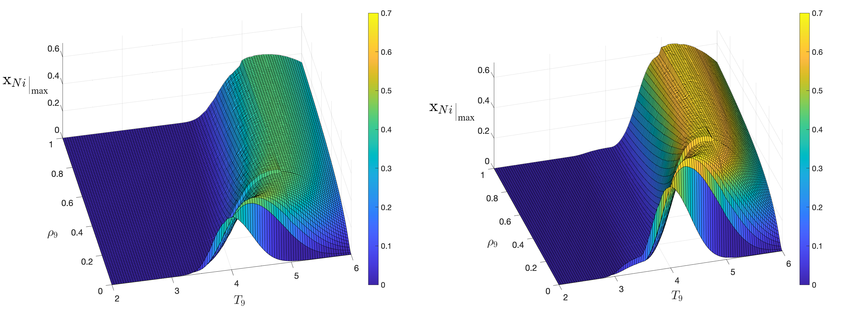
Figure 5: Maximum mass fraction of ${}^{56}\text{Ni}$ during constant-$\rho T$ burning of SNe Ia. Red circles show the f-OTD cases.

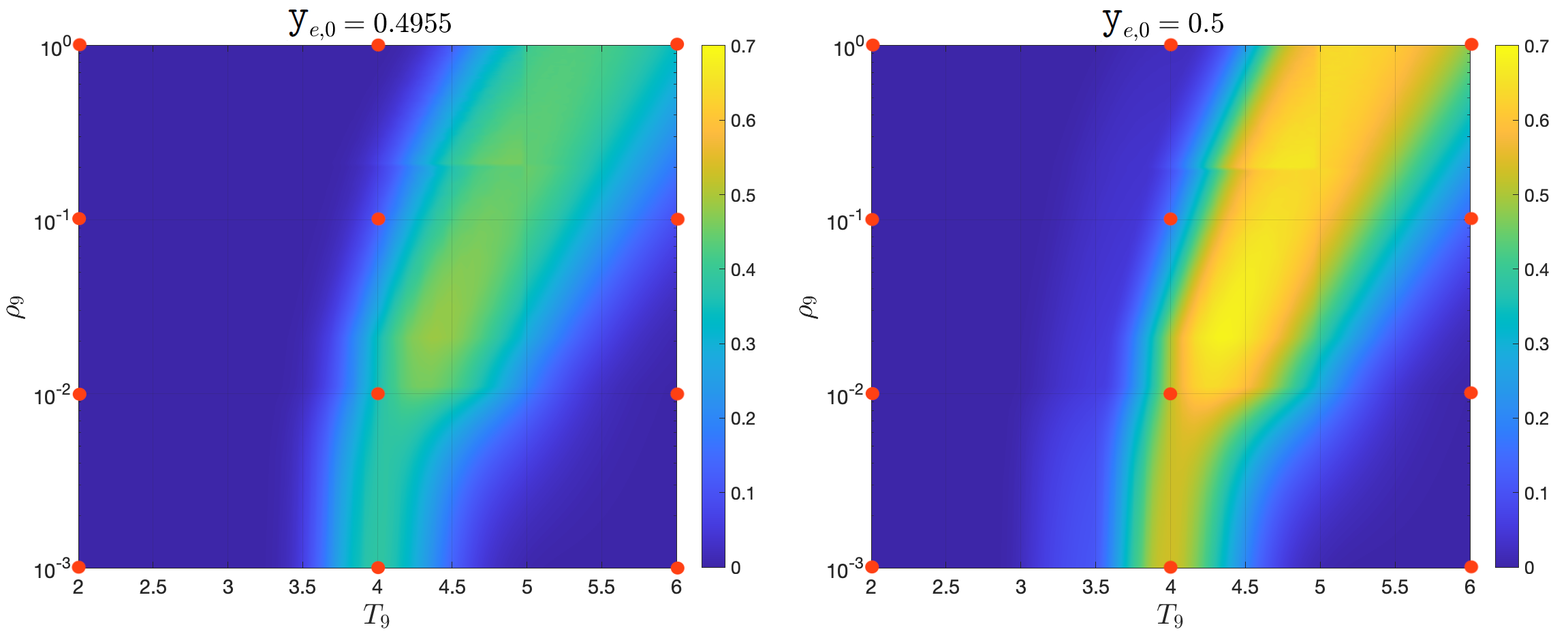
Figure 6: Maximum mass fraction of ${}^{56}\text{Ni}$ during constant-$\rho T$ burning of SNe Ia. Red circles show the f-OTD cases.

The final time for each case is when the mass fraction of ${}^{56}\text{Ni}$ reaches its maximum. Figure 7 shows the evolution of isotope mass fractions for two different cases. The red lines in Fig. 7 show the ${}^{56}\text{Ni}$ mass fraction and blue triangles denote the final time of f-OTD simulations and sensitivity analysis. The initial mass fractions of $\ce{{}^{12}C}$, $\ce{{}^{16}O}$, and $\ce{{}^{22}Ne}$ isotopes in cases with $\mathtt{y}_{e,0}=0.5$ are $\mathtt{x}_{C,0}=\mathtt{x}_{O,0}=0.5$, and in cases with $\mathtt{y}_{e,0}=0.4955$ are $\mathtt{x}_{C,0}=0.45$, $\mathtt{x}_{O,0}=0.45$, and $\mathtt{x}_{Ne,0}=0.1$. Note that for the conditions considered here, the sharp decline in ${}^{56}\text{Ni}$ mass fraction at $t\gtrsim 10s$ is likely due to electron capture, causing the network composition to shift to more neutron-rich isotopes of nickel and iron, which is not really relevant to carbon/oxygen burning and therefore not used in the f-OTD analysis. The f-OTD method is used to model the sensitivity matrix with $r=1$ mode, and the generated skeletal models by sensitivity analysis are denoted by f-OTD-n in which “n” identifies for the number of isotopes. The predictive capabilities of f-OTD models are compared against those obtained via Torch RN and the Approx21.

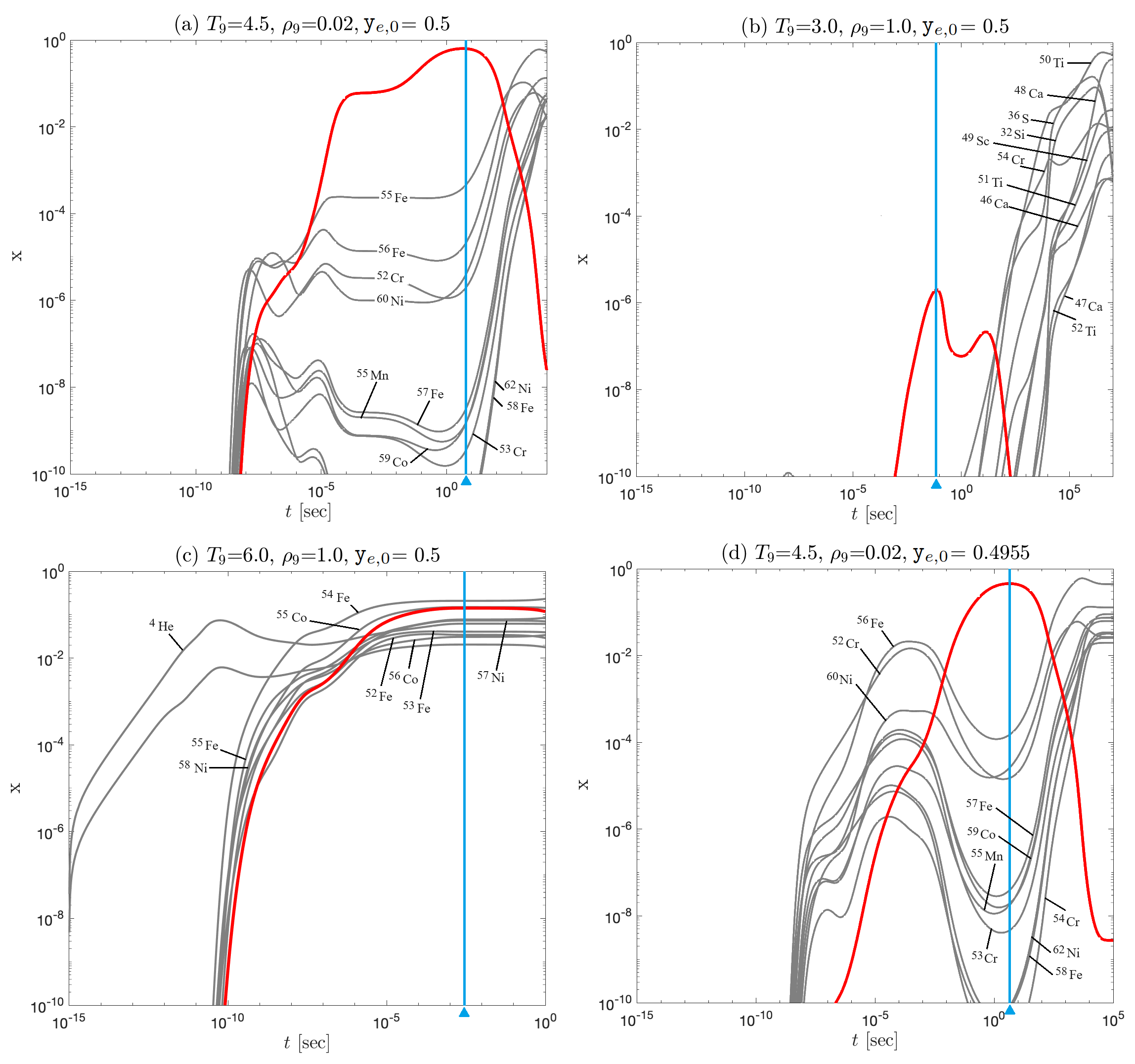
Figure 7: Evolution of isotope mass fractions in Torch with different initial conditions, highlighting different scenarios for $\ce{{}^{56}Ni}$ evolution. The blue lines indicate the final time of the f-OTD simulations and sensitivity analysis. The red and gray lines represent the $\ce{{}^{56}Ni}$ mass fraction and the 10 isotopes with the highest final mass fractions observed during the portrayed ignition process. These isotopes are listed in the left-top corner of each sub-figure

A ranking is provided of the first 150 important isotopes in Appendix A considering the maximum characteristic value associated with each isotope, i.e. $w_{max,i}$. Different skeletal models can be generated by applying a threshold $\epsilon$ on $\mbox{\boldmath$w$}_{max}$ and eliminating isotopes and their associated reactions with $w_{max,i}<\epsilon$ from Torch RN. A comprehensive skeletal model capable of reproducing the energy and isotope mass fraction predictions of Torch RN with a certain accuracy can be developed by specifying an acceptable error level, e.g. 5%, in energy or ${}^{56}\text{Ni}$ mass fraction estimations. Figure 8(a) shows the isotopes in Torch selected for the f-OTD-150. Each square belongs to an isotope, and isotopes with darker colors are ranked higher (selected earlier) than isotopes with lighter colors. The results show at least 114 isotopes are required to accurately produce ${}^{56}\text{Ni}$ with a f-OTD skeletal model. This is because of the importance of some isotopes with $21\leq N,Z\leq 24$, and especially ${}^{43}\text{Sc}$ in bridging between lighter and heavier isotopes and two QSE clusters (Iliadis, 2015; Subedi et al., 2020). It is shown in Fig. 8(a) that ${}^{43}\text{Sc}$ plays a key role for proton and neutron channels. Figures 8(b) and 8(c) show the isotopes used in the Approx21 model and SK55, a skeletal model used by Townsley et al. (2019).

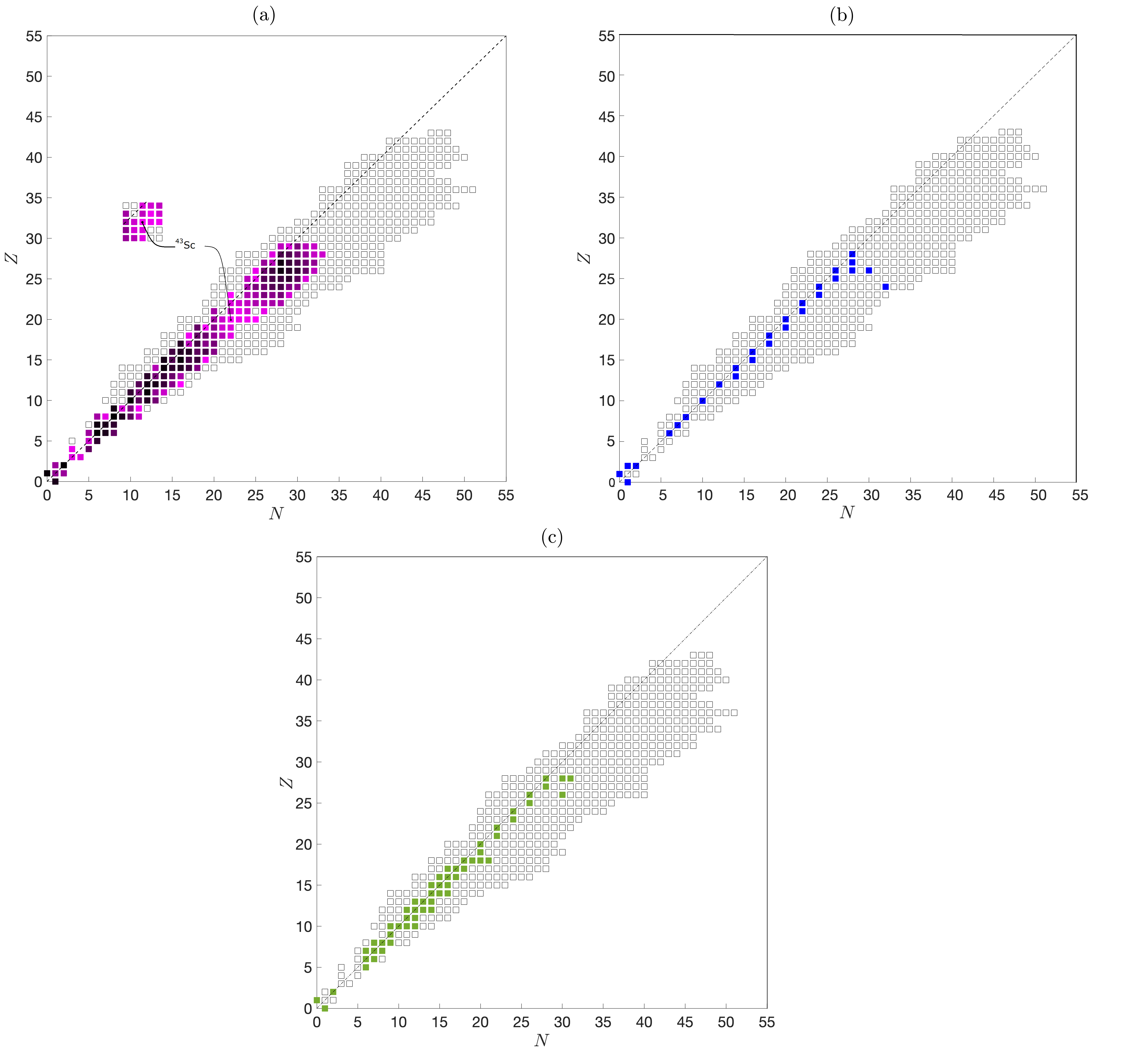
Figure 8: (a) The first 150 ranked isotopes of Torch RN sufficient for exact calculation of the maximum $\ce{{}^{56}Ni}$ abundance and energy in SNe Ia. The darker the squares, the more important (higher ranked) isotopes and the empty squares correspond to eliminated isotopes from the Torch RN. The ${}^{43}\text{Sc}$ is a key isotope in proton and neutron channels toward ${}^{56}\text{Ni}$ production. The f-OTD models with less than 114 isotopes (Appendix A) do not contain ${}^{43}\text{Sc}$ and do not produce the correct amount of ${}^{56}\text{Ni}$. (b) The isotopes for Approx21 and (c) SK55.

The Torch RN is user friendly and flexible to work with any subset of its own isotopes. This means that by providing a ranked list of isotopes from Appendix A, e.g. $\ce{{}^{16}O}$ (1^st rank) to $\ce{{}^{45}Ca}$ (150^th rank), one can use a f-OTD generated network with the associated isotopes. Figures 9 & 10 show the performance of the f-OTD models in reproducing the energy, mass fractions of ${}^{12}\text{C}$, ${}^{44}\text{Ti}$, and ${}^{56}\text{Ni}$, and $\mathtt{y}_{e}$. The radioactive decays of ${}^{44}\text{Ti}$, and ${}^{56}\text{Ni}$ have significant observational applications, and the production of these two isotopes is sensitive to the temperature, density, and $\mathtt{y}_{e}$ evolution (Magkotsios et al. (2010)). The energy in Fig. 10 is normalized by its initial value. The predictions via the Approx21 and SK55 are also presented. The second and third row of subfigures correspond to situations exactly similar to the test cases, but the first and last rows portray the estimations for arbitrary situations within the initial condition domain, i.e., $T_{9}\in[2,6]$, $\rho_{9}\in[0.001,1.0]$, and $\mathtt{y}_{e,0}\in[0.4955,0.5]$. It is apparent that the f-OTD models with $n_{s}\geq 150$ exactly predict the energy evolution of Torch RN and ${}^{56}\text{Ni}$ mass fraction within their designed $\rho_{9}$-$T_{9}$-$\mathtt{y}_{e}$ ranges. The Approx21 and SK55 models usually over-predict the maximum ${}^{56}\text{Ni}$ mass fraction, and Approx21 cannot be used when $\mathtt{y}_{e,0}\neq 0.5$. Replacing Torch with f-OTD models using 114-150 isotopes yields compression ratios ranging from 3.3 to 4.3. Figure 11 compares the evolution of mass fractions as predicted by Torch model, without any approximation, and nuclear statistical equilibrium (NSE) assumption. The NSE results are generated by using the instantaneous values of $\rho_{9}$-$T_{9}$-$\mathtt{y}_{e}$ extracted from non-NSE calculations. The Torch and f-OTD-150 are used as the base reaction network for NSE estimations. It is shown in Figs. 11(a) & (b) that only at late time for $T_{9}=5$ the NSE and non-NSE mass fraction predictions of ${}^{44}\text{Ti}$ and ${}^{56}\text{Ni}$ (but not ${}^{12}\text{C}$) are close to each other.

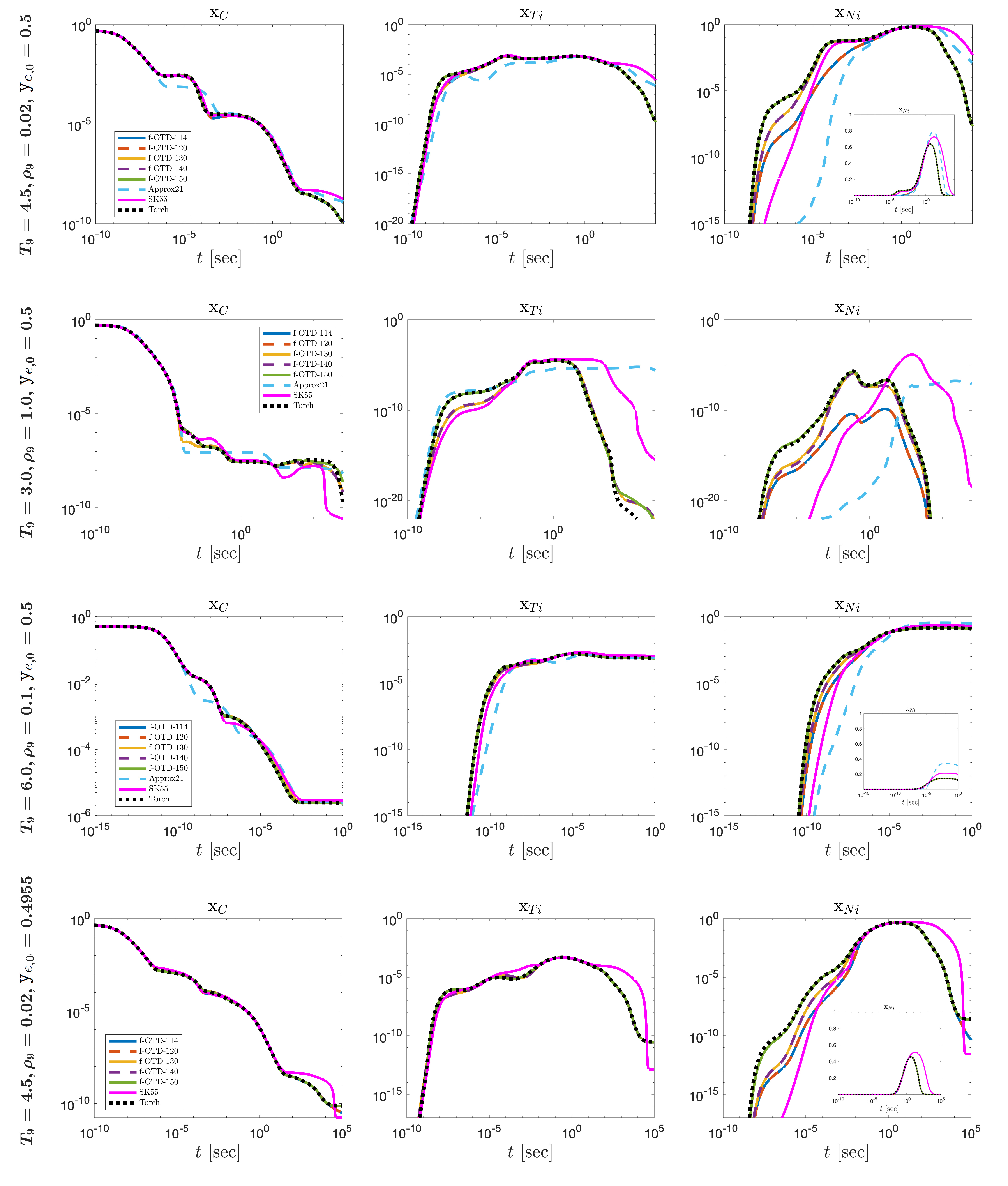
Figure 9: Model reduction on Torch RN: mass fraction estimations via Torch RN, Approx21, SK55, and f-OTD generated models for four different initial conditions of $\mathtt{x_{c12}}$, $\mathtt{x_{o16}}$, $T_{9}$, and $\rho_{9}$.

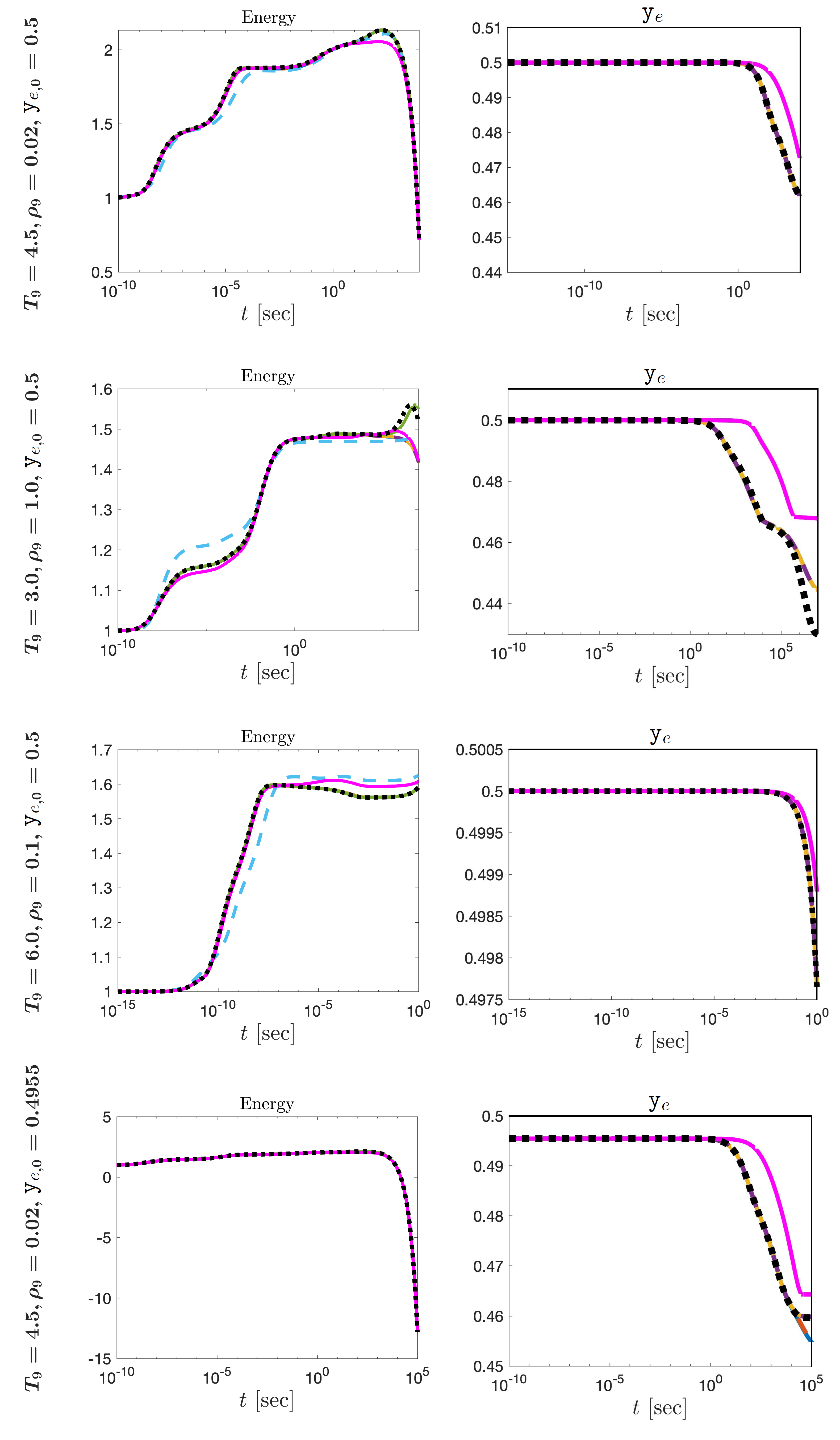
Figure 10: Model reduction on Torch RN: energy and $\mathtt{y}_{e}$ estimations via Torch RN, Approx21, SK55, and f-OTD generated models for four different initial conditions of $\mathtt{x_{c12}}$, $\mathtt{x_{o16}}$, $T_{9}$, and $\rho_{9}$.

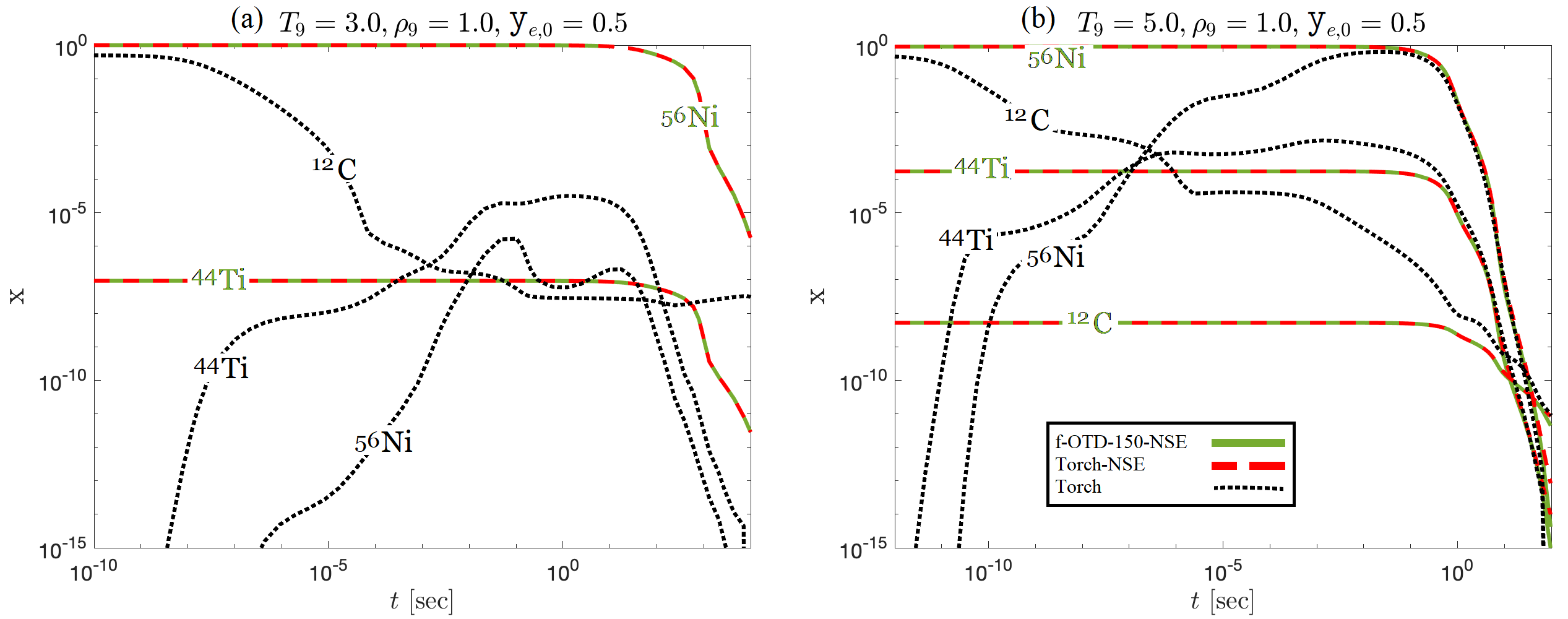
Figure 11: Comparison between mass fractions as predicted by Torch model (black dotted lines) without any equilibrium assumptions and NSE mass fractions estimated based on Torch and f-OTD-150 models (green solid and red dashed lines). NSE and non-NSE simulations have same $\mathtt{y}_{e}$ at each time.

5 Conclusions

A systematic method for skeletal model reduction of nuclear reaction networks is developed for generating models for the carbon-oxygen combustion in SN Ia covering a range of temperatures and electron number fraction, $\mathtt{y}_{e}=Z_{m}/A_{m}$. In this method, the sensitivities of abundances with respect to reaction rates are modeled using the forced optimally time-dependent (f-OTD) method and are analyzed instantaneously. This results in reaction and isotope rankings based on the correlations between their sensitivities. A key feature of this approach is that it factorizes the sensitivity matrix into a multiplication of two low-ranked time-dependent matrices which evolve based on evolution equations derived from the governing equations of the system. The generated skeletal models are comparatively assessed based on their ability to predict the energy and mass fractions. In particular, the skeletal models as derived here are the first to address situations covering both $\mathtt{y}_{e}=0.5$ and $\mathtt{y}_{e}<0.5$. To employ any of the skeletal models developed in this work or to create new f-OTD skeletal models with different numbers of isotopes, one only needs to feed a list of more than 114 ranked isotopes from Appendix A into the Torch RN. Further reduction in the number of isotopes (e.g., by using equilibrium assumptions) is a potential future follow-up to this work.

The overall costs of generating an f-OTD model depend on solving the mass fraction equations (which is roughly the same as one non-f-OTD Torch simulation, $c_{torch}$), the $U$ equation, whose cost scales as $r\times c_{torch}$, and $V$ equation, whose cost scales as $r\times n_{r}/n_{s}\times c_{torch}$. For example, the total cost to generate the f-OTD-150 model with $r=1$ modes, for which 10 cases with different densities and temperatures were used, was $\sim 120c_{torch}$, which would be negligible, for example, compared to a Monte Carlo simulation with $\sim 10,000$ trials. On the other hand, f-OTD-150 should run $\sim 3.3$ faster than Torch.

The skeletal reduction technique as described here can be readily extended to other situations. For example, lower values of $\mathtt{y}_{e}$ and higher densities to examine the production of ⁴⁸Ca, ⁵⁰Ti, or ⁵⁴Cr. It can also be applied to more complex RNs to examine the production of heavier elements in core-collapse supernovae. With respect to the development of the methodology itself, it can be extended by including the sensitivity analysis based also on transport properties, or even the equation of state (Nouri et al., 2019). Most importantly, as shown recently (Donello et al., 2022), the f-OTD methodology can be used for solving PDEs for multi-dimensional combustion problems in a cost-effective manner — by exploiting the correlations between the spatiotemporal sensitivities of different species with respect to different parameters. This analysis can be especially insightful for problems containing rare events by providing more insights into global phenomena.

Appendix A Isotope ranking based on all cases ($\mathtt{y}_{{e},0}\leq 0.5$)

Rank	Isotope	$w_{max}$	Rank	Isotope	$w_{max}$	Rank	Isotope	$w_{max}$	Rank	Isotope	$w_{max}$
1	16O	0.967	41	32P	0.112	81	27Mg	0.020	121	61Ni	0.003
2	20Ne	0.967	42	35Cl	0.105	82	50V	0.018	122	45Sc	0.002
3	4He	0.967	43	52Cr	0.094	83	54Cr	0.018	123	45Ti	0.002
4	12C	0.935	44	52Mn	0.094	84	39K	0.016	124	40K	0.002
5	23Na	0.796	45	56Ni	0.094	85	24Na	0.014	125	52V	0.002
6	p	0.796	46	35S	0.093	86	2H	0.014	126	18F	0.002
7	31P	0.761	47	57Co	0.085	87	59Co	0.012	127	44Ti	0.002
8	28Si	0.743	48	57Ni	0.085	88	59Ni	0.012	128	56Mn	0.001
9	13N	0.732	49	30P	0.083	89	53Co	0.011	129	58Cu	0.001
10	54Fe	0.707	50	51Cr	0.081	90	38Ar	0.011	130	7Li	0.001
11	55Co	0.707	51	51Mn	0.081	91	3H	0.010	131	41K	0.001
12	17F	0.704	52	23Mg	0.076	92	3He	0.010	132	55Ni	0.001
13	29P	0.681	53	21Ne	0.075	93	11C	0.010	133	6Li	0.001
14	24Mg	0.669	54	18O	0.066	94	40Ca	0.009	134	15O	0.001
15	25Mg	0.669	55	34S	0.066	95	41Sc	0.009	135	40Ar	0.001
16	n	0.669	56	55Mn	0.066	96	14O	0.009	136	47Sc	0.001
17	13C	0.667	57	9Be	0.066	97	48V	0.009	137	50Mn	0.001
18	14N	0.624	58	14C	0.061	98	48Cr	0.009	138	51Fe	0.001
19	17O	0.624	59	36Ar	0.052	99	49Ti	0.008	139	7Be	0.001
20	30Si	0.518	60	37K	0.052	100	29Al	0.007	140	35Ar	0.001
21	33S	0.518	61	57Fe	0.052	101	50Ti	0.007	141	43Ca	0.001
22	22Ne	0.447	62	52Fe	0.051	102	47Ti	0.007	142	44Ca	0.001
23	32S	0.441	63	28Al	0.048	103	47V	0.007	143	44Sc	0.001
24	33Cl	0.441	64	37Ar	0.046	104	48Ti	0.007	144	34P	0.001
25	25Al	0.385	65	50Cr	0.044	105	27Si	0.006	145	38K	0.001
26	55Fe	0.352	66	58Co	0.042	106	39Ar	0.006	146	42Ca	0.001
27	29Si	0.330	67	58Ni	0.042	107	54Co	0.005	147	20F	0.001
28	11B	0.295	68	23Ne	0.042	108	60Cu	0.005	148	45V	0.001
29	15N	0.285	69	51V	0.040	109	34Cl	0.005	149	28Mg	0.001
30	21Na	0.264	70	37Cl	0.040	110	49Mn	0.005	150	45Ca	0.001
31	54Mn	0.191	71	26Al	0.038	111	57Cu	0.004
32	27Al	0.177	72	22Na	0.033	112	58Fe	0.004
33	56Fe	0.163	73	49V	0.030	113	46Ti	0.004
34	56Co	0.163	74	49Cr	0.030	114	43Sc	0.004
35	26Mg	0.161	75	59Cu	0.027	115	10B	0.004
36	33P	0.155	76	53Cr	0.027	116	60Ni	0.003
37	31Si	0.142	77	19F	0.025	117	61Cu	0.003
38	53Mn	0.128	78	32Si	0.024	118	25Na	0.003
39	53Fe	0.128	79	36S	0.022	119	19O	0.003
40	31S	0.124	80	36Cl	0.022	120	41Ca	0.003

References

- Aitzhan et al. (2022) Aitzhan, A., Nouri, A., Givi, P., & Babaee, H. 2022, arXiv preprint arXiv:2201.02097
- Anninos et al. (2019) Anninos, P., Hoffman, R., Grewal, M., Lavell, M., & Fragile, P. 2019, Astrophys. J., 885, 136
- Arnett (1996) Arnett, W. D. 1996, Supernovae and Nucleosynthesis: An Investigation of the History of Matter, from the Big Bang to the Present (Princeton University Press)
- Arnould & Goriely (2020) Arnould, M., & Goriely, S. 2020, Prog. Part. Nucl. Phys., 112, 103766
- Babaee (2019) Babaee, H. 2019, Proc. R. Soc. Lond. A, 475, 20190506
- Babaee et al. (2017a) Babaee, H., Choi, M., Sapsis, T., & Karniadakis, G. 2017a, J. Comput. Phys., 344, 303
- Babaee et al. (2017b) Babaee, H., Farazmand, M., Haller, G., & Sapsis, T. P. 2017b, Chaos: An Interdisciplinary Journal of Nonlinear Science, 27, 063103, doi: 10.1063/1.4984627
- Barnes et al. (2021) Barnes, J., Zhu, Y., Lund, K., et al. 2021, The Astrophysical Journal, 918, 44
- Beaudet & Reeves (1983) Beaudet, G., & Reeves, H. 1983, in Primordial Helium, 53–63
- Bliss et al. (2020) Bliss, J., Arcones, A., Montes, F., & Pereira, J. 2020, Physical Review C, 101, 055807
- Bodansky et al. (1968) Bodansky, D., Clayton, D., & Fowler, W. 1968, Astrophysical Journal Supplement, vol. 16, p. 299 (1968), 16, 299
- Bora et al. (2022) Bora, Z., Vinkó, J., & Könyves-Tóth, R. 2022, Publ. Astron. Soc. Pac., 134, 054201
- Bravo et al. (2019) Bravo, E., Badenes, C., & Martínez-Rodríguez, H. 2019, Mon. Not. R. Astron. Soc., 482, 4346
- Bravo & Martinez-Pinedo (2012) Bravo, E., & Martinez-Pinedo, G. 2012, Physical Review C, 85, 055805
- Cheng et al. (2013) Cheng, M., Hou, T., & Zhang, Z. 2013, J. Comput. Phys., 242, 843
- Cyburt (2004) Cyburt, R. 2004, Physical Review D, 70, 023505
- Delbourgo-Salvador et al. (1985) Delbourgo-Salvador, P., Gry, C., Malinie, G., & Audouze, J. 1985, Astronomy and Astrophysics, 150, 53
- Donello et al. (2022) Donello, M., Carpenter, M., & Babaee, H. 2022, SIAM J. Sci. Comput., 44, A128
- Fernández et al. (2017) Fernández, R., Foucart, F., Kasen, D., et al. 2017, Class. Quantum Gravity, 34, 154001
- Fryxell et al. (2000) Fryxell, B., Olson, K., Ricker, P., et al. 2000, Astrophys. J.S, 131, 273, doi: 10.1086/317361
- Fuller et al. (1985) Fuller, G., Fowler, W., & Newman, M. 1985, Astrophys. J., 293, 1
- Girimaji & Ibrahim (2014) Girimaji, S., & Ibrahim, A. 2014, Journal of Fluids Engineering, 136, 031201
- Goussis (2012) Goussis, D. 2012, Combustion Theory and Modelling, 16, 869
- Guidry & Harris (2013) Guidry, M., & Harris, J. 2013, Comput. Sci. Discov., 6, 015002
- Guidry et al. (2013) Guidry, M., Budiardja, R., Feger, E., et al. 2013, Comput. Sci. Discov., 6, 015001
- Hadi et al. (2016) Hadi, F., Janbozorgi, M., Sheikhi, M., & Metghalchi, H. 2016, Journal of Non-Equilibrium Thermodynamics, 41, 257
- Hillebrandt & Niemeyer (2000) Hillebrandt, W., & Niemeyer, J. C. 2000, Annu. Rev. Astron. Astrophys., 38, 191, doi: 10.1146/annurev.astro.38.1.191
- Hix et al. (1998) Hix, W., Khokhlov, A., Wheeler, J., & Thielemann, F. 1998, The Astrophysical Journal, 503, 332
- Hix et al. (2007) Hix, W., Parete-Koon, S., Freiburghaus, C., & Thielemann, F. 2007, The Astrophysical Journal, 667, 476
- Hix et al. (2003) Hix, W., Smith, M., Starrfield, S., Mezzacappa, A., & Smith, D. 2003, Nuclear Physics A, 718, 620
- Iliadis (2015) Iliadis, C. 2015, Nuclear Physics of Stars (John Wiley & Sons)
- Johnson (2019) Johnson, J. 2019, Science, 363, 474
- Keck (1990) Keck, J. C. 1990, Prog. Energ. Combust., 16, 125
- Khokhlov (1981) Khokhlov, A. 1981, Soviet Astronomy Letters, vol. 7, Nov.-Dec. 1981, p. 410-413. Translation. Pisma v Astronomicheskii Zhurnal, vol. 7, Dec. 1981, p. 741-747., 7, 410
- Kobayashi et al. (2020) Kobayashi, C., Karakas, A., & Lugaro, M. 2020, Astrophys. J., 900, 179
- Koch & Lubich (2007) Koch, O., & Lubich, C. 2007, SIAM Journal on Matrix Analysis and Applications, 29, 434, doi: 10.1137/050639703
- Krauss & Romanelli (1990) Krauss, L., & Romanelli, P. 1990, Astrophysical Journal, 358, 47
- Kushnir & Katz (2020) Kushnir, D., & Katz, B. 2020, Monthly Notices of the Royal Astronomical Society, 493, 5413
- Leung & Nomoto (2018) Leung, S., & Nomoto, K. 2018, Astrophys. J., 861, 143
- Li et al. (2020) Li, Y., Chen, Y., & Wu, G. 2020, Fuel, 264, 116856
- Lippuner & Roberts (2017) Lippuner, J., & Roberts, L. 2017, Astrophys. J., Suppl. Ser., 233, 18
- Liu et al. (2024) Liu, Y., Babaee, H., Givi, P., et al. 2024, Fuel, 357, 129581
- Longland (2012) Longland, R. 2012, Astronomy & Astrophysics, 548, A30
- Longland et al. (2010) Longland, R., Iliadis, C., Champagne, A., et al. 2010, Nuclear Physics A, 841, 1
- Lu & Law (2009) Lu, T., & Law, C. 2009, Prog. Energy Combust. Sci., 35, 192
- Magkotsios et al. (2010) Magkotsios, G., Timmes, F., Hungerford, A., et al. 2010, The Astrophysical Journal Supplement Series, 191, 66
- Matteucci (2012) Matteucci, F. 2012, Chemical Evolution of Galaxies (Springer Science & Business Media)
- Meyer et al. (1998) Meyer, B., Krishnan, T., & Clayton, D. 1998, The Astrophysical Journal, 498, 808
- Mott et al. (2000) Mott, D., Oran, E., & van Leer, B. 2000, Journal of Computational physics, 164, 407
- Mumpower et al. (2012) Mumpower, M., McLaughlin, G., & Surman, R. 2012, Physical Review C, 86, 035803
- Mumpower et al. (2015) Mumpower, M., Surman, R., Fang, D., et al. 2015, Physical Review C, 92, 035807
- Nishimura et al. (2015) Nishimura, N., Takiwaki, T., & Thielemann, F. 2015, Astrophys. J., 810, 109
- Nollett & Burles (2000) Nollett, K., & Burles, S. 2000, Physical Review D, 61, 123505
- Nomoto (1997) Nomoto, K. 1997, Science, 276, 1378, doi: 10.1126/science.276.5317.1378
- Nouri et al. (2022) Nouri, A., Babaee, H., Givi, P., Chelliah, H., & Livescu, D. 2022, Combust. Flame, 235, 111684
- Nouri et al. (2019) Nouri, A., Givi, P., & Livescu, D. 2019, Prog. Aerosp. Sci., 108, 156
- Pagel (2009) Pagel, B. 2009, Nucleosynthesis and Chemical Evolution of Galaxies (Cambridge University Press)
- Parikh et al. (2008) Parikh, A., José, J., Moreno, F., & Iliadis, C. 2008, The Astrophysical Journal Supplement Series, 178, 110
- Patil & Babaee (2020) Patil, P., & Babaee, H. 2020, J. Comput. Phys., 415, 109511
- Paxton et al. (2011) Paxton, B., Bildsten, L., Dotter, A., et al. 2011, Astrophys. J., Suppl. Ser., 192, 3
- Paxton et al. (2015) Paxton, B., Marchant, P., Schwab, J., et al. 2015, Astrophys. J., Suppl. Ser., 220, 15
- Peters & Rogg (1993) Peters, N., & Rogg, B., eds. 1993, Lecture Notes in Physics, Vol. 15, Reduced Kinetic Mechanisms for Applications in Combustion Systems (Berlin, Germany: Springer-Verlag)
- Psaltis et al. (2022) Psaltis, A., Arcones, A., Montes, F., et al. 2022, Astrophys. J., 935, 27
- Ramezanian et al. (2021) Ramezanian, D., Nouri, A., & Babaee, H. 2021, Comput. Methods Appl. Mech. Eng., 382, 113882
- Rein (1992) Rein, M. 1992, Phys. Fluids A, 4, 873
- Röpke & Sim (2018) Röpke, F., & Sim, S. 2018, Space Sci. Rev., 214, 1
- Sapsis & Lermusiaux (2009) Sapsis, T., & Lermusiaux, P. 2009, Physica D: Nonlinear Phenomena, 238, 2347
- Seitenzahl & Pakmor (2023) Seitenzahl, I., & Pakmor, R. 2023, in Handbook of Nuclear physics, ed. I. T. et al (Springer Nature Singapore Pte Ltd.), 107
- Seitenzahl & Townsley (2017) Seitenzahl, I., & Townsley, D. 2017, in Handbook of Supernovae, ed. A. W. Alsabti & P. Murdin, 1955
- Sieverding et al. (2023) Sieverding, A., Waldrop, P., Harris, J. A., et al. 2023, Astrophys. J., 950, 27
- Smith et al. (1993) Smith, M., Kawano, L., & Malaney, R. 1993, Astrophysical Journal Supplement Series, 85, 219
- Smooke (1991) Smooke, M. D. 1991, Reduced Kinetic Mechanisms and Asymptotic Approximations for Methane-Air Flames: A Topical Volume (Springer)
- Sprouse et al. (2020) Sprouse, T., Perez, R., Surman, R., et al. 2020, Physical Review C, 101, 055803
- Stagni et al. (2016) Stagni, A., Frassoldati, A., Cuoci, A., Faravelli, T., & Ranzi, E. 2016, Combust. Flame, 163, 382
- Stiefenhofer (1998) Stiefenhofer, M. 1998, J. Math. Biol., 36, 593
- Subedi et al. (2020) Subedi, S., Meisel, Z., & Merz, G. 2020, Astrophys. J., 898, 5
- Thielemann et al. (1986) Thielemann, F. K., Nomoto, K., & Yokoi, K. 1986, Astron. Astrophys., 17, doi: 10.1007/978-94-009-4578-4_16
- Timmes (1999) Timmes, F. X. 1999, Astrophys. J.S, 124, 241, doi: 10.1086/313257
- Timmes & Arnett (1999) Timmes, F. X., & Arnett, D. 1999, Astrophys. J.S, 125, 277. http://stacks.iop.org/0067-0049/125/i=1/a=277
- Timmes et al. (2000) Timmes, F. X., Hoffman, R. D., & Woosley, S. E. 2000, Astrophys. J.S, 129, 377, doi: 10.1086/313407
- Timmes & Swesty (2000) Timmes, F. X., & Swesty, F. D. 2000, Astrophys. J.S, 126, 501, doi: 10.1086/313304
- Townsley et al. (2019) Townsley, D., Miles, B., Shen, K., & Kasen, D. 2019, The Astrophysical Journal Letters, 878, L38
- Townsley et al. (2016) Townsley, D., Miles, B., Timmes, F., Calder, A., & Brown, E. 2016, Astrophys. J., Suppl. Ser., 225, 3
- Wanajo (2013) Wanajo, S. 2013, Astrophys. J. Lett., 770, L22
- Weaver et al. (1978) Weaver, T. A., Zimmerman, G. B., & Woosley, S. E. 1978, Astrophys. J., 225, 1021, doi: 10.1086/156569
- Williams (1985) Williams, F. A. 1985, Combustion Theory, 2nd edn. (Menlo Park, CA: The Benjamin/Cummings Publishing Company)
- Woosley (1997) Woosley, S. 1997, Astrophys. J., 476, 801
- Woosley et al. (1973) Woosley, S., Arnett, W., & Clayton, D. 1973, Astrophysical Journal Supplement
- Woosley et al. (2002) Woosley, S., Heger, A., & Weaver, T. 2002, Rev. Mod. Phys., 74, 1015
- Woosley et al. (2007) Woosley, S. E., Almgren, A., Bell, J. B., et al. 2007, J.Phys: Conf. Ser., 78, 012081
- Yoshida et al. (2021) Yoshida, T., Takiwaki, T., Kotake, K., et al. 2021, Astrophys. J., 908, 44