Spiral flow of quantum quartic oscillator with energy cutoff

Abstract

Theory of the quantum quartic oscillator is developed with close attention to the energy cutoff one needs to impose on the system in order to approximate the smallest eigenvalues and corresponding eigenstates of its Hamiltonian by diagonalizing matrices of limited size. The matrices are obtained by evaluating matrix elements of the Hamiltonian between the associated harmonic-oscillator eigenstates and by correcting the computed matrices to compensate for their limited dimension, using the Wilsonian renormalization-group procedure. The cutoff dependence of the corrected matrices is found to be described by a spiral motion of a three-dimensional vector. This behavior is shown to result from a combination of a limit-cycle and a floating fixed-point behaviors, a distinct feature of the foundational quantum system that warrants further study. A brief discussion of the research directions concerning renormalization of polynomial interactions of degree higher than four, spontaneous symmetry breaking and coupling of more than one oscillator through the near neighbor couplings known in condensed matter and quantum field theory, is included.

I Introduction

The quantum quartic-oscillator Hamiltonian,

$$H=-\frac{d^{2}}{d\varphi^{2}}+A\,\varphi^{2}+B\,\varphi^{4}\ ,$$ (1)

is a foundational model for physics of many systems, ranging in scale from the particle [1, [StatusofHiggsBosonPhysicsin]PDG] to atomic phenomena [3] to condensed matter features [4] and cosmological theory [5]. The coefficient $B$ of the quartic term must be positive for the spectrum of $H$ to be bounded from below. Such positive quartic interaction term rapidly grows with the magnitude of $\varphi$. In order to describe its effects in terms of the matrix elements of $H$ between the eigenstates of its harmonic part, $-d^{2}/d\varphi^{2}+A\,\varphi^{2}$, one would need to consider matrices of infinite size. The reason is that the energy that is quartic in $\varphi$ becomes infinitely greater than the quadratic energy when $\varphi$ grows to infinity. Instead, one can consider computations with the finite Hamiltonian matrices that are limited to the basis states whose harmonic energy does not exceed some ultraviolet cutoff. Then the question arises how the limited Hamiltonian matrix ought to be corrected, since $H$ in Eq. (1) corresponds to no such limitation. The answer is of interest in all areas of physics mentioned above and, by inference regarding the method, wherever one works with an energy cutoff, or some similar cutoff, on the space of states.

The question was addressed by Wójcik [6] using the renormalization group (RG) procedure [7, 8]. He numerically computed ${10\times 10}$ matrices whose lowest eigenvalues accurately matched the lowest eigenvalues of the quartic oscillator matrices of size on the order of ${200\times 200}$. He found that the computed matrices depend in a peculiar way on the number $n$ of rows and columns as it is lowered from 200 to 10. Namely, the evolving matrix elements rapidly move to a region of their nearly stable values and subsequently slowly drift away. This RG behavior requires understanding. We demonstrate below that it results from a limit-cycle behavior combined with an attraction to a floating fixed point.

Since the Hamiltonian in Eq. (1) is used in testing, illustrating and explaining methods of solving quantum problems, as exemplified in [1, 2, 3, 4, 5, 6], we should point out that the RG behavior gets quite intricate when the coefficient $A$ is allowed to be negative or when one adds to $H$ terms with higher powers of $\varphi$ than 4. However, our detailed discussion only concerns the case of Eq. (1) with $A>0$. We briefly comment on the more complex cases toward the end of the paper.

II Hamiltonian matrices

Following Wójcik [6], we write the Hamiltonian of Eq. (1) in a dimensionless form

$$H=a^{\dagger}a+g(a^{\dagger}+a)^{4}\ ,$$ (2)

where $a$ and $a^{\dagger}$ denote the familiar annihilation and creation operators that satisfy the commutation relation ${[a,a^{\dagger}]=1}$. The Hamiltonian $H$ of Eq. (2) provides energy in units of ${\hbar\omega}$. We omit the number 1/2 that shifts all eigenvalues equally. The normalized eigenstates ${|k\rangle=(k!)^{-1/2}a^{\dagger k}|0\rangle}$ of the term ${a^{\dagger}a}$, with eigenvalues $k$, are used to obtain the Hamiltonian matrix $H^{\infty}$ whose matrix elements are ${H^{\infty}_{k,l}=\langle k|H|l\rangle}$, where $k$ and $l$ range from 0 to $\infty$.

In order to learn what form an effective Hamiltonian matrix with a finite cutoff $n$ on $k$ and $l$ should have, one starts with a cut off matrix $H^{N}$ of matrix elements ${H_{k,l}^{N}=\theta(N-k)\theta(N-l)\,H_{k,l}^{\infty}}$, where $\theta$ is the Heaviside function and $N$ the cutoff. Subsequently, one eliminates, or “integrates out” a row and a column of the matrix eigenvalue problem for $H^{N}$ using the Gaussian elimination. Such elimination step produces a matrix with a cutoff $N-1$. It is an elementary form of the Wilsonian renormalization group transformation (RGT) [8]. The goal is to repeat the RGT many times and obtain matrices with cutoffs $N-2$, $N-3$ and so on until one reaches $n$. In the process one learns how the matrix with the small cutoff $n$ is related to the initial matrix with a large cutoff $N$.

After $N-n$ rows and columns are so eliminated, the resulting matrix with cutoff ${n\ll N}$ is denoted by $H_{n}^{N}$. The cutoff $n$ is called the floating cutoff [[SeeSec.12.4in]Weinberg], even though it changes in discrete steps. The name is adequate for ${n\gg 1}$ because the cutoff change in every step is small in comparison with the cutoff itself and the RGT appears to the eye as nearly continuous.

By construction, the eigenvalues ${E\ll n}$ of the matrix $H_{n}^{N}$ do not depend on the floating cutoff $n$. Thus, in the limit ${N\to\infty}$ one obtains the renormalized Hamiltonian matrices [[SeeFig.6inSec.VIIBof]Wilsonetal]

$$H_{R}^{n}=\lim_{N\to\infty}H_{n}^{N}\ ,$$ (3)

whose eigenvalues ${E\ll n}$ also do not depend on the floating cutoff $n$. In the quartic-oscillator case there is no need to counter divergences, which simplifies the RG procedure in comparison with models that involve divergences and require computation of the corresponding counter terms.

Numerical results available in Ref. [6] are for ${N\sim 200}$ and $n$ between $10$ and $N$. For example, matrix $H_{R}^{10}$ with ${g\sim 10}$, approximated numerically by matrices $H_{10}^{200}$, reproduce the lowest eigenvalue of $H^{200}$ with accuracy ${\sim 0.35\%}$. In contrast, plainly cut off matrix $H^{10}$ produces a 100 times greater error.

The benefit of computing the renormalized Hamiltonian matrix of size ${n\times n}$ is that one can use it instead of matrices ${N\times N}$ for approximate description of the quartic-oscillator in interaction with some other system. The method can work provided that the external interaction does not significantly excite the oscillator states that lie outside the range of the floating cutoff $n$.

Since the quartic interaction term only changes the number of quanta by 0, 2 or 4, the real and symmetric Hamiltonian matrix $H^{N}$ has non-zero matrix elements only in a band formed by the diagonal and four closest non-vanishing near-diagonals. In consequence, the only matrix elements of $H_{n}^{N}$ that differ from the matrix elements of the initial matrix $H^{N}$ with the same subscripts, lie in the corner of the former with subscripts $k$ and $l$ equal $n$ or ${n-2}$. In addition, the Gaussian elimination integrates out even rows and columns in the eigenvalue equation of $H_{n}^{N}$ similarly to but independently of how it integrates out the odd ones. The result is that the variation of $H_{n}^{N}$ with $n$ can be parameterized using only three numbers ${\xi_{i},i=1,2,3}$. Namely,

$$H_{n;n,n}^{N}=n+\xi_{1}\left(H^{N}_{n,n}-n\right)\ ,$$ (4a)

$$H_{n;n-2,n-2}^{N}=n-2+\xi_{2}\left[H^{N}_{n-2,n-2}-(n-2)\right]\ ,$$ (4b)

$$H_{n;n,n-2}^{N}=\xi_{3}H^{N}_{n,n-2}\ ,$$ (4c)

$$H_{n;n-2,n}^{N}=\xi_{3}H^{N}_{n-2,n}\ ,$$ (4d)

where the semicolon separates the floating cutoff $n$ from the matrix element subscripts. The numbers $\xi_{1}$, $\xi_{2}$ and $\xi_{3}$ are the ratios of the interaction matrix elements evolving with cutoff $n$ to the original ones with the same subscripts. The cutoff-flow of the Hamiltonian matrices that correspond to Eq. (1) is thus fully described by a sequence of three-dimensional vectors $\vec{\xi}(n)$, ${n=N,N-2,N-4}$ and so on.

Reference [6] identifies a universal feature of the sequences $\vec{\xi}(n)$ for various choices of the coupling constant $g$ and the initial vector $\vec{\xi}(N)$. Sequences $\vec{\xi}(n)$ rapidly approach the vicinity of about ${(0.2,0.8,0.5)}$ and subsequently all three components of $\vec{\xi}$ appear to vary quite slowly. Nevertheless, they steadily increase while $n$ decreases down to the values on the order of the eigenvalue for which the sequence is generated. The nature of this behavior is not explained in [6]. We report the finding that the numerically observed sequences correspond to a spiral RG behavior that results from an interplay between the limit-cycle [11, 12] and floating fixed-point behaviors.

III Fixed points and limit cycle

Straightforward algebra shows that the RGT, or the recursion one obtains by applying the Gaussian elimination to the eigenvalue problem for the matrix $H^{N}$, is described by the following equations,

$$\xi_{1}(n-2)=\xi_{2}(n)-\phi_{1}(n)\,\xi_{3}(n)^{2}/d(n)\ ,$$ (5a)

$$\xi_{2}(n-2)=1-\phi_{2}(n)/d(n)\ ,$$ (5b)

$$\xi_{3}(n-2)=1-\phi_{3}(n)\,\xi_{3}(n)/d(n)\ ,$$ (5c)

with the denominator

$$d(n) = \xi_{1}(n)+(n-E)/[g\phi(n)]\ ,$$ (6)

and

$$\phi_{1}(n)=\frac{n(n-1)(4n-2)^{2}}{(6n^{2}-18n+15)\phi(n)}\ ,$$ (7a)

$$\phi_{2}(n)=\frac{n(n-1)(n-2)(n-3)}{(6n^{2}-42n+75)\phi(n)}\ ,$$ (7b)

$$\phi_{3}(n)=\frac{n(n-1)(4n-2)}{(4n-10)\phi(n)}\ ,$$ (7c)

$$\phi(n)=6n^{2}+6n+3\ .$$ (7d)

III.1 Fixed points and their confluence

When the eigenvalue $E$ is very small in comparison to a large ${n\sim N\to\infty}$, the equations that describe the RGT take the form

$$\xi_{1}(n-2)=\xi_{2}(n)-4\ \xi_{3}(n)^{2}/[9\,d_{s}(n)]\ ,$$ (8a)

$$\xi_{2}(n-2)=1-1/[36\,d_{s}(n)]\ ,$$ (8b)

$$\xi_{3}(n-2)=1-\xi_{3}(n)/[6\,d_{s}(n)]\ ,$$ (8c)

with the simplified denominator,

$$d_{s}(n) = \xi_{1}(n)+1/(6gN)\ ,$$ (9)

and ${N-n}$ neglected in comparison to $N$ and $n$. The number $1/(6gN)$ in $d_{s}(n)$ is retained because $\xi_{1}$ can in principle be arbitrarily small. Writing Eqs. (8) in the form,

$$\vec{\xi}(n-2)=\vec{F}[\vec{\xi}(n)]\ ,$$ (10)

one introduces the rational vector function $\vec{F}$ of $\vec{\xi}$. Fixed points of the transformation in Eq. (10), denoted by $\vec{\xi}^{*}$, are defined as solutions to the equation

$$\vec{F}[\vec{\xi}^{*}]=\vec{\xi}^{*}\ .$$ (11)

There are two such solutions, $\vec{\xi}^{*}=\vec{\xi}^{\pm}$, where

$$\vec{\xi}^{+}=\left(-\frac{1}{6gN}+\frac{1}{6}\frac{1+p}{1-p},1-\frac{1}{6}\frac{1-p}{1+p},\frac{1}{2}+\frac{p}{2}\right)\ ,$$ (12a)

$$\vec{\xi}^{-}=\left(-\frac{1}{6gN}+\frac{1}{6}\frac{1-p}{1+p},1-\frac{1}{6}\frac{1+p}{1-p},\frac{1}{2}-\frac{p}{2}\right)\ ,$$ (12b)

with ${p^{2}=\sqrt{a+(a/2)^{2}}-a/2}$ and ${1/a=4gN}$. The fixed point $\vec{\xi}^{+}$ turns out to be attractive while $\vec{\xi}^{-}$ is repulsive. Sending $N$ to infinity, so that $p$ tends to zero, leads to confluence of the two fixed points into one,

$$\vec{\xi}^{+}=\vec{\xi}^{-}=(1/6,5/6,1/2)\ .$$ (13)

The three components of this vector qualitatively explain the magnitudes of numbers ${(0.2,0.8,0.5)}$ and nearly fixed-point behavior of $\vec{\xi}(n)$ found numerically in Ref. [6]. However, for non-zero values of $p$, the two fixed points are separate. Next section describes the behavior of $\vec{\xi}$ in the vicinity of $\vec{\xi}^{+}$.

III.2 RG evolution near fixed point $\vec{\xi}^{+}$

Using formula ${\vec{\xi}(n)=\vec{\xi}^{+}+\Delta\vec{\xi}(n)}$ and keeping only terms linear in ${\Delta\vec{\xi}}$ one obtains the recursion

$$\Delta\vec{\xi}(N-2k)=[\vec{F}^{\prime}[\vec{\xi}^{+}]]^{k}\ \Delta\vec{\xi}(N)\ ,$$ (14)

where

$$\vec{F}^{\prime}{[}\vec{\xi}^{+}{]} = r\,G$$ (15)

is the derivative of $\vec{F}$, the ratio $r=(1-p)/(1+p)$ and the matrix $G$ reads

$$G = \left[\begin{array}[]{ccc}4(1-p^{2})&\frac{1+p}{1-p}&-\frac{8}{3}(1+p)\\ \frac{1-p}{1+p}&0&0\\ 3(1-p)&0&-1\end{array}\right]\ .$$ (19)

The eigenvalues of $G$ are ${\lambda=1}$ and ${\lambda_{\pm}=e^{\pm i\omega}}$ with ${\omega=2\arcsin p}$. The corresponding eigenvectors are

$$\lambda\ \rightarrow\ \vec{v}=\left[\frac{2}{3}\frac{1}{1-p},\frac{2}{3}\frac{1}{1+p},1\right],$$ (20a)

$$\lambda_{\pm}\ \rightarrow\ \vec{v}_{\pm}=\vec{v}_{1}\pm i\vec{v}_{2}=\left[\frac{2}{3}\frac{e^{\pm i\omega/2}}{1-p},\frac{2}{3}\frac{e^{\mp i\omega/2}}{1+p},\frac{1}{\sqrt{1-p^{2}}}\right].$$ (20b)

The real vectors $\vec{v}$,

$$\vec{v}_{1}=\left(\frac{2}{3}\frac{\sqrt{1-p^{2}}}{1-p},\frac{2}{3}\frac{\sqrt{1-p^{2}}}{1+p},\frac{1}{\sqrt{1-p^{2}}}\right)\ ,$$ (21a)

$$\vec{v}_{2}=\left(\frac{2}{3}\frac{p}{1-p},-\frac{2}{3}\frac{p}{1+p},0\right)\ ,$$ (21b)

are linearly independent. An arbitrary vector $\Delta\vec{\xi}$ can be represented as

$$\Delta\vec{\xi}=\alpha\vec{v}+\beta\vec{v}_{1}+\gamma\vec{v}_{2}\ ,$$ (22)

where the coefficients are

$$\alpha=\frac{3}{4p^{2}}\left[(1-p)\Delta\xi_{1}+(1+p)\Delta\xi_{2}\right]-\frac{1-p^{2}}{p^{2}}\Delta\xi_{3},$$ (23a)

$$\beta=\frac{\sqrt{1-p^{2}}}{p^{2}}\left\{\Delta\xi_{3}-\frac{3}{4}\left[(1-p)\Delta\xi_{1}+(1+p)\Delta\xi_{2}\right]\right\},$$ (23b)

$$\gamma=\frac{3}{4p}\left[(1-p)\Delta\xi_{1}-(1+p)\Delta\xi_{2}\right].$$ (23c)

These coefficients diverge for ${p\to 0}$. However, their diverging values are countered by the smallness of $\Delta\vec{\xi}$ when one considers RGT in the vicinity of $\vec{\xi}^{+}$.

Action of the matrix $G$ on the vector $\Delta\vec{\xi}$, represented in terms of the coordinates ${(\alpha,\beta,\gamma)}$ in the basis of ${\{\vec{v},\vec{v}_{1},\vec{v}_{2}\}}$, is described by the formula

$$G\ \left[\begin{array}[]{c}\alpha\\ \beta\\ \gamma\end{array}\right] = \left[\begin{array}[]{ccc}1&0&0\\ 0&\cos\omega&\sin\omega\\ 0&-\sin\omega&\cos\omega\end{array}\right]\left[\begin{array}[]{c}\alpha\\ \beta\\ \gamma\end{array}\right]\ .$$ (33)

Repeated action of $G$ thus yields a cyclic behavior of coordinates $\beta$ and $\gamma$ as functions of the floating cutoff $n$ with period $t={2\pi/\omega}$.

Since ${p\sim(4gN)^{-1/4}}$, see the formula below Eq. (12b), the period of cyclic evolution of $(\beta,\gamma)$, which is ${t\sim\pi/p\sim\pi(4gN)^{1/4}}$, is much smaller than $N$ for large $N$. This means that the number of $(\beta,\gamma)$ cycles produced near $\vec{\xi}^{+}$ by the RGT of Eq. (14), repeated $k=(N-n)/2$ times, is large and increases with $N$ while $n$ is fixed.

Besides the matrix $G$, the RGT derivative $\vec{F}^{\prime}[\vec{\xi}^{+}]$ of Eq. (15) includes the factor ${r=(1-p)/(1+p)<1}$, which changes the cycle to a spiral. We call $r$ the spiral convergence factor. Its presence implies that $|\Delta\vec{\xi}\,|$ contracts at the rate of $\sim r^{t}$ per cycle. In the scaling coordinates $r^{-k}\beta$ and $r^{-k}\gamma$, the approximate RG spiral corresponds to a circle.

We explain details of the evolution of $\vec{\xi}$ and illustrate their characteristic features by some figures in the sections that follow. Our explanation includes the small drift of $\vec{\xi}$ with $n$, which was previously observed numerically in Ref. [6] and required understanding. The drift results from a small variation of the formula for $\vec{F}[\vec{\xi}]$ as the floating cutoff $n$ changes.

III.3 Floating fixed-point $\vec{\xi}^{+}(n)$

The exact RGT of Eqs. (5) and its simplified form given in Eqs. (8) for large floating cutoffs $n$ are slightly different. Namely, the exact RGT depends on the floating cutoff $n$ itself. Therefore, instead of a fixed point, it actually produces sequences $\vec{\xi}(n)$ that converge to the sequence we denote by $\vec{\xi}^{+}(n)$ and for brevity call the attractive sequence.

Due to the weak dependence of the RGT on $n$, one can estimate $\vec{\xi}^{+}(n)$ using an approximation ${\vec{\xi}_{a}^{+}(n-2)\approx\vec{\xi}_{a}^{+}(n)}$ in Eqs. (5). The resulting set of equations for the sequence $\vec{\xi}_{a}^{+}(n)$,

$$\xi_{a,1}^{+}(n)=\xi_{a,2}^{+}(n)-\phi_{1}(n)\,\xi_{a,3}^{+}(n)^{2}/d_{a}(n)\ ,$$ (34a)

$$\xi_{a,2}^{+}(n)=1-\phi_{2}(n)/d_{a}(n)\ ,$$ (34b)

$$\xi_{a,3}^{+}(n)=1-\phi_{3}(n)\,\xi_{a,3}^{+}(n)/d_{a}(n)\ ,$$ (34c)

with the approximated denominator,

$$d_{a}(n) = \xi_{a,1}^{+}(n)+(n-E)/[g\phi(n)]\ ,$$ (35)

typically has two real vector solutions. That number can only shrink to one or zero for small values of $n$. The fixed point solutions of Eqs. (12) suggest that the vector solution $\vec{\xi}_{a}^{+}(n)$ that corresponds to the attractive sequence $\vec{\xi}^{+}(n)$ for $n\gg E$ is the one of the two solutions that has larger components.

Independent numerical computation shows that $\vec{\xi}_{a}^{+}(n)$ approximates the actual attractive floating fixed-point solution $\vec{\xi}^{+}(n)$ with relative error smaller than ${5\%}$ for ${n\geq 6}$ when ${g=1}$ and ${E=0}$. The accuracy of approximation increases with increasing $n$ and the relative error becomes smaller than ${1\%}$ for ${n\geq 80}$. The values of ${g}$ and ${E}$ used here are suitable for discussion of generic features of the sequences $\vec{\xi}^{+}(n)$ generated numerically.

Sequences $\vec{\xi}(n)$ generated by the exact RGT tend to $\vec{\xi}^{+}(n)$ while $n$ is large. Difference between $\vec{\xi}(n)$ and $\vec{\xi}^{+}(n)$ decreases with increasing ${N-n}$, because the converging spiral evolution develops over more periods. Exceptions to such convergence result from existence of another special sequence, called repulsive, which we discuss in Sec. III.5.

The attractive sequence $\vec{\xi}^{+}(n)$ can be described in words as a floating center of convergence for the exact spiral $\vec{\xi}(n)$. The floating spiral-center explains the RG evolution of the quartic oscillator observed in [6]. The rapid approach of $\vec{\xi}$ to the vicinity of ${(0.2,0.8,0.5)}$ corresponds to the convergence of $\vec{\xi}(n)$ to $\vec{\xi}^{+}(n)$ as $n$ decreases. But after some initial RGT steps, $\vec{\xi}(n)$ spirals around $\vec{\xi}^{+}(n)$ so closely that the spiral is not visible to the naked eye in the figures provided in [6]. Instead, the sequences $\vec{\xi}(n)$ appear in [6] to slowly and steadily increase in some direction as $n$ decreases continuing to obey the condition $n\gg E$. When the magnitude of $n$ approaches that of $E$, rapid changes of $\vec{\xi}$ occur whose variety depends on $g$ and $E$ one considers. The rapid changes of $\vec{\xi}$ for ${n\leq E}$ are not visible in the figures of [6], because the plots there are generated for ${E=0}$.

One can study behavior of sequences $\vec{\xi}(n)$ near $\vec{\xi}^{+}(n)$ using formula ${\vec{\xi}(n)=\vec{\xi}^{+}(n)+\Delta\vec{\xi}(n)}$ and expanding the recursion of Eqs. (5) in a series of powers of $\Delta\vec{\xi}(n)$, in analogy to the procedure used in Sec. III.2. The linear terms, dominant for small $\Delta\vec{\xi}(n)$, obey the recursion

$$\Delta\vec{\xi}(n-2)=\vec{F}^{\prime}_{n}[\vec{\xi}^{+}(n)]\Delta\vec{\xi}(n)\ .$$ (36)

The matrix $\vec{F}^{\prime}_{n}[\vec{\xi}^{+}(n)]$ explicitly depends on $n$. Its eigenvalues and eigenvectors are not constant during the RG evolution. Nevertheless, their change with $n$ is slow for large $n$. The numerically obtained spiral convergence of sequences $\vec{\xi}(n)$ to $\vec{\xi}^{+}(n)$ is illustrated in Fig. 1, where we plot points with coordinates

$$(\beta,\gamma)_{\rm scaling} = {\left(r^{-k}\beta_{N-2k},r^{-k}\gamma_{N-2k}\right)}$$ (37)

in the same basis as in Eq. (22). The factor $r^{-k}$ cancels the factor $r^{k}$ that is present in Eq. (14).

In case of the approximate RGT of Eqs. (8), the points plotted in Fig. 1 would lie on a circle, as predicted by Eq. (33) and commented on in the one before the last paragraph of Sec. III.2. In case of the exact RGT of Eqs. (5), the sequence ${r^{-k}\Delta\vec{\xi}(n=N-2k)}$ slowly spirals to 0 as $k$ increases, because the exact RGT spiral convergence factor analogous to $r$ in Eq. (15) differs from the constant $r$; it slowly decreases when $n$ decreases. In addition, the distance between points ${\left(r^{-k}\beta_{N-2k},r^{-k}\gamma_{N-2k}\right)}$ and the center of Fig. 1 doesn’t decrease monotonically. This feature is caused by a drift of eigenvectors $\vec{v}$, $\vec{v}_{1}$, $\vec{v}_{2}$ with decreasing $n$, which is discussed in Sec. III.4.

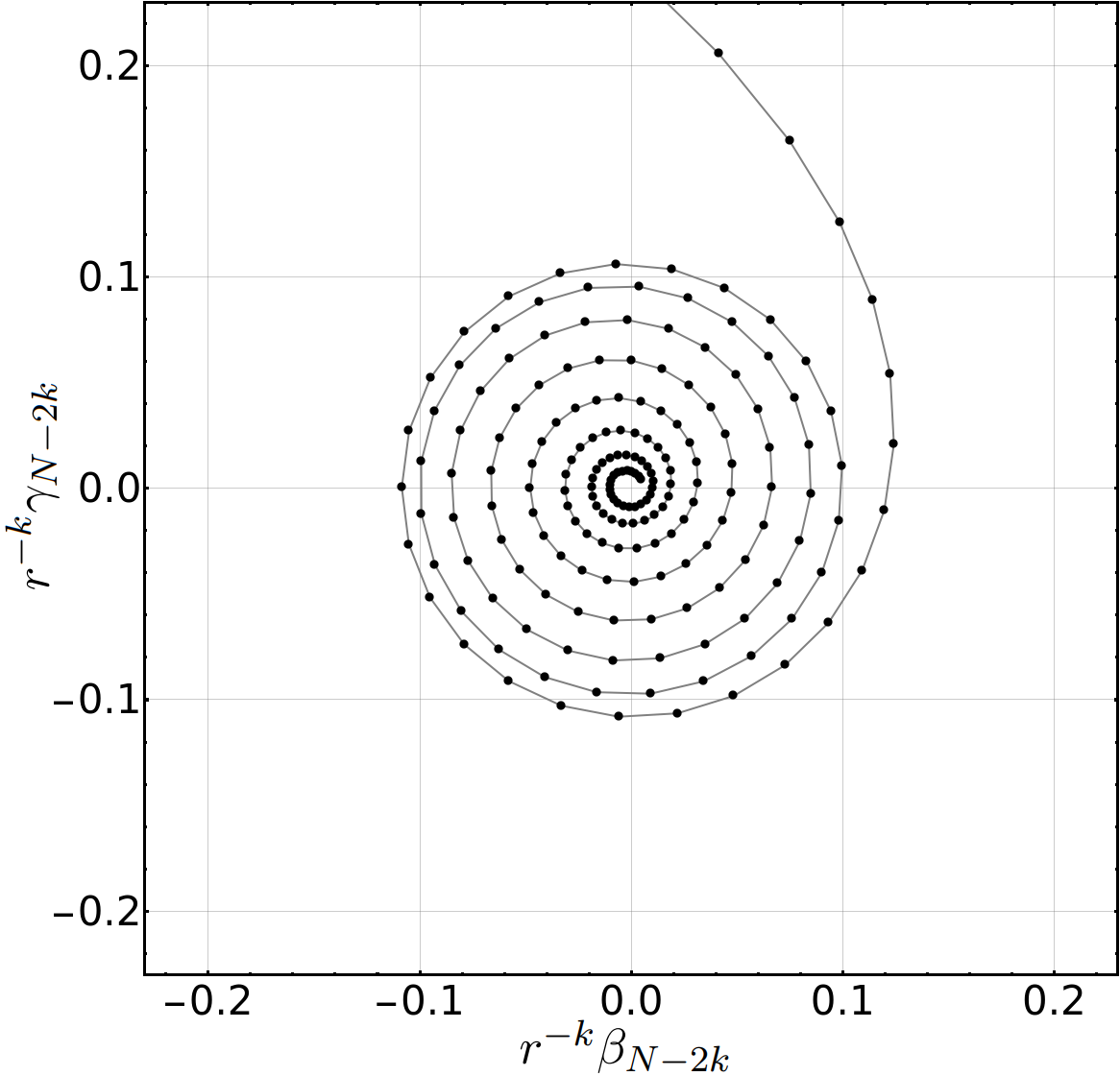
Figure 1: RG evolution of vector $\vec{\xi}(n)$ near the attractive nearly-fixed point $\vec{\xi}^{+}(n)$ for the running energy cutoff $n=N-2k$ and $k$ ranging from $8$ to $200$. Coordinates $\beta$ and $\gamma$ are defined in Eqs. (23b) and (23c) for ${\Delta\vec{\xi}(N-2k)=\vec{\xi}(N-2k)-\vec{\xi}^{+}(N-2k)}$. The initial cutoff is ${N=1000}$ and ${\vec{\xi}_{N}=\left(1,1,1\right)}$. The floating fixed point $\vec{\xi}^{+}(N-2k)$ is derived numerically by applying the exact RGT of Eqs. (5) to ${\vec{\xi}_{N^{\prime}}=\left(1,1,1\right)}$ with ${N^{\prime}=1200}$, while ${E=0}$ and ${g=1}$. The points do not lie on a circle, as they would in case of the approximate RGT of Eqs. (8), because the rate of spiral convergence per cycle in the exact RGT is slightly greater than $r^{t}$. The consecutive points are connected to guide the eye.

III.4 Variation of the RG spiral with floating cutoff $n$

It is pointed out at the end of previous subsection that the matrix $\vec{F}^{\prime}_{n}[\vec{\xi}^{+}(n)]$ in Eq. (36) depends on the floating cutoff $n$ so that the exact RGT produces a non-monotonous spiral flow in Fig. 1, instead of the circle that the simplified Eq. (33) would yield in terms of the coordinates $(\beta,\gamma)_{\rm scaling}$. This feature is a consequence of the fact that the moduli of eigenvalues of $\vec{F}^{\prime}_{n}[\vec{\xi}^{+}(n)]$ don’t have a constant value equal to $r$. The rate of spiral convergence per one RGT step is instead given by some $n$-dependent value $r_{n}$. For large $n$, $r_{n}$ is given by the same formulas as $r$ except that the fixed $N$ is replaced by the floating $n$,

$$r_{n}=\frac{1-p_{n}}{1+p_{n}}\ ,$$ (38)

where ${p_{n}^{2}=\sqrt{a_{n}+(a_{n}/2)^{2}}-a_{n}/2}$ and ${1/a_{n}=4gn}$. The convergence factor after $k$ RGT steps is thus given by

$$R(N,k)=r_{N-2}\cdot\dotsc\cdot r_{N-2k}\ ,$$ (39)

which replaces $r^{k}$. The difference between $r^{k}$ and varying convergence factors $R(N,k)$ is illustrated in the top panel of Fig. 2, where we plot points with coordinates

$$(\beta,\gamma)_{\rm scaling\ 1} = R(N,k)^{-1}\left(\beta_{N-2k},\gamma_{N-2k}\right)\ .$$ (40)

Distance of these points from ${\left(0,0\right)}$ is roughly constant for $\beta>0$ and $\gamma<0$, and it increases with increasing number of cycles for points lying in the first, second and third quadrants of the coordinate system.

Figure 2: The same RG spiral as in Fig. 1 displayed in terms of three different coordinate systems, from top to bottom: ${(\beta,\gamma)_{\rm scaling\ 1}}$ of Eq. (40), ${(\beta,\gamma)_{\rm scaling\ 2}}$ of Eq. (41) and ${(\beta,\gamma)_{\rm scaling\ 3}}$ of Eq. (42), correspondingly. Coordinates used in the top figure account for the cutoff flow of the spiral convergence rate $r$. The middle figure shows the effect of variation of the basis vectors formed by the eigenvectors of the RGT derivative near the floating fixed-point $\vec{\xi}^{+}(n)$. The bottom figure shows the result of simultaneous account for the both effects.

Variation with $n$ of the eigenvectors $\vec{v}$, $\vec{v}_{1}$ and $\vec{v}_{2}$ of the derivative $\vec{F}^{\prime}_{n}[\vec{\xi}^{+}(n)]$ is illustrated in the middle panel of Fig. 2. One changes the coordinates $\alpha$, $\beta$, $\gamma$ correspondingly to the replacement of $p$ by $p_{n}$ in Eqs. (23). The new coordinates are denoted by $\tilde{\alpha}_{n}$, $\tilde{\beta}_{n}$, $\tilde{\gamma}_{n}$. The middle panel of Fig. 2 shows the RG flow of

$$(\beta,\gamma)_{\rm scaling\ 2} = r^{-k}\left(\tilde{\beta}_{N-2k},\tilde{\gamma}_{N-2k}\right)\ .$$ (41)

In this representation the spiral converges quite uniformly, as opposed to the somewhat erratic convergence illustrated in Fig. 1, where one uses the fixed basis of Eqs. (23).

The bottom panel in Fig. 3 displays the flow of $\Delta\vec{\xi}$ using coordinates

$$(\beta,\gamma)_{\rm scaling\ 3} = R(N,k)^{-1}\left(\tilde{\beta}_{N-2k},\tilde{\gamma}_{N-2k}\right)\ .$$ (42)

Somewhat erratic spiral flow in Fig. 1, the angular asymmetry visible in the top panel of Fig. 2, the regular spiral in the middle panel of Fig. 2 and the circle shown in the bottom panel of Fig. 2 together identify and summarize the main features of the RG spiral flow of the quartic oscillator Hamiltonian with the cutoff near the attractive sequence $\vec{\xi}^{+}(n)$. When the dependence of eigenvalues and eigenvectors of the derivative $\vec{F}^{\prime}_{n}[\vec{\xi}^{+}(n)]$ is factored out, the scaling $\Delta\vec{\xi}(n)$ moves around a circle. The remaining apparent variation of the circle radius is not further discussed in this paper.

III.5 Repulsive floating fixed-point $\vec{\xi}^{-}(n)$

The approximate RGT has a second fixed point solution $\vec{\xi}^{-}$ defined in Eq. (12b). The corresponding eigenvalues of the derivative matrix $\vec{F}^{\prime}[\vec{\xi}^{-}]$ are $r^{-1}$, $r^{-1}e^{i\omega}$, $r^{-1}e^{-i\omega}$, with the same $r$ and $\omega$ as for $\vec{\xi}^{+}$. This implies that $\vec{\xi}^{-}$ is a repulsive fixed point. The sequences of $\vec{\xi}$ that start in the vicinity of $\vec{\xi}^{-}$, move away from $\vec{\xi}^{-}$ following a spiral curve. The rate of divergence per step is $r^{-1}$, which is an inverse of the rate of convergence on $\vec{\xi}^{+}$. The frequency with which the spiral unfolds around $\vec{\xi}^{-}$ is $\omega$, the same as in the case of folding in around $\vec{\xi}^{+}$.

Similarly to the attractive fixed point, the repulsive fixed point $\vec{\xi}^{-}$ of the approximate RGT has a counterpart in the exact RGT, which is a repulsive floating fixed-point $\vec{\xi}^{-}(n)$. The sequences repelled from $\vec{\xi}^{-}(n)$ can be equivalently described as the convergent sequences that are generated by the inverse RGT,

$$\xi_{1}(n)=-\frac{n-E}{g\phi(n)}+\frac{\phi_{2}(n)}{1-\xi_{2}(n-2)},$$ (43a)

$$\xi_{2}(n)=\xi_{1}(n-2)+\frac{\phi_{1}(n)\phi_{2}(n)}{\phi_{3}^{2}(n)}\frac{\left[1-\xi_{3}(n-2)\right]^{2}}{1-\xi_{2}(n-2)},$$ (43b)

$$\xi_{3}(n)=\frac{\phi_{2}(n)}{\phi_{3}(n)}\frac{1-\xi_{3}(n-2)}{1-\xi_{2}(n-2)}.$$ (43c)

These sequences converge to $\vec{\xi}^{-}(n)$. The inverse RGT can be used to find numerical approximations for the repulsive floating fixed-point sequence.

One might expect that the sequence $\vec{\xi}(n)$ that is repelled from $\vec{\xi}^{-}(n)$ goes over to the attractive sequence $\vec{\xi}^{+}(n)$. However, the sequences generated by the RGT from the initial conditions $\vec{\xi}(N)$ in the vicinity of the repulsive fixed point, do not always simply transit over to the attractive fixed point as it is the case for the initial condition ${\vec{\xi}(N)=(1,1,1)}$. We illustrate this finding in Fig. 3, where plots of the projection

$$f(k)=\left[\vec{\xi}(N-2k)-\vec{\xi}^{-}\right]\cdot\frac{\vec{\xi}^{+}-\vec{\xi}^{-}}{\left(\vec{\xi}^{+}-\vec{\xi}^{-}\right)^{2}}\ ,$$ (44)

as a function of the number of RGT steps $k$, are shown for three different initial points $\vec{\xi}(N)$.

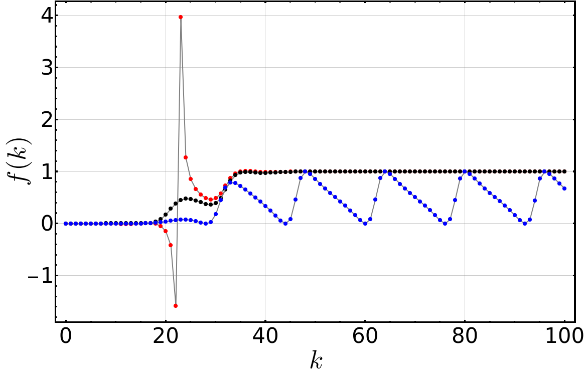
Figure 3: Examples of sequences of projections $f(k)$ of Eq. (44), where $k$ is the number of RGT steps. Value ${f(k)=0}$ corresponds to projection of $\vec{\xi}(N-2k)$ being the same as for $\vec{\xi}^{-}$ and ${f(k)=1}$ means that the projection of $\vec{\xi}(N-2k)$ is the same as for $\vec{\xi}^{+}$. The points are generated by the approximate RGT with $6gN=10^{3}$ and initial conditions $\vec{\xi}(N)=\vec{\xi}^{-}+(10^{-6},10^{-6},10^{-6})$ (black points), $\vec{\xi}(N)=\vec{\xi}^{-}+(10^{-6},10^{-6},2\times 10^{-6})$ (red points) and $\vec{\xi}(N)=\vec{\xi}^{-}+(10^{-6},10^{-6},1.5\times 10^{-6})$ (blue points). The points are connected to guide the eye.

The first sequence, represented by the black dots, approaches 1, which corresponds to ${\vec{\xi}(N-2k)=\vec{\xi}^{+}}$, after just two turns. The second sequence, represented by the red points, makes a relatively big jump before reaching 1, which is caused by the approximate RGT denominator $d_{s}(n)={\xi_{1}(n)+1/(6gN)}$ in Eq. (9) becoming negative for some value of $n$ just before the jump. The third sequence, represented by the blue points, doesn’t converge to 1 at all.

The effects displayed in Fig. 3 are due to a special property of the simplified RGT of Eqs. (8). Namely, any two sequences generated by the approximate RGT, say $\vec{\xi}_{A}(n)$ and $\vec{\xi}_{B}(n)$, satisfy the equation

$$h\left[\vec{\xi}_{A}(n-2)-\vec{\xi}_{B}(n-2)\right]=$$

$$=\frac{h\left[\vec{\xi}_{A}(n)-\vec{\xi}_{B}(n)\right]}{36\left[\xi_{A1}(n)+1/(6gN)\right]\left[\xi_{B1}(n)+1/(6gN)\right]}\ ,$$ (45)

where ${h\left[\vec{v}\right]=v_{1}v_{2}-(4/9)v_{3}^{2}}$. Equation ${h\left[\vec{\xi}-\vec{\xi}^{-}\right]=0}$ describes a cone in the three-dimensional space of $\vec{\xi}$. The tip of the cone is in ${\vec{\xi}=\vec{\xi}^{-}}$. If an initial condition $\vec{\xi}(N)$ lies on that cone, that is if ${h\left[\vec{\xi}(N)-\vec{\xi}^{-}\right]=0}$, then according to Eq. (III.5) with ${\vec{\xi}_{A}(n)=\vec{\xi}(n)}$ and ${\vec{\xi}_{B}(n)=\vec{\xi}^{-}}$, all terms of the sequence $\vec{\xi}(n)$, generated by the simplified RGT of Eq. (8), lie on the same cone, that is $h\left[\vec{\xi}(n)-\vec{\xi}^{-}\right]=0$ for ${n=N-2,N-4,N-6}$ and so on. Hence, $\vec{\xi}(n)$ cannot reach $\vec{\xi}^{+}$ no matter how close to 1 its projection $f(k)$ gets. For the attractive point $\vec{\xi}^{+}$ does not lie on the same cone. An example of the RG flow that keeps cyclically coming close to $\vec{\xi}^{+}$ but always misses it, is shown by the blue points in Fig. 3.

Furthermore, since the attractive fixed point lies inside the cone, for $h\left[\vec{\xi}^{+}-\vec{\xi}^{-}\right]>0$, the sequences that start from an initial condition $\vec{\xi}(N)$ outside the cone and eventually converge on $\vec{\xi}^{+}$, so that initially $h\left[\vec{\xi}(N)-\vec{\xi}^{-}\right]<0$ and eventually $h\left[\vec{\xi}(n)-\vec{\xi}^{-}\right]>0$, must make a similar jump to the one made by the sequence represented by the red points in Fig. 3. They have to make the jump because the sequence $h\left[\vec{\xi}(n)-\vec{\xi}^{-}\right]$ must change its sign from negative to positive for some value of the floating cutoff $n_{0}$,

$$h\left[\vec{\xi}(n_{0})-\vec{\xi}^{-}\right]<0\ ,$$ (46a)

$$h\left[\vec{\xi}(n_{0}-2)-\vec{\xi}^{-}\right]>0\ .$$ (46b)

According to Eq. (III.5), this can only happen if ${\xi_{1}(n_{0})+1/(6gN)<0}$.

Analogous condition to Eq. (III.5) holds for the exact RGT,

$$h\left[\vec{\xi}_{A}(n-2)-\vec{\xi}_{B}(n-2),n-2\right]=$$

$$=\frac{\phi_{2}(n)\,h\left[\vec{\xi}_{A}(n)-\vec{\xi}_{B}(n),n\right]}{\left(\xi_{A1}(n)+\frac{n-E}{g\phi(n)}\right)\left(\xi_{B1}(n)+\frac{n-E}{g\phi(n)}\right)}\ ,$$ (47)

where $h\left[\vec{v},n\right]=v_{1}v_{2}-\phi_{1}(n)v_{3}^{2}$, which explains the exceptions mentioned in Sec. III.3; that there exist sequences that do not converge on $\vec{\xi}^{+}(n)$ even if they come close.

Projection $f(k)$ can also be defined by replacing $\vec{\xi}^{+}$ and $\vec{\xi}^{-}$ in Eq. (44) with the floating fixed points $\vec{\xi}^{+}(N-2k)$ and $\vec{\xi}^{-}(N-2k)$. One can derive the approximate values of $\vec{\xi}^{+}(N-2k)$ and $\vec{\xi}^{-}(N-2k)$ numerically as described before and then generate plots of $f(k)$. Such plots are similar to those presented in Fig. 3. In particular, an oscillating sequence $f(k)$ analogous to the one represented by the blue points in Fig. 3, is generated for an initial condition $\vec{\xi}(N)$ satisfying ${h\left[\vec{\xi}(N)-\vec{\xi}^{-}(N),N\right]=0}$, while a sequence with a big jump analogous to the one represented by the red points can be obtained for an initial condition satisfying ${h\left[\vec{\xi}(N)-\vec{\xi}^{-}(N),N\right]<0}$.

IV Extension of the RG analysis

Our discussion of the quartic Hamiltonian RG behavior can be naturally extended in different ways described in this section.

IV.1 Polynomial interactions

The first type of extension concerns Hamiltonians of the form

$$H=-\frac{d^{2}}{d\varphi^{2}}+\sum_{i=2}^{M}A_{i}\,\varphi^{i}\ ,$$ (48)

where ${M>4}$ is a finite even number. $A_{M}$ is assumed positive for the energy spectrum to be bounded from below. $A_{2}$ is also assumed positive for the eigenstates of quadratic-oscillator Hamiltonian ${H_{0}=-d^{2}/d\varphi^{2}+A_{2}\,\varphi^{2}}$ to provide the basis in which one computes the Hamiltonian matrix $H^{\infty}_{k,l}$.

The RGT of the resulting matrix $H^{\infty}_{k,l}$ depends on the form of polynomial with ${i>2}$ in Eq. (48), which we call the interaction. If the interaction is even, that is if ${A_{i}=0}$ for odd $i$, then $H$ doesn’t mix even and odd eigenstates of $H_{0}$ and the number of bands of $H^{\infty}_{k,l}$ equals ${M+1}$. This implies that the cutoff flow of the Hamiltonian can be parameterized by a vector $\vec{\xi}(n)$ of dimension ${M(M/2+1)/4}$, defined analogously to the 3-dimensional case in Eqs. (4). If the potential is not even, then the number of bands equals ${2M+1}$ and the RGT acts on a ${M(M+1)/2}$-dimensional vector $\vec{\xi}(n)$. The RGT equation has a form ${\vec{\xi}(n-2)=\vec{F}[\vec{\xi}(n)]}$ in the case of even interactions and ${\vec{\xi}(n-1)=\vec{F}[\vec{\xi}(n)]}$ for the interactions that are not even. In the latter case the Gaussian elimination does not integrate out the even rows and columns of effective Hamiltonian independently from the odd ones. Vector $\vec{F}[\vec{\xi}]$ is a rational function of components of $\vec{\xi}$ and depends on $M$, ${A_{2},\dots,A_{M}}$, floating cutoff $n$ and energy $E$. One can study properties of the RGTs for band-diagonal Hamiltonians of Eq. (48) following the steps analogous to the case of ${M=4}$ discussed in the previous sections.

We illustrate complexity of the resulting RGTs using the case of ${M=6}$,

$$H=a^{\dagger}a+g\left(a+a^{\dagger}\right)^{6}\ .$$ (49)

The diagonal matrix elements of this Hamiltonian in the oscillator basis are

$$H_{n;n,n}^{N}=n+\xi_{1}(n)\left(H^{N}_{n,n}-n\right),$$ (50a)

$$H_{n;n-2,n-2}^{N}=n-2+\xi_{2}(n)\left[H^{N}_{n-2,n-2}-\left(n-2\right)\right],$$ (50b)

$$H_{n;n-4,n-4}^{N}=n-4+\xi_{3}(n)\left[H^{N}_{n-4,n-4}-\left(n-4\right)\right],$$ (50c)

and the off-diagonal ones are

$$H_{n;n,n-2}^{N}=H_{n;n-2,n}^{N}=\xi_{4}(n)H^{N}_{n,n-2},$$ (51a)

$$H_{n;n,n-4}^{N}=H_{n;n-4,n}^{N}=\xi_{5}(n)H^{N}_{n,n-4},$$ (51b)

$$H_{n;n-2,n-4}^{N}=H_{n;n-4,n-2}^{N}=\xi_{6}(n)H^{N}_{n-2,n-4}.$$ (51c)

The dimension of $\vec{\xi}(n)$ is 6, instead of 4 in Eqs. (4), because the matrix of Hamiltonian in Eq. (49) has more bands than the quartic-oscillator matrix. The RGT expressed in terms of $\vec{\xi}(n)$ is quite complex and we do not produce it here. In the limit of large floating cutoffs $n$ and the number of RGT steps ${(N-n)/2}$ much smaller than $N$, with all terms of order ${O\left(1/N^{3}\right)}$ dropped and using

$$d_{6}(n,N) = \xi_{1}(n)+1/(20gN^{2})\ ,$$ (52)

the RGT reads

$$\xi_{1}(n-2)=\xi_{2}(n)-\left(\frac{9}{16}+\frac{63}{64N^{2}}\right)\frac{\xi_{4}(n)^{2}}{d_{6}(n,N)}\ ,$$ (53a)

$$\xi_{2}(n-2)=\xi_{3}(n)-\left(\frac{9}{100}+\frac{63}{100N^{2}}\right)\frac{\xi_{5}(n)^{2}}{d_{6}(n,N)}\ ,$$ (53b)

$$\xi_{3}(n-2)=1-\left(\frac{1}{400}+\frac{63}{1600N^{2}}\right)\frac{1}{d_{6}(n,N)}\ ,$$ (53c)

$$\xi_{4}(n-2)=\xi_{6}(n)-\left(\frac{3}{10}+\frac{21}{20N^{2}}\right)\frac{\xi_{4}(n)\xi_{5}(n)}{d_{6}(n,N)}\ ,$$ (53d)

$$\xi_{5}(n-2)=1-\left(\frac{1}{8}+\frac{21}{32N^{2}}\right)\frac{\xi_{4}(n)}{d_{6}(n,N)}\ ,$$ (53e)

$$\xi_{6}(n-2)=1-\left(\frac{1}{50}+\frac{21}{100N^{2}}\right)\frac{\xi_{5}(n)}{d_{6}(n,N)}\ .$$ (53f)

The number of floating fixed-points of this RGT and their repulsive or attractive nature requires studies beyond what authors have done so far. In the limit ${n\sim N\to\infty}$ one can proceed in a simplified way, analogous to Secs. III.1 and III.2. The fixed points ${\vec{\xi}(n)=\vec{\xi}^{*}}$ of the RGTs in that limit can be derived numerically. For all values of $N$ and $g$ that we checked, ranging from ${N=1000}$ to ${N=10000}$ and from ${g=0.1}$ to ${g=10}$, the RGT possess 4 fixed points. One fixed point is attractive, one is repulsive and two other ones are mixed. In the latter, the derivative matrix $\vec{F}^{\prime}[\vec{\xi}^{*}]$ has some eigenvalues with modulus bigger than 1 and some with modulus smaller than 1, corresponding to Wegner’s relevant and irrelevant interaction terms [13].

IV.2 Quartic Hamiltonians with negative
coefficient $A_{2}$

The second case of interest concerns even Hamiltonians of the form displayed in Eq. (48) with ${M=4}$ and a negative coefficient $A_{2}$. It is naturally of interest because of the spontaneous breaking of $Z_{2}$ symmetry. Without losing generality, the Hamiltonian can be written in the form

$$H=a^{\dagger}a+g\left(a+a^{\dagger}\right)^{3}+g^{2}\left(a+a^{\dagger}\right)^{4}\ .$$ (54)

This form is derived by writing the quartic-oscillator Hamiltonian with negative quadratic coefficient,

$$H=-\frac{d^{2}}{d\varphi^{2}}-A\,\varphi^{2}+B\,\varphi^{4}\ ,$$ (55)

in terms of variable ${\phi=\varphi-\langle\varphi\rangle}$, which describes the deviation of $\varphi$ from one of its so-called vacuum expectation values ${\langle\varphi\rangle=\pm\sqrt{A/(2B)}}$. One rescales ${H\rightarrow H/(2\sqrt{2A})}$, introduces creation and annihilation operators via ${\phi=(8A)^{-1/4}\left(a+a^{\dagger}\right)}$, ${d/d\phi=(A/2)^{1/4}\left(a-a^{\dagger}\right)}$ and drops the constant term. The result of Eq. (54) follows with ${g=\sqrt{B}/\left(8A\right)^{3/4}}$.

The RGT for matrices of Hamiltonians obtained from Eq. (54) is described using a 10-dimensional vector $\vec{\xi}(n)$. The diagonal matrix elements are described by $\xi_{i}$ with $i=1,2,...,4$

$$H_{n;n,n}^{N}=n+\xi_{1}(n)\left(H^{N}_{n,n}-n\right),$$ (56a)

$$H_{n;n-1,n-1}^{N}=n-1+\xi_{2}(n)\left[H^{N}_{n-1,n-1}-\left(n-1\right)\right],$$ (56b)

$$H_{n;n-2,n-2}^{N}=n-2+\xi_{3}(n)\left[H^{N}_{n-2,n-2}-\left(n-2\right)\right],$$ (56c)

$$H_{n;n-3,n-3}^{N}=n-3+\xi_{4}(n)\left[H^{N}_{n-3,n-3}-\left(n-3\right)\right],$$ (56d)

and the off-diagonal terms by $\xi_{i}$ with $i=5,6,...,10$.

$$H_{n;n,n-1}^{N}=H_{n;n-1,n}^{N}=\xi_{5}(n)H^{N}_{n,n-1},$$ (57a)

$$H_{n;n,n-2}^{N}=H_{n;n-2,n}^{N}=\xi_{6}(n)H^{N}_{n,n-2},$$ (57b)

$$H_{n;n,n-3}^{N}=H_{n;n-3,n}^{N}=\xi_{7}(n)H^{N}_{n,n-3},$$ (57c)

$$H_{n;n-1,n-2}^{N}=H_{n;n-2,n-1}^{N}=\xi_{8}(n)H^{N}_{n-1,n-2},$$ (57d)

$$H_{n;n-1,n-3}^{N}=H_{n;n-3,n-1}^{N}=\xi_{9}(n)H^{N}_{n-1,n-3},$$ (57e)

$$H_{n;n-2,n-3}^{N}=H_{n;n-3,n-2}^{N}=\xi_{10}(n)H^{N}_{n-2,n-3}.$$ (57f)

As before, $H^{N}_{k,l}$ denote matrix elements of $H$. For $n\sim N\to\infty$ and using

$$d_{10}(n,N)=\xi_{1}(n)+1/(6g^{2}N)\ ,$$ (58)

the RGT is obtained in the simplified form in which all terms of order ${O\left(1/N^{2}\right)}$ are dropped.

$$\xi_{1}(n-1)=\xi_{2}(n)-\frac{1}{4g^{2}N}\frac{\xi_{5}(n)^{2}}{d_{10}(n,N)}\ ,$$ (59a)

$$\xi_{2}(n-1)=\xi_{3}(n)-\frac{4}{9}\frac{\xi_{6}(n)^{2}}{d_{10}(n,N)}\ ,$$ (59b)

$$\xi_{3}(n-1)=\xi_{4}(n)-\frac{1}{36g^{2}N}\frac{\xi_{7}(n)^{2}}{d_{10}(n,N)}\ ,$$ (59c)

$$\xi_{4}(n-1)=1-\frac{1}{36}\frac{1}{d_{10}(n,N)}\ ,$$ (59d)

$$\xi_{5}(n-1)=\xi_{8}(n)-\left(\frac{2}{3}-\frac{1}{3N}\right)\frac{\xi_{5}(n)\xi_{6}(n)}{d_{10}(n,N)}\ ,$$ (59e)

$$\xi_{6}(n-1)=\xi_{9}(n)-\frac{1}{8g^{2}N}\frac{\xi_{5}(n)\xi_{7}(n)}{d_{10}(n,N)}\ ,$$ (59f)

$$\xi_{7}(n-1)=1-\left(\frac{1}{2}-\frac{1}{2N}\right)\frac{\xi_{5}(n)}{d_{10}(n,N)}\ ,$$ (59g)

$$\xi_{8}(n-1)=\xi_{10}(n)-\left(\frac{2}{9}-\frac{1}{9N}\right)\frac{\xi_{6}(n)\xi_{7}(n)}{d_{10}(n,N)}\ ,$$ (59h)

$$\xi_{9}(n-1)=1-\frac{1}{6}\frac{\xi_{6}(n)}{d_{10}(n,N)}\ ,$$ (59i)

$$\xi_{10}(n-1)=1-\left(\frac{1}{18}-\frac{1}{18N}\right)\frac{\xi_{7}(n)}{d_{10}(n,N)}\ .$$ (59j)

The evolution of the 10-dimensional vector $\vec{\xi}(n)$ exhibits similar features to the ones described at the end of Sec. IV.1. However, the case of 10 dimensions is much richer in structure and more difficult to fully analyze. The authors have not completed the full analysis.

IV.3 Extension to quantum field theory

The third way of extending our RG analysis of just one quartic oscillator concerns two or more oscillators that interact with each other. In particular, denoting one such oscillator variable by $\varphi_{1}$ and another one by $\varphi_{2}$, one can consider interactions of the form $(\varphi_{1}-\varphi_{2})^{2}/(2a^{2})$. The parameter $a$ corresponds to a discrete approximation for the spatial derivative $d\varphi/dx$ with $dx$ replaced by $a$. Including more oscillators and labeling them by vectors $\vec{m}=(m_{1},m_{2},m_{3})$ with integer components, one can think about the oscillator variable $\varphi_{\vec{m}}$ as a quantum field at a space grid point $\vec{x}=a\vec{m}$. The new element of such setup for studying scalar theory on the spacial lattice is that the oscillators at each and every point $\vec{x}$ are cut off in ultraviolet by a cutoff $N$ and involve a corresponding vector $\vec{\xi}(\vec{x},N)$.

Consider the Hamiltonian for two oscillators $\varphi_{1}$ and $\varphi_{2}$ coupled by the term

$$(\varphi_{1}-\varphi_{2})^{2}/(2a^{2})=\varphi_{1}^{2}/(2a^{2})+\varphi_{2}^{2}/(2a^{2})-\varphi_{1}\varphi_{2}/a^{2}\ .$$ (60)

The first two terms on the right-hand side individually modify the quadratic terms of each of the oscillators. The only term that couples the oscillators is the third one. It is capable of exciting or de-exciting both oscillators by 1, or exciting one oscillator by 1 and de-exciting the other one by 1. The interaction contributes to the matrix elements of the Hamiltonian, denoted in a self-explanatory way by $H^{N}_{k_{1},k_{2};l_{1},l_{2}}$. The matrix elements involve two 3-dimensional vectors $\vec{\xi}(1,N)$ and $\vec{\xi}(2,N)$. However, the number of eigenstates of definite free oscillator energy $K$ in units of the modified $\hbar\omega$ is $K+1$. The Gaussian elimination becomes complicated. The authors have not identified any simple way to carry it out. The RG analysis of a similar Hamiltonian matrix for an entire grid of oscillators not only involves the vector $\vec{\xi}(N)$ as many times as there are grid points but also must deal with a significant increase in degeneracy. Implications of setting up a regulated quantum field theory this way, with finite parameters $N$ and $a$, require investigation, including the issue of how to approach the limits of $N\to\infty$ and ${a\to 0}$ simultaneously.

V Conclusion and outlook

This article establishes that the basic quantum-physics system of an oscillator with a quartic interaction term, exhibits the spiral cutoff dependence in the Wilsonian renormalization group procedure. Its Hamiltonian matrix in the basis of harmonic oscillator eigenstates is band-diagonal and its cutoff flow involves only the several matrix elements between the basis states of highest allowed oscillator energy. These evolving matrix elements are parameterized in terms of components of the 3-dimensional vector that spirals towards a slowly drifting, attractive fixed point as the cutoff decreases, with some exceptions.

Renormalization of band-diagonal Hamiltonian matrices was discussed in the past, see e.g. [[SeeApp.Bin]GW93]. However, to the best of authors’ knowledge the possibility of a cutoff spiral flow in them was not noted to exist. Such possibility is also difficult to note in case of the quartic oscillator, because the initial spiral contraction rate can be so large that it causes an illusion of a rapid convergence to an apparent fixed point.

Further renormalization-group studies of polynomial interactions are worth pursuing for the purpose of understanding their cutoff dependence, see Sec. IV. In particular, studies of polynomial interactions of order 4 with negative quadratic term are desired for understanding the dynamics of spontaneous breaking of $Z_{2}$ symmetry. Generalization of the RG studies to coupled quartic oscillators provides a way to investigate the role of cutoffs in Hamiltonian formulation of quantum field theory.

It should be stressed that this paper does not discuss corrections due to the energy eigenvalues $E$ that enter the Gaussian elimination. An example that illustrates a method for analyzing such dependence using expansion in powers of the ratio $E/n$, where $n$ stands for the floating cutoff, is available in [12].

Acknowledgement

The authors thank Kamil Serafin for his suggestion that one could consider a slowly varying point, instead of a fixed one, to describe results obtained in Ref. [6].

References

- Bender and Wu [1969] C. M. Bender and T. T. Wu, Anharmonic Oscillator, Phys. Rev. 184, 1231 (1969).
- Workman et al. [2022] R. L. Workman et al. (Particle Data Group), Review of Particle Physics, Prog. Theor. Exp. Phys. 2022, 083C01 (2022).
- Chan et al. [1964] S. I. Chan, D. Stelman, and L. E. Thompson, Quartic Oscillator as a Basis for Energy Level Calculations of Some Anharmonic Oscillators, The Journal of Chemical Physics 41, 2828 (1964).
- Wilson [1983] K. G. Wilson, The renormalization group and critical phenomena, Rev. Mod. Phys. 55, 583 (1983).
- Lyth and Riotto [1999] D. H. Lyth and A. Riotto, Particle physics models of inflation and the cosmological density perturbation, Physics Reports 314, 1 (1999).
- Wójcik [2013] K. Wójcik, Application of a Numerical Renormalization Group Procedure to an Elementary Anharmonic Oscillator, Acta Phys. Polon. B 44, 69 (2013).
- Wilson [1965] K. G. Wilson, Model Hamiltonians for Local Quantum Field Theory, Phys. Rev. 140, B445 (1965).
- Wilson [1970] K. G. Wilson, Model of Coupling-Constant Renormalization, Phys. Rev. D 2, 1438 (1970).
- Weinberg [1995] S. Weinberg, The Quantum Theory of Fields, Vol. 1 (Cambridge University Press, 1995).
- Wilson et al. [1994] K. G. Wilson, T. S. Walhout, A. Harindranath, W.-M. Zhang, R. J. Perry, and S. D. Głazek, Nonperturbative QCD: A weak-coupling treatment on the light front, Phys. Rev. D 49, 6720 (1994).
- Wilson [1971] K. G. Wilson, Renormalization Group and Strong Interactions, Phys. Rev. D 3, 1818 (1971).
- Głazek and Wilson [2004] S. D. Głazek and K. G. Wilson, Universality, marginal operators, and limit cycles, Phys. Rev. B 69, 094304 (2004).
- Wegner [1972] F. J. Wegner, Corrections to Scaling Laws, Phys. Rev. B 5, 4529 (1972).
- Głazek and Wilson [1993] S. D. Głazek and K. G. Wilson, Renormalization of Hamiltonians, Phys. Rev. D 48, 5863 (1993).
- Weniger [1996] E. J. Weniger, Construction of the Strong Coupling Expansion for the Ground State Energy of the Quartic, Sextic, and Octic Anharmonic Oscillator via a Renormalized Strong Coupling Expansion, Phys. Rev. Lett. 77, 2859 (1996).