Classical echoes of quantum boundary conditions
Abstract
We consider a non-relativistic particle in a one-dimensional box with all possible quantum boundary conditions that make the kinetic-energy operator self-adjoint. We determine the Wigner functions of the corresponding eigenfunctions and analyze in detail their classical limit in the high-energy regime. We show that the quantum boundary conditions split into two classes: all local and regular boundary conditions collapse to the same classical boundary condition, while singular non-local boundary conditions slightly persist in the classical limit.
Keywords: Classical limit, Wigner function, Particle in a box, Quantum boundary conditions, Self-adjoint extensions
1 Introduction
The phase-space formulation of quantum mechanics allows to represent states and operators as functions on classical phase-space [1]. It has various applications, ranging from quantum optics, quantum chaos and quantum computing to classical optics and signal analysis [2, 3]. In quantum physics, phase-space methods have also been used to characterize the non-classicality of quantum states, to identify and reconstruct states via quantum tomography, and to understand the quantum-to-classical transition and the correspondence principle [4, 5, 6, 7].
Between many possible quantum (quasi-)probability distributions, the Wigner function arguably gives the most natural phase-space representation of quantum mechanics. In spite of a long history of research, the theory of Wigner functions for systems on a manifold (or phase-space) with non-trivial topology, as well as having boundaries, is still not complete. For example, group-theoretical approaches have recently been applied for the Wigner function on the cylinder [8, 9], the discrete cylinder [10, 11] and the torus [12], whereas the deformation quantization approach is usually employed for manifold with boundaries, see e.g. [13, 14, 15, 16].
In this paper, we are interested in two related subjects: (i) the study of the Wigner function for eigenfunctions of the kinetic-energy operator (i.e. the free Hamiltonian) acting in a one-dimensional box with general self-adjoint boundary conditions, and (ii) the analysis of these Wigner functions in the classical limit, that is in the high-energy regime. Preliminary results in this direction have already been obtained: the Wigner function has been studied in [17, 18] for the one-dimensional box with Dirichlet boundary conditions, and in [19, 20] for the half-line with Robin boundary conditions. Besides, in [21, 22, 23] the classical limit of the position and momentum probability distributions for the one-dimensional box with Dirichlet boundary conditions have been investigated.
The paper is organized as follows. After introducing in Sec. 2 the free Hamiltonian with general self-adjoint boundary conditions, in Sec. 3 we explicitly compute the Wigner functions associated with the eigenfunctions of the Hamiltonian, and describe how to determine their classical limit. In Sec. 4, then, we classify the possible classical limits by analyzing the asymptotic properties of the spectrum in the high-energy regime. Finally, in Sec. 5 we discuss the results and compare the classical limits with corresponding classical probability distributions.
2 A quantum particle in a box
We consider a quantum particle of mass , confined in a one-dimensional box of unit length, namely the interval . This system is formally described by the kinetic-energy operator, )
| (1) |
which acts on a proper subspace of the Hilbert space . As it is well-known, see e.g. [24, 25], Eq. (1) prescribes the action of only in the bulk of the system. The Hamiltonian should indeed be equipped with suitable boundary conditions (BCs), specifying the behavior of the particle at the boundary of the interval, in order to generate a well-defined quantum dynamics. In quantum mechanics the possible BCs, encoded in the domain of , cannot be arbitrary, but are constrained by the requirement that must be a self-adjoint operator, i.e. and . Indeed, self-adjointness is a necessary and sufficient condition for a (Hermitian) operator to have a purely real spectrum and to generate a unitary dynamics.
Different domains correspond to different behaviors of the particle at the boundary, give rise to different dynamics and represent different physical situations. All the self-adjoint realizations of the operator (1) are known to be in one-to-one correspondence with the set of unitary matrices [26, 27, 28, 29]. Each of these realizations, which we henceforth denote by , is defined on the domain
| (2) |
where is the space of wave functions with square-integrable first and second derivative, and , on the interval , whereas
| (3) |
is defined in terms of the following boundary values111In some related works, as e.g. [26, 27, 28], the alternative parametrization is adopted, with a given ; here, following [29, 31], we find convenient to put .
| (4) |
Let us now introduce the Wigner function associated with a wave function , [1, 2, 3, 30]. The Wigner function represents the joint quasi-probability distribution of position and momentum in the state and it is given by
| (5) |
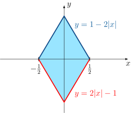
where . For a wave function spatially confined in the interval , i.e. for an element of , the associated Wigner function of can be computed considering the function defined on that coincides with in the interval and vanishes outside. With this procedure one obtains
| (6a) | ||||
| (6b) | ||||
where is the characteristic function of the interval , i.e. if and if , see Fig. 1. We stress that, although being defined for , by construction the above Wigner function vanishes for , i.e. outside of the box.222Interestingly, Eq. (6) can also be obtained by applying a “regularization” procedure: in [32], e.g., a particle moving freely on the half-line is treated as moving on the full line in the presence of an infinite potential wall, the latter being realized as a limit of a smooth (Morse) potential.
In the following we are interested both in the explicit expression of the Wigner function for an eigenfunction of , which will be the main topic of Sec. 3, and in its behavior in the classical limit, which we will discuss in Sec. 4. Before moving on, however, we spend a few words on the allowed quantum BCs, giving some examples in Sec. 2.1 and introducing a useful parametrization of in Sec. 2.2.
2.1 Topology of quantum boundary conditions
It is convenient to rewrite the boundary values in (4) as
| (7) |
so that, if the matrix is invertible, the BC in Eq. (3) can also be expressed as
| (8) |
where , being the inverse Cayley transform of , is an Hermitian matrix. For a more general inversion formula, holding also when is not invertible, see e.g. Eq. (19) of [31]. Two interesting families of BCs are given respectively by (symmetric) Robin conditions
| (9) |
with , that reduce to Dirichlet () and Neumann () BCs respectively for and , and by pseudo-periodic BCs
| (10) |
with , that in turn reduce to periodic and anti-periodic conditions when and , respectively.
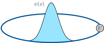
As the reader may have noticed, BCs can be either local or non-local: Robin BCs, e.g., are local, as they do not mix the boundary values of at the left edge with those at the right edge , whereas pseudo-periodic BCs are non-local. Differently from local BCs, which physically model a particle in a box, non-local BCs are actually related to the physics of a particle in a ring. Arbitrary BCs, thus, can be realized in a ring with a junction, the matrix encoding the physical properties of the latter, see Fig. 2. Note that this setup describes also local BCs, as the junction may eventually act as an impenetrable barrier that “decouples” the left edge from the right one.
More generally, let us stress that BCs are often crucial to determine the spatial topology of a quantum system, see e.g. [33, 26, 34, 35, 36, 37, 38, 39] for further details.
2.2 Parametrization of the quantum boundary conditions
All the unitary matrices in can be parametrized by using five real parameters [40]:
| (11) |
with , and such that
| (12) |
In order to obtain a one-to-one parametrization of , the values and have to be identified, as they give the same matrix:
| (13) |
To achieve this, we henceforth restrict . On the other hand, Eq. (12) tells us that only four parameters are actually independent and, since the pair always takes values in the unit disk , it is convenient to express and in terms of a new parameter :
| (14) |
Therefore we have that
| (15) |
where for all , and :
| (16) |
Notice that if then the matrix does not depend on , in that case we will fix .
Observe that Robin BCs (9) correspond to
| (17) |
whereas pseudo-periodic BCs (10) correspond to
| (18) |
The eigenvalues of depend only on and and are given by
| (19) |
and in particular
| (20a) | ||||
| (20b) | ||||
The above values are relevant since the inverse Cayley transform of is singular whenever is not invertible, that is when or is equal to . Otherwise, it is the well defined Hermitian matrix
| (21) |
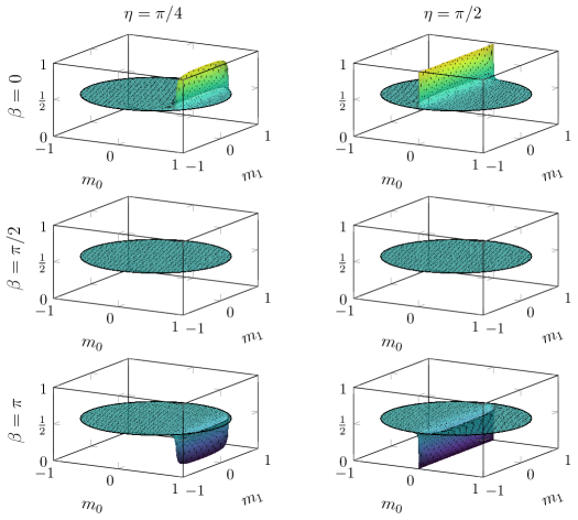
where . In Fig. 3, BCs having at least one eigenvalue equal to are represented in the parameter space of , for a given value of . Note that, in particular, the Dirichlet condition is the only one having .

For later convenience, we introduce the definition of regular and singular BCs. We say that the unitary matrix (and the corresponding BC) is singular if the eigenvalues satisfy and , that is if
| (22) |
while it is regular otherwise. In other words the matrices in having zero or two eigenvalues equal to are regular, while the ones having just one eigenvalue are singular. Besides, excluding the case of the identity matrix (corresponding to the Dirichlet condition), which is regular by definition but does not admit the inverse Cayley transform, a generic unitary matrix is regular if and only if it admits the inverse Cayley transform. Notice that the matrices corresponding to Robin BCs in Eq. (17) are regular (including the Dirichlet condition), while the matrices corresponding to pseudo-periodic BCs in Eq. (10) are singular.
3 Wigner functions
In this section we explicitly determine the Wigner function of an eigenfunction of , with , and , that is a non-zero solution of the eigenvalue equation
| (23) |
More in detail, after solving in Sec. 3.1 the spectral problem of , by determining its eigenfunctions in terms of the zeroes of a certain spectral function, in Sec. 3.2 we compute the corresponding Wigner functions, and analyze some of their properties in the high-energy regime. Then, in Sec. 3.3 we review the phase-space description of a classical particle in a box in order to compare the results.
3.1 Spectral problem
The eigenvalue equation (23) can be rewritten as the ordinary differential equation
| (24) |
further supplied by the BC in Eq. (3). Here, represents the dimensionless energy. For , the eigenvalue equation (24) has a general solution of the form
| (25) |
where , is a normalization constant, and
| (26) |
is the dimensionless wave number. Differently from which is always real, can be either real or purely imaginary, respectively when or . We recall that, in general, the eigenvalues of accumulate to and can be at most doubly degenerate (see e.g. Theorem 10.6.1 of [41]), thus depending on there can be at most two vanishing eigenvalues . Moreover, the sum of the multiplicities of the negative eigenvalues is at most two [25, 40].
To impose the BC in Eq. (3), after substituting Eq. (25) in the expression (4) of the boundary values , we rewrite the latter as
| (27) |
The BC can then be expressed as the homogeneous system
| (28) |
whose non-trivial solutions are obtained by requiring that
| (29) |
In other words, the non-vanishing eigenvalues of correspond to the real zeroes of the spectral function .333We mention that the definition of the spectral function can be modified to account also for the zero eigenvalues, see [40] for details. In terms of the parametrization (16), it is known [25, 27, 40] that, for ,
| (30) |
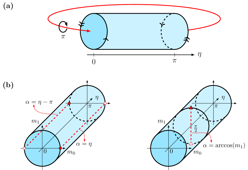
with as in Eq. (26). As it turns out, the spectrum depends only on three of the four independent parameters characterizing the matrix . Namely, it depends on , and , which by now we call spectral parameters, but not on , the non-spectral parameter. Seen as a manifold, the spectral space
| (31) |
has the same structure of a (twisted) solid torus [40], see Fig. 4 (a). In Fig. 4 (b), as an example, we represent in both Robin and pseudo-periodic conditions.
The zeroes of can be found analytically only for some particular BCs. Nevertheless, as we will show, their asymptotic behavior in the high-energy regime follows a simple pattern. Since we are interested in the classical limit, that is in the high-energy regime, from now on we will focus only on the positive part of the spectrum:
| (32) |
For the time being, let us denote with
| (33) |
the sequence of the positive zeroes of and with
| (34) |
the corresponding wave numbers, so that we have
| (35) |
To fix the expression of the eigenfunctions, we need to explicitly determine the coefficients and the normalization . By using Eq. (28) we find
| (36) | ||||
| (37) |
where and as in Eq. (14). The above expressions reveal that, differently from the spectrum, the coefficients of the eigenfunctions in Eq. (25) do actually depend on the non-spectral parameter . In conclusion, the function
| (38) |
where and , is a normalized eigenfunction of corresponding to the eigenvalue . For later convenience let us observe that, in the expression (37) for the normalization , the interference term proportional to is negligible for large , thus we have
| (39) |
3.2 Classical limit of the Wigner functions
At this point we are ready to compute the Wigner function associated with an eigenfunction (3.1). Using the definition in Eq. (6) we obtain
| (40) |
where for each :
| (41) |
with the triangular envelope and the sinc functions being respectively given by
| (42) |
A plot of is given in Fig. 5.
The classical limit can be implemented by taking , so that is kept fixed [4, 5, 6, 42, 43, 44]. Formally, it is obtained by setting
| (43) |
where is a reference value of the classical momentum, related to the classical reference energy via
| (44) |
and by letting .
By plugging Eq. (43) into Eq. (41), we get for all :
| (45) |
Then, by using the well-know identity
| (46) |
to be understood in the distributional sense, we obtain that
| (47) |
with being the Dirac delta distribution. Moreover, by the Riemann-Lebesgue lemma [46] and by (39) one also gets
| (48) |
in the distributional sense, as . Therefore, as distributions,
| (49) |
where we introduced the shorthand
| (50) |
and we used Eq. (39). Notice how, in the classical limit, the information regarding the quantum BCs is all contained in the coefficients . If it happens that the sequence admits a limit, say
| (51) |
then we also get a well-defined distributional limit for the Wigner function, that is,
| (52) |
As it turns out, the limit in Eq. (51) does not exist for all the BCs . To determine the classical limit of the Wigner function, hence, we have to finely examine the asymptotic behavior of the coefficients in the high-energy regime, which in turn depends on the asymptotic behavior of the spectrum. We perform this analysis in Sec. 4. Before proceeding, however, in the next subsection we suggest a classical interpretation of the limit Wigner function (52).
3.3 Classical particle in a box
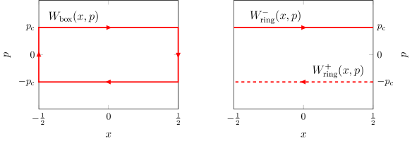
Let us briefly review the phase-space picture in the classical setting [18]. Heuristically, the joint (stationary) probability distribution of a classical particle of mass and energy which is confined in a box of unit length with elastically reflecting hard walls is given by
| (53a) | ||||
| (53b) | ||||
where , and corresponds to a rectangular orbit in the phase-space, see the left panel of Fig. 6. If the particle is confined in a ring, instead, we can consider two classical orbits, associated with the joint probability distributions
| (54) |
with and describing respectively a clockwise orbit and a counterclockwise one, see the right panel of Fig. 6.
Accordingly, the limit Wigner function introduced in Eq. (52), when it exists, can be interpreted from a classical perspective in two different ways. Since
| (55) |
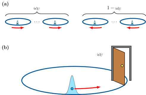
we can indeed consider as the probability distribution of a classical ensemble of particles in a ring, of which a fraction is moving clockwise whereas the remaining fraction is moving counterclockwise, see Fig. 7 (a).
Another interesting interpretation is suggested by the ergodic theorem [47]: can also represent the time-averaged probability distribution of a single classical particle in a ring with a junction, which acts as a door that can be opened or closed, allowing respectively the particle to pass through it or to be elastically reflected, thus inverting its motion, see Fig. 7 (b). In particular, in order to implement the limit distribution , each time the particle approaches the junction, the door has to be closed (and then subsequently reopened) with probability if the particle is moving clockwise, and with probability if it is moving counterclockwise. Notice however that, if the initial conditions are known, the probability distribution (55) can be also realized by a deterministic classical system.
4 Asymptotic analysis
In order to analyze the asymptotic behavior of the coefficients for large , we start by observing that Eq. (36) implies that
| (56) |
where
| (57a) | ||||
| (57b) | ||||
Notice that can vanish, as it happens for example when and (and thus ). Therefore there are two possibilities for , in the high-energy regime:
| (58a) | ||||
| (58b) | ||||
where , , and we used the fact that for .
We say that the sequence is balanced, when it admits the limit
| (59) |
and is unbalanced otherwise.
The balanced case can be easily characterized: Eq. (59) holds when
| (60a) | ||||
| (60b) | ||||
In turn, one can easily verify that these limits hold when one of the following sufficient conditions is satisfied.
-
1.
If and , that is if we consider the asymmetric Robin BCs
(61) then and for each . Remarkably, these are the most general local BCs. Notice that they can be either regular (if e.g , when they reduce to symmetric Robin BCs) and singular (if e.g. , which gives a mixed Dirichlet-Robin BC).
-
2.
If
(62) then and asymptotically as . As we will show in the next subsection, this spectral condition is always satisfied for regular BCs.
On the other hand, the study of the unbalanced case is more involved, and it requires the asymptotic estimate of the spectral quantities for large . Thus, we devote Sec. 4.1 to analyze in detail this spectral asymptotics. Then, in Sec. 4.2, after gathering the obtained results, we finally classify the possible classical limits of the Wigner functions .
4.1 Spectral asymptotics
By defining the sequence
| (63) |
the spectral condition in Eq. (62), that is relevant for the balanced case, is equivalent to
| (64) |
whereas the spectral quantities that are relevant for the unbalanced case can be rewritten as
| (65) |
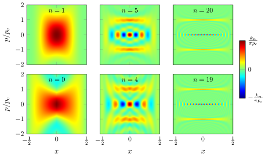
As it turns out, the behavior of can be quite erratic for small values of , but becomes more regular for large , see Fig. 8 for an example. The currently available spectral estimates associated with the Weyl law for quantum graphs [48, 49] are not enough to characterize the remainder term in Eq. (63), as they just imply that , for the system under study (which can be regarded as the “building block” of more complex quantum graphs). However, in the particular situation considered here, the asymptotic behavior of is known, see Sec. 1.5 of [50]. In this subsection we thus determine, on the lines of [50], the asymptotics of needed to analyze the limit of the coefficients .
To achieve this, let us rewrite the spectral function as
| (66) |
where and
| (67a) | ||||
| (67b) | ||||
| (67c) | ||||
It is convenient to separate the analysis into three cases:
-
•
BCs such that and hence for all (exact cases including Dirichlet BCs);
-
•
BCs such that and hence for all (singular BCs);
-
•
all the remaining BCs (regular BCs).
4.1.1 Exact cases.
We first consider the case of BCs such that for all . We show that this case occurs if and only if . In fact,
| (68) |
and
| (69) |
and hence . In this case we have that for all :
| (70) |
which clearly implies the spectral condition (62). Notice that the corresponding BCs are always regular.
4.1.2 Singular boundary conditions.
Let us now consider the singular BCs (22), i.e. . For this choice of parameters the spectral function simplifies to
| (71) |
and by considering the equation
| (72) |
which, since , can be rearranged as
| (73) |
we get
| (74) |
Notice that . In this case, one can show [50] that for large the sequence is asymptotically close to the sequence
| (75) |
In our notations, since , we can restrict to obtaining the asymptotic limits
| (76) |
and
| (77) |
Remarkably, for we recover the exact spectral sequence [25], that is:
| (78) |
For , in particular, the correction is constant:
| (79) |
Conversely, the limit (which gives Dirichlet BC) is ill-defined, and one should rely on the exact expression (70). We conclude that the asymptotic behavior of the sequence for singular BCs has a residual dependence on , and, for , also on the parity of .
4.1.3 Regular boundary conditions.
For what concerns the remaining (regular) BCs, we can now assume that , as the latter values have been discussed before. We rewrite the equation as
| (80) |
from which we get
| (81) |
Therefore for all :
| (82) |
Then, by using the fact that the wave numbers accumulate to , the above inequality implies the spectral condition in Eq. (62), that is
| (83) |
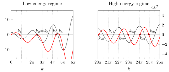
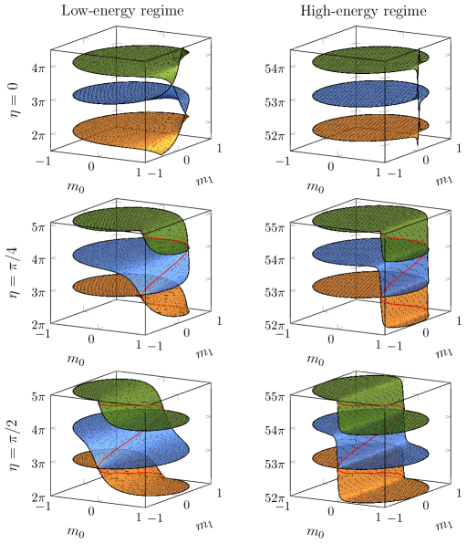
4.1.4 Numerical results.
To corroborate the asymptotic analysis, in Fig. 9 we plot the values of some wave numbers , which have been determined by numerically finding the zeroes of the spectral function, both in the low-energy regime (small ) and in the high-energy regime (large ), as function of the spectral parameters . The high-energy plots are consistent with the asymptotic formulas obtained so far. In Fig. 10 we also plot some exact values of in the high-energy regime, again as function of the spectral parameters . As expected, for (that is for regular BCs) we have that , while for we observe a residual dependence on , and in particular on .
4.2 Asymptotics of the Wigner function
To sum up, we obtained two sufficient conditions for having a balanced classical limit. Indeed, we found that if is a local BC, that is if for and , see Eq. (61), or if is a regular BC, so that the spectral condition in Eq. (62) is satisfied [see Eqs. (70) and (83)], then the coefficients have the well-defined high-energy limit
| (84) |
and the corresponding Wigner functions admit a limit in the form of Eq. (52) with balanced coefficients , that is:
| (85) |
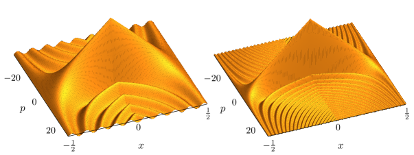
This balanced classical limit is represented, respectively for the case of Dirichlet and Neumann BCs, in the first and in the second row of Fig. 11.
For singular non-local BCs, instead, the situation is complicated by the fact that even in the high-energy regime the correction does generally still depend on the parity of , see Eqs. (76)–(77), thus not admitting a limit. However, since in the high-energy regime also the coefficients depend on only through its parity, see Eqs. (56)–(57) and (65), the following limits
| (86) |
are well-defined and finite. We stress that both and have a limit, but in general . Accordingly, although for singular non-local BCs the Wigner functions do not generally admit a classical limit, the even and odd subsequences have the well-defined limits in the form of Eq. (52),
| (87a) | ||||
| (87b) | ||||
with (generally) unbalanced coefficients and .
This phenomenon is shown in Fig. 12 for the family of “quasi-periodic” BCs , given by
| (88) |
In particular, these BCs reduce for to the pseudo-periodic BC , that is to and , and to the mixed Dirichlet-Neumann BC and for . Remarkably, for any , by using Eq. (79) we are able to get the simple exact expression
| (89) |
corresponding to the limit Wigner functions
| (90a) | ||||
| (90b) | ||||

5 Discussion and outlook
We showed that in the classical limit both local boundary conditions and regular boundary conditions are associated with a “balanced” ensemble, having a limit coefficient , so that the corresponding limit Wigner function coincides with the joint probability distribution of a classical particle in a box with elastically reflecting walls,
| (91) |
Notice that in the limit any information about the quantum boundary condition is lost. In this sense, the whole family of quantum systems with local and regular boundary conditions correspond to one and the same classical system.
For what concerns singular non-local boundary conditions, the situation is more elaborate, as the coefficients do not generally admit a limit, but oscillate between the limits of the the even and odd subsequences, that is between the values and defined in Eq. (86). The corresponding Wigner functions behave accordingly, with the even and odd subsequences having the limit Wigner functions and given by Eqs. (87). These latter distributions have exactly the form (55), in general with an unbalanced coefficient carrying a residual information—a classical echo—of the quantum boundary condition . As we discussed in Sec. 3.3, in this case, for a given parity, the limit Wigner function can be interpreted as the probability distribution of an ensemble of classical particles in a ring, with a fraction moving clockwise and a fraction moving counterclockwise.
We conclude with some outlooks. In this Article we have analyzed the classical limit for the eigenfunctions of the non-relativistic kinetic-energy operator in a one-dimensional box with general self-adjoint boundary conditions. The corresponding classical distribution probabilities are stationary, i.e. time-independent. Performing a similar analysis by considering suitable wave packets, instead of the eigenfunctions, we expect to obtain a different classical distribution [51, 18] mimicking a classical dynamical orbit. Future research will be devoted to this subject. Besides, more generally, it is still an open question if in the classical limit different self-adjoint extensions of a given operator all collapse (in a suitable sense) to the same classical object. One could investigate this problem by looking at the asymptotic behavior of the symbols associated with the different self-adjoint extensions of the operator [44, 45]. Other interesting generalizations of the present work may involve the analysis of a particle with spin and of a relativistic particle in a box (with general boundary conditions) [52, 53, 54], as well as the case of multiple particles [55].
Acknowledgments
This work was partially supported by Istituto Nazionale di Fisica Nucleare (INFN) through the project “QUANTUM”, by PNRR MUR Project PE0000023-NQSTI, by Regione Puglia and QuantERA ERA-NET Cofund in Quantum Technologies (Grant No. 731473), project PACE-IN, by the Italian National Group of Mathematical Physics (GNFM-INdAM), and by the Italian funding within the “Budget MUR - Dipartimenti di Eccellenza 2023–2027” - Quantum Sensing and Modelling for One-Health (QuaSiModO).
References
References
- [1] E. Wigner, On the quantum correction for thermodynamic equilibrium, Phys. Rev. 40, 749–759 (1932).
- [2] M. Hillery, R.F. O’Connell, M.O. Scully and E.P. Wigner, Distribution functions in physics: Fundamentals, Phys. Rep. 106, 121–167 (1984).
- [3] H.-W. Lee, Theory and application of the quantum phase-space distribution functions, Phys. Rep. 259, 3 (1995).
- [4] G.G. Cabrera and M. Kiwi, Large quantum-number states and the correspondence principle, Phys. Rev. A 36, 6 (1987).
- [5] G.Q. Hassoun and D.H. Kobe, Synthesis of the Planck and Bohr formulations of the correspondence principle, Am. J. Phys. 57, 658–662 (1989).
- [6] V.I. Man’ko, G. Marmo, A. Simoni, A. Stern and F. Ventriglia, Tomograms in the quantum-classical transition, Phys. Lett. A 343, 4 251–266 (2005).
- [7] B. Koczor, R. Zeier and S.J. Glaser, Continuous phase-space representations for finite-dimensional quantum states and their tomography, Phys. Rev. A 101, 022318 (2020).
- [8] M. Przanowski, P. Brzykcy and J. Tosiek, From the Weyl quantization of a particle on the circle to number-phase Wigner functions, Ann. Phys. 351, 919–934 (2014).
- [9] K. Kowalski and K. Ławniczak, Wigner functions and coherent states for the quantum mechanics on a circle, J. Phys. A: Math. Theor. 54, 275302 (2021).
- [10] S. Zhang and A. Vourdas, Phase space methods for particles on a circle, J. Math. Phys. 44, 5084 (2003).
- [11] I. Rigas, L.L. Sánchez-Soto, A.B. Klimov, J. Řeháček, Z. Hradil, Orbital angular momentum in phase space, Ann. Phys. 326, 2 (2011).
- [12] M. Ligabò, Torus as phase space: Weyl quantization, dequantization, and Wigner formalism, J. Math. Phys. 57, 082110 (2016).
- [13] N.C. Dias J.N. Prata Wigner functions with boundaries, J. Math. Phys. 43, 4602 (2002).
- [14] S. Kryukov and M.A. Walton, On infinite walls in deformation quantization, Ann. Phys. 317, 474–491 (2005).
- [15] N.C. Dias and J.N. Prata, Deformation quantization of confined systems, Int. J. Quantum Inf. 05, 257–263 (2007).
- [16] N.C. Dias, A. Posilicano and J.N. Prata, Self-adjoint, globally defined Hamiltonian operators for systems with boundaries, Comm. Pure Appl. Math. 10, 6 (2011).
- [17] M. Casas, H. Krivine and J. Martorell, On the Wigner transforms of some simple systems and their semiclassical interpretation, Eur. J. Phys. 12, 105 (1991).
- [18] M. Belloni, M.A. Doncheski and R.W. Robinett, Wigner quasi-probability distribution for the infinite square well: Energy eigenstates and time-dependent wave packets, Am. J. Phys. 72, 1183–92 (2004).
- [19] M.A. Walton, Wigner functions, contact interactions, and matching, Ann. Phys. 322, 9 (2007).
- [20] M.H. Al-Hashimi and U.-J. Wiese, Canonical quantization on the half-line and in an interval based upon an alternative concept for the momentum in a space with boundaries, Phys. Rev. Research 3, 033079 (2021).
- [21] R.W. Robinett, Quantum and classical probability distributions for position and momentum, Am. J. Phys. 63, 9 (1995).
- [22] R.W. Robinett, Visualizing classical and quantum probability densities for momentum using variations on familiar one-dimensional potentials, Eur. J. Phys. 23, 165 (2002).
- [23] J. Bernal, A. Martín-Ruiz and J. García-Melgarejo, A Simple Mathematical Formulation of the Correspondence Principle, J. Mod. Phys. 4, 1 (2013).
- [24] G. Teschl, Mathematical methods in quantum mechanics, Graduate Studies in Mathematics, American Mathematical Society (2014).
- [25] G. Bonneau, J. Faraut and G. Valent, Self-adjoint extensions of operators and the teaching of quantum mechanics, Am. J. Phys. 69, 3 (2001).
- [26] M. Asorey, A. Ibort and G. Marmo, Global theory of quantum boundary conditions and topology change, Int. J. Mod. Phys. A 20, 1001–1025 (2005).
- [27] M. Asorey, A. Ibort and G. Marmo, The topology and geometry of self-adjoint and elliptic boundary conditions for Dirac and Laplace operators, Int. J. Geom. Methods Mod. Phys. 12, 06 (2015).
- [28] A. Ibort, F. Lledó and J.M. Pérez-Pardo, Self-adjoint extensions of the Laplace-Beltrami operator and unitaries at the boundary, J. Funct. Anal. 268, 3 634–670 (2015).
- [29] P. Facchi, G. Garnero and M. Ligabò, Self-adjoint extensions and unitary operators on the boundary, Lett. Math. Phys. 108, 195–212 (2018).
- [30] W.B. Case, Wigner functions and Weyl transforms for pedestrians, Am. J. Phys. 76, 937–946 (2008).
- [31] P. Facchi, G. Garnero and M. Ligabò, Quantum cavities with alternating boundary conditions, J. Phys. A: Math. Theor. 51, 105301 (2018).
- [32] B. Belchev and M.A. Walton, On Robin boundary conditions and the Morse potential in quantum mechanics, J. Phys. A: Math. Theor., 43, 8 (2010).
- [33] A. Balachandran, G. Bimonte, G. Marmo, and A. Simoni, Topology change and quantum physics, Nucl. Phys. B 446, 299–314 (1995).
- [34] A.D. Shapere, F. Wilczek, and Z. Xiong, Models of Topology Change, arXiv: 1210.3545 [hep-th] (2012).
- [35] M. Asorey, P. Facchi, G. Marmo, and S. Pascazio, A dynamical composition law for boundary conditions, J. Phys. A: Math. Theor. 46, 102001 (2013).
- [36] A. Ibort, F. Lledó, and J.M. Pérez-Pardo, Self-adjoint extensions of the Laplace-Beltrami operator and unitaries at the boundary, J. Funct. Anal. 268, 634–670 (2015).
- [37] P. Facchi, G. Garnero, G. Marmo, J. Samuel, and S. Sinha, Boundaries without boundaries, Ann. Phys. 394, 139–154 (2018).
- [38] S. Di Martino, F. Anzà, P. Facchi, A. Kossakowski, G. Marmo, A. Messina, B. Militello and S. Pascazio, A quantum particle in a box with moving walls, J. Phys. A: Math. Theor. 46, 365301 (2013).
- [39] S. Di Martino and P. Facchi, Quantum systems with time-dependent boundaries, Int. J. Geom. Methods Mod. Phys. 12, 1560003 (2015).
- [40] G. Angelone, P. Facchi and G. Marmo, Hearing the shape of a quantum boundary conditions, Mod. Phys. Lett. A 37, 2250114 (2022).
- [41] A. Zettl, Sturm-Liouville Theory, Mathematical surveys and monographs, American Mathematical Society (2005).
- [42] J. Mostowski and J. Pietraszewicz, Wigner Function for Harmonic Oscillator and The Classical Limit, arXiv:2104.06638 [quant-ph] (2021).
- [43] V. Moretti and C.J.F. van den Ven, The classical limit of Schrödinger operators in the framework of Berezin quantization and spontaneous symmetry braking as an emergent phenomenon, Int. J. Geom. Methods Mod. Phys. 19, 01 (2022).
- [44] F.D. Cunden, P. Facchi and M. Ligabò, The semiclassical limit of a quantum Zeno dynamics, Lett. Math. Phys. 113, 114 (2023).
- [45] F.D. Cunden, M. Ligabò and M. C. Susca, Truncated quantum observables and their semiclassical limit, in preparation (2024).
- [46] M.J. Lighthill, An Introduction to Fourier Analysis and Generalised Functions, Cambridge University Press (1958).
- [47] C.C. Moore, Ergodic theorem, ergodic theory, and statistical mechanics, Proceedings of the National Academy of Sciences 112, 7 1907–1911 (2015).
- [48] J. Bolte, S. Endres, The Trace Formula for Quantum Graphs with General Self Adjoint Boundary Conditions, Ann. Henri Poincaré 10, 189–223, (2009).
- [49] A. Odžak, L. Šćeta, On the Weyl Law for Quantum Graphs, Bull. Malays. Math. Sci. Soc. 42, 119–131 (2019).
- [50] V.A. Marchenko, Sturm-Liouville Operators and Applications, Birkhäuser Basel (1986).
- [51] C. Leubner, M. Alber and N. Schupfer, Critique and correction of the textbook comparison between classical and quantum harmonic oscillator probability densities, Am. J. Phys. 56, 1123–1129 (1988).
- [52] G.R. Shin, I. Bialynicki-Birula and J. Rafelski, Wigner function of relativistic spin-1/2 particles, Phys. Rev. A 46, 645 (1992).
- [53] K. Kowalski and J. Rembieliński, The Wigner function in the relativistic quantum mechanics, Ann. Phys. 375, 1–15 (2016).
- [54] G. Angelone, Hearing the boundary conditions of the one-dimensional Dirac operator, arXiv:2311.17561 [quant-ph] (2023).
- [55] B. De Bruyne, D.S. Dean, P. Le Doussal, S.N. Majumdar and G. Schehr, Wigner function for noninteracting fermions in hard-wall potentials, Phys. Rev A 104, 013314 (2021).