Separation capacity of linear reservoirs with random connectivity matrix

Abstract.

We argue that the success of reservoir computing lies within the separation capacity of the reservoirs and show that the expected separation capacity of random linear reservoirs is fully characterised by the spectral decomposition of an associated generalised matrix of moments. Of particular interest are reservoirs with Gaussian matrices that are either symmetric or whose entries are all independent. In the symmetric case, we prove that the separation capacity always deteriorates with time; while for short inputs, separation with large reservoirs is best achieved when the entries of the matrix are scaled with a factor $\rho_{T}/\sqrt{N}$, where $N$ is the dimension of the reservoir and $\rho_{T}$ depends on the maximum length of the input time series. In the i.i.d. case, we establish that optimal separation with large reservoirs is consistently achieved when the entries of the reservoir matrix are scaled with the exact factor $1/\sqrt{N}$. We further give upper bounds on the quality of separation in function of the length of the time series. We complement this analysis with an investigation of the likelihood of this separation and the impact of the chosen architecture on separation consistency.

1. Introduction

1.1. The reservoir computing paradigm

Recurrent neural networks (RNNs) were one of the earliest machine learning architectures specifically tailored for processing sequential data streams. They are able to track long term temporal dependencies and to handle variable-length data, such as financial time series or text. In contrast to feed-forward neural networks (FFNN), RNNs are composed of relatively few neurons connected in a strongly recurrent manner. The building block of RNNs is mapping input time series (of any length) to a hidden state of fixed length (using the same set of parameters and thus accounting for temporal dependencies), which is then fed to another parametric map (e.g., a regression map or a classifier). More formally, given a $d$-dimensional time series $\mathbf{x}=(x_{t})_{0\leq t\leq T}\in(\mathbb{R}^{d})^{(T+1)}$, the output $\mathbf{y}=(y_{t})_{0\leq t\leq T}\in(\mathbb{R}^{n})^{(T+1)}$ of a basic RNN is computed sequentially as follows

(1) $$\left\{\begin{array}[]{ll}z_{0}=\sigma(ux_{0})\in\mathbb{R}^{N},\\ z_{t}=\sigma(Wz_{t-1}+ux_{t})\in\mathbb{R}^{N},&\text{for all }1\leq t\leq T,\\ y_{t}=h(z_{t})\in\mathbb{R}^{n},\\ \end{array}\right.$$

where $u\in\mathbb{R}^{N\times d}$ is a pre-processing matrix, $W\in\mathbb{R}^{N\times N}$ -called the connectivity matrix- models the connection strength between neurons, $\sigma:\mathbb{R}\to\mathbb{R}$ is an activation function applied element-wise and $h$ is a parametric map (e.g. a hyperplane classifier or a standard FFNN.) In principle, and very much like in a classical FFNN, all the parameters $u$, $W$ and $h$ can be optimised, using a gradient descent algorithm, by minimising a suitable empirical risk function applied to a training dataset. However, it is shown both theoretically and practically that such algorithms may either fail to converge, or do converge toward a saddle point ([Doy92, BFS93, LHEL21]), more frequently than in classical FFNNs. In particular, and due to the recurrent nature of the architecture, the final hidden state $z_{T}$ involves $T-t$ applications of the connectivity matrix $W$ on the past input value $x_{t}$, for all $t\in[\![0,T]\!]$. Thus, when handling very long time series, optimising $W$ can easily lead to numerical instability problems and a terminal state of the network that fails to appropriately take into account the contribution of the early terms of the data streams.

Two of the most successful innovations to improving the performance of RNNs were the introduction of gating (e.g. Long Short-Term Memory networks (LSTMs, [HS97]) and Gated Recurrent Units (GRUs, [JGP⁺19])) and attention (e.g. Transformers, [VSP⁺17].) However, the well documented empirical success of such techniques comes at a high computational cost and, most importantly, a lack of theoretical analysis and guarantees and adequate interpretation.

An alternative approach, reservoir computing, proposed in [JH04] and [MJS07], offers a simpler yet effective solution. In reservoir computing, the connectivity matrix $W$ is randomly chosen rather than learned. In this context, the map $\mathbf{x}\mapsto\mathbf{z}=(z_{t})_{0\leq t\leq T}$ is called a reservoir, $W$ the reservoir matrix, and $N$ the reservoir dimension (although these appellations are not strictly reserved to this paradigm). Typically, $N$ is chosen to be very large and $W$ to have either its largest singular value or its spectral radius close to but strictly smaller than 1. This type of networks is much easier to train: only $h$, and sometimes $u$, are learned; in some implementations, e.g. [DCR⁺18], even $u$ is randomly generated. Additionally, reservoir computers have shown excellent performances in practice ([JH04, SH06]) and are even implemented in hardware (e.g. [ASVdS⁺11, LKDB18, VMVV⁺14]) due to their muti-tasking abilities (since only few parameters need to be retrained in function of the task at hand.)

1.2. Mathematical foundations of reservoir computing

Despite its empirical success, a comprehensive and rigorous mathematical explanation for the effectiveness of reservoir computing remains elusive. Nonetheless, recent research efforts have made strides in partially analysing these systems from various perspectives and under different mathematical assumptions, though these may not always reflect the reality of the data streams or the systems to learn. Let us mention four sets of recent results that are relevant to the present work and that have shed some light onto our mathematical understanding of the functioning of reservoir computing and, more generally, recurrent neural networks.

Kernel Machine Analogy. Using an analogy with classical kernel techniques in machine learning, the authors in [Tin20, VALT22] view each reservoir state $z_{t}$ as the realisation of a feature map on the previous input states $(x_{s})_{0\leq s\leq t}$. Thus, reservoirs can be seen as kernel machines with Gram matrices characterised by the powers $W^{n}$ of the connectivity matrix $W$. Applying the Cayley-Hamilton theorem, i.e. that for all $n\in\mathbb{N}$, there exists a collection of real numbers $(a_{i,n})_{0\leq i\leq N-1}$ (that can be computed inductively) such that

$$W^{n}=\sum_{i=0}^{N-1}a_{i,n}W^{i},$$

one can simplify the understanding of the behaviour of such kernel machines by understanding the re-expansion of the reservoir state $z_{t}$ in terms of the first $N$ powers of $W$ only. In certain cases, such as when $W$ is (up to a multiplication by a constant hyperparameter) the cyclic matrix

$$W=\left(\begin{array}[]{cccccc}0&0&0&\cdots&0&1\\ 1&0&0&\cdots&0&0\\ 0&1&0&\cdots&0&0\\ \vdots&\vdots&\vdots&\cdots&\vdots&\vdots\\ 0&0&0&\cdots&1&0\\ \end{array}\right),$$

the terms $(a_{i,n})_{0\leq i\leq N-1}$, for all $n\in\mathbb{N}$, can be computed explicitly. Consequently, the dependence of the reservoir state on recent and distant past input entries becomes well-understood.

Universal Approximation Properties. In [GO18a], it is shown that, under appropriate assumptions, recurrent neural networks possess universal approximation properties. More specifically, any continuous map $\mathbf{x}\mapsto y\in\mathbb{R}$ can be approximated arbitrarily well in the uniform continuity topology over a compact set of input states by suitably adjusting the architecture parameters. Here, the sequences of states are modelled as infinite sequences and the well-posedness of the system (1) is ensured by assuming the reservoir mapping $\mathbf{x}\mapsto\mathbf{z}$ to be contractive. Similar results under different mathematical modelling assumptions can be found for example in [BC85, GO20, GGO23]. As in many universal approximation theorems, most of these results rely on a judicious application of the Stone-Weierstrass theorem.

Stochastic algorithms. The application of stochastic algorithms with randomly generated parameters in contrast to deterministic algorithms with learned parameters is certainly not a new idea in data science and machine learning. The most known example of such applications is perhaps the Johnson-Lindenstrauss lemma (see for instance [JL84, DG03, Ver18]) where one is interested in finding a linear mapping $A$ such that $N$ given points $x_{1},x_{2},\ldots,x_{N}$ in a high-dimensional space $\mathbb{R}^{n}$ are projected onto a lower dimensional space $\mathbb{R}^{m}$ while almost preserving their pairwise distances, i.e.

(2) $$\forall i,j\in[\![1,N]\!]\colon\quad(1-\varepsilon)\|x_{i}-x_{j}\|_{2}\leq\|Ax_{i}-Ax_{j}\|_{2}\leq(1+\varepsilon)\|x_{i}-x_{j}\|_{2},$$

for a given error $\varepsilon\in(0,1)$. Remarkably, this problem can be solved easily (and “cheaply”) with high probability without “learning” $A$ in function of the data $x_{1},x_{2},\ldots,x_{N}$. For example, one may choose $A$ to be the orthogonal projection onto an $m$-dimensional subspace that is chosen randomly (according to the uniform Haar probability measure on the Grasmannian $G_{n,m}$). Alternatively, one may choose $A\in\mathbb{R}^{m\times n}$ with i.i.d. centred Gaussian entries with variance $1/m$. Naturally, $m$ depends on $\varepsilon$, $N$ and the probabilistic margin error (with which we want (2) to hold.) However, $m$ depends neither on the data $x_{1},x_{2},\ldots,x_{N}$ nor on the dimension $n$. Another illustration of the effectiveness of random algorithms can be given in the context of FFNNs. For instance, [DGJS22] shows that an FFNN with 2 hidden layers, the ReLU activation function and randomly generated parameters can, with high probability, linearly separate non-linear sets. This study continues on a line of research into the potential of machine learning techniques with random features, see for instance [GS20, GGT23, CGG⁺22].

Choice of the connectivity matrix. The argument of choosing the connectivity matrix $W$ to have either its largest singular value or its spectral radius strictly smaller than 1 is usually motivated by a numerical stability argument (or by a theoretical contractivity condition). However, when $W$ is randomly sampled according to a probability distribution, this justification may lose its relevance. Moreover, the decision of the choice between the operator norm and the spectral radius requires careful justification. In practice, the entries of the $N\times N$ matrix $W$ (with $N$ being very large) are chosen to be centred Gaussian distributions with variance $\frac{1}{N}$ (or, more precisely, $\frac{\rho^{2}}{N}$, with $\rho$ close to but strictly smaller than 1.) The entries of $W$ are usually chosen to all be independent or such that $W$ is symmetric with independent entries in its upper-triangular part. Within the physics community, this choice of distribution and variance is usually traced back to an argument in [SCS88], which does not go into details of the reasons of this choice. The book [HD20] is an attempt to justify such choices from the lens of statistical field theory. Loosely speaking, a variance of order $\frac{1}{N}$ results in a disorder-averaged generating functional that is independent of $N$. The same reference justifies the use of large $N$ for interpretability reasons: when $N$ is large enough for the “central limit” regime to kick in, employing results from mean field theory becomes justifiable, thus allowing for a better understanding of the network’s behaviour through this lens.

1.3. Current theoretical limitations

Despite these recent advances, the scope of success of reservoir computing is still far from being fully explained by the existing theories. For example, many works rely on results from the theory of dynamical systems by representing the time series $\mathbf{x},\mathbf{z}$ and $\mathbf{y}$ as (semi-)infinite series and assuming either the function to learn or the RNN itself to be contractive in $\mathbf{x}$ (thus ensuring that the system (1) is well-posed for infinite sequences.) This condition, known as the echo state property, ensures numerical stability and independence of outputs from distant past inputs. However, this framework does not apply to or reflect the reality of systems that handle relatively short (but possibly varying-length) sequences (like in speech recognition), or systems whose output depend heavily on the initial input states. For instance, when processing the sentence “What time is it?”, the key information is contained at the start of the sentence “What time”. Another simple toy example is a system that is fed the changes in stock prices through time instead of the price itself. In this last example, the system does not satisfy the echo state property and the whole history of the time series may be necessary for approximating functions of the stock price (such as the price of a European call option on that stock). Moreover, the well-posedness of the system (1) -which depends fully on the choice of norms on time series spaces- is not questioned in practice, where time series are never infinite. Another relatively popular working condition that shares similar drawbacks is the assumption that the functional to learn can be well approximated using only the near past. This allows one to leverage classical results for FFNNs as, under this assumption, the time series can be well approximated by a fixed length vector containing only the near past inputs.

Another prevalent gap in the existing literature is that the sampling distribution of the connectivity matrix is never fully taken into account. Thus the dependence of the properties of the random reservoir on the choice of the generating distribution and the dimension $N$ is poorly understood. For example, what is the reason behind the empirical success of choosing the connectivity matrix $W$ to have Gaussian entries (or entries uniformly distributed over an interval) with variances scaling in $1/N^{2}$? Why does the choice of large values for $N$ tend to give better results? What difference in performance can we expect between a choice of $W$ with independent entries or a symmetric $W$ with independent upper-diagonal entries? In several previous attempts to answer some of these questions, deterministic properties are assumed to hold for the matrix $W$ based on asymptotic expected properties (such as the expected operator norm); which, as we will see across this paper, can be a misleading intuition.

1.4. Contributions and organisation of the paper

In this study, we aim to explain the success of reservoir computing by its separation capacity: given two time series with different outputs, then, naturally, their associated reservoir states must be distinct as a necessary condition for the RNN to be able to correctly compute or approximate their outputs. In order to build intuition and provide accurate results, we will make an important simplification by taking the activation function $\sigma$ to be the identity. However, this does not hinder the performance of the RNN as such a network can still have universal approximation properties by choosing $h$ to be a polynomial for example, as shown in [GO18b] (Corollary 11). In a practical context, such a linear reservoir was implemented and studied in [LKDB18]. We will reason that, in the same way that a random Gaussian matrix constitutes a cheap almost isometric projection map in the Johnson-Lindenstrauss’ lemma, random connectivity matrices sampled according to a suitable distribution are able to associate, on average, different reservoir states to different time series (or different reservoir states for a single time series through time). We investigate and quantify the impact of the choice of the sampling distribution and the dimension of the reservoir on the separation capacity of the random linear reservoir, along with the potential influence of time towards the degradation of this capacity. More particularly, we will proceed in the paper in the following manner. Section 2 introduces the mathematical model, general assumptions, and notations of the paper, along with some preliminary remarks. In Section 3, we examine the expected squared distance between reservoir states associated with two time series. Starting with the 1-dimensional case, we first prove that this expected separation capacity is fully characterised by the matrix of moments of the connectivity distribution (Theorem 1). As a corollary, we show that a choice of a connectivity distribution with infinite support, for instance Gaussian, guarantees separability (Proposition 2). However, in the Gaussian case, we show that this separation capacity is bound to deteriorate when dealing with long time series, as either some components of the input time series get increasingly ignored by the reservoir or contribute significantly less to the distances between outputs (Theorem 5). The choice of the variance of the connectivity (small or large), thought of as a hyperparameter, can only lightly alleviate one of the two deteriorations. In Subsection 3.2, we generalise most of the previous results to higher dimensional reservoirs; for instance, that the expected separation capacity is characterised by a generalised matrix of moments (Theorem 6). The purpose here is to study the impact of the practical implementation variables and choices -such as the reservoir dimension, generating distribution of the connectivity matrix and any symmetry assumptions thereon- on the separation capacity of the reservoir. While the results and the techniques generalise to a larger class of connectivity matrices, we will focus on the most widely used case of Gaussian connectivity matrices, more particularly the case where the random connectivity matrix $W\in\mathbb{R}^{N\times N}$ either has independent entries or is symmetric with independent entries on and above the diagonal. In practice, the standard deviation of the entries of $W$ is usually chosen to be $\frac{\rho}{\sqrt{N}}$, with $N$ very large and $\rho$ close to but smaller than $1$. To understand the implications of this choice, we will consider a larger class of scalings of the type $\frac{\rho}{N^{\alpha}}$, where $\alpha\in\mathbb{R}$. In the symmetric case, we show that the expected separation capacity of the reservoir is bound to deteriorate for long time series, irrespective of the chosen scaling (Theorem 18). For relatively short time series, a balanced separation (for all time series) is only achieved for scalings close to the classical scaling $1/\sqrt{N}$ when $N$ is chosen to be large (Theorem 14). In the i.i.d. case, we show that separation is universally best achieved for exactly the classical scaling $1/\sqrt{N}$ when $N$ is very large (Theorem 21). We also obtain upper bounds for the quality of separation of very long time series (Theorem 24) that suggest that scalings with $\sigma$ very far from $1/\sqrt{N}$ result in a rapid deterioration of separability with time. On the other hand, matrices with a scaling $\sigma\approx 1/\sqrt{N}$ exhibit the best separability properties, especially if $N\gg T$. Section 4 completes the results about the expected distance distortion by quantifying the probability of separation. Starting again with the 1-dimensional case, we prove that one may always multiply any random connectivity with a large hyperparameter to ensure separation of the outputs with arbitrarily large probability. In the general high-dimensional case, we highlight the dependence of the distribution of the expected (square) distance around its mean on both the data and the architecture. Using a numerical example, we note that, when using connectivity matrices with i.i.d. entries, the (square) distances between reservoir states seem to be better concentrated around their means compared to the case of symmetric matrices, thus resulting in more consistent results.

2. Notations and general remarks

$\mathbb{N}$ (respectively $\mathbb{N}^{*}$) denotes the set of positive integers (resp. strictly positive integers.) Given $d\in\mathbb{N}^{*}$, consider $d$-dimensional input time series

$$\mathbf{x}=(x_{t})_{0\leq t\leq T}\in(\mathbb{R}^{d})^{(T+1)}=(x_{0},x_{1},\ldots,x_{T}),$$

where, for $0\leq t\leq T$, $x_{t}$ is the information received at time $t$. At each time $t$, the signal $x_{t}$ is transformed into an $N$-dimensional vector by a pre-processing matrix $u\in\mathbb{R}^{N\times d}$, with $N\in\mathbb{N}^{*}$. The linear reservoir with dimension $N$ and random connectivity matrix $W\in\mathbb{R}^{N\times N}$ associates a reservoir state (or hidden state) $f_{t}(\mathbf{x},W)\in\mathbb{R}^{N}$ to such a time series computed recursively as follows

$$\left\{\begin{array}[]{ll}f_{0}(\mathbf{x},W)=ux_{0}\in\mathbb{R}^{N},\\ f_{t}(\mathbf{x},W)=Wf_{t-1}(\mathbf{x},W)+ux_{t}\in\mathbb{R}^{N},&\text{for all }1\leq t\leq T.\\ \end{array}\right.$$

Note that, at time $t$, the reservoir state $f_{t}(\mathbf{x},W)$ is given by the simple formula

$$f_{t}(\mathbf{x},W)=ux_{t}+Wux_{t-1}+\cdots+W^{t}ux_{0}=\sum_{s=0}^{t}W^{s}ux_{t-s}.$$

In particular, $f_{t}(\cdot,W)$ is linear. Hence, comparing the following distance of the reservoir states

$$\|f_{t}(\mathbf{x},W)-f_{t}(\mathbf{y},W)\|_{2}$$

to the Euclidean distance $\|\mathbf{x}-\mathbf{y}\|_{2}$, where $\mathbf{x}$ and $\mathbf{y}$ are two given input time series, is equivalent to understanding the link between $\|f_{t}(\mathbf{a},W)\|_{2}$ and $\|\mathbf{a}\|_{2}$ for any given input time series $\mathbf{a}$: one needs only to consider $\mathbf{a}:=\mathbf{x}-\mathbf{y}$.
Next, we note that the reservoir state $f_{t}(\mathbf{x},W)$ associated with a time series $\mathbf{x}$ at time $t$ can be written as the final reservoir state at time $T$ associated with the delayed time series $\tau_{t}(\mathbf{x})$ where the first $T-t$ input values are equal to $0$, i.e.

$$\tau_{t}(\mathbf{x}):=(0,\ldots,0,x_{0},x_{1},\ldots,x_{t}).$$

More precisely

$$\begin{array}[]{rcl}f_{t}(\mathbf{x},W)&=&ux_{t}+Wux_{t-1}+\cdots+W^{t}ux_{0}\\ &=&ux_{t}+Wux_{t-1}+\cdots+W^{t}ux_{0}+W^{t+1}u\cdot 0+\cdots+W^{T}u\cdot 0\\ &=&f_{T}((0,\ldots,0,x_{0},x_{1},\ldots,x_{t}),W).\\ \end{array}$$

Consequently, understanding the change in time in reservoir states $f_{t+1}(\mathbf{x},W)-f_{t}(\mathbf{x},W)$ for a single time series $\mathbf{x}$ is equivalent to understanding the difference in terminal reservoir states

$$f_{T}(\tau_{t+1}(\mathbf{x}),W)-f_{T}(\tau_{t}(\mathbf{x}),W)$$

associated to the delayed time series $\tau_{t+1}(\mathbf{x})$ and $\tau_{t}(\mathbf{x})$.

In light of the above arguments, we will then restrict ourselves in this paper to studying the separation properties of the final reservoir state map $f:=f_{T}$.
Finally, as we are interested in the separation capacity of a reservoir when looking at time series as a vector with entries given by their values through time, i.e. the ratio

$$\frac{\|f(\mathbf{a},W)\|_{2}}{\|\mathbf{a}\|_{2}},\text{ for }\mathbf{a}\neq\mathbf{0},$$

and as we are not considering the $d$-dimensional spacial distribution of the signals then, without loss of generality, we will limit ourselves to $1$-dimensional input time series (i.e. $d=1$ and $\mathbf{a}\in\mathbb{R}^{T+1}$) and we will assume that $u=(1,\ldots,1)^{\top}$. This is line with the working assumptions in [VALT22, Tin20] for instance.

Let us end this section with further notation that is key in this paper. For two integers $p\leq q$, $[\![p,q]\!]$ denotes the set $\{p,p+1,\ldots,q\}$. Given $N\in\mathbb{N}^{*}$, we denote $[N]=[\![1,N]\!]$. Given a vector $x=(x_{1},\ldots,x_{d})\in\mathbb{R}^{d}$, $\|x\|_{2}$ denotes its Euclidean norm, i.e.

$$\|x\|_{2}^{2}=\sum_{i=1}^{d}x_{i}^{2}.$$

$A^{\top}$ denotes the transpose of a given matrix $A$. Given $m,n\in\mathbb{N}^{*}$ and a matrix $A\in\mathbb{R}^{m\times n}$, $\left\|A\right\|_{\mathrm{op}}$ denotes the operator norm of $A$

$$\left\|A\right\|_{\mathrm{op}}=\max_{x\in\mathbb{R}^{n}\setminus\{0\}}\frac{\|Ax\|_{2}}{\|x\|_{2}},$$

while $\|A\|_{2,\infty}$ denotes the following induced norm

$$\|A\|_{2,\infty}=\max_{1\leq i\leq m}\|A_{i\cdot}\|_{2}=\max_{1\leq i\leq m}\left(\sum_{1\leq j\leq n}A_{ij}^{2}\right)^{1/2}.$$

Given $n\in\mathbb{N}^{*}$ and a matrix $A\in\mathbb{R}^{n\times n}$, $\mathrm{tr}(A)$ denotes the trace of $A$. When no confusion is possible, $|X|$ denotes the number of elements in a given finite set $X$. Given two strictly positive sequences $(x_{t})_{t\in\mathbb{N}}$ and $(y_{t})_{t\in\mathbb{N}}$, we write $x_{t}\underset{T\to+\infty}{\simeq}y_{t}$ if $\left(\frac{x_{t}}{y_{t}}\right)_{t\in\mathbb{N}}$ converges to 1 at infinity. Finally, $X\sim\mathcal{N}(m,\sigma^{2})$ means that $X$ is a Gaussian random variable with mean $m$ and variance $\sigma^{2}$.

3. Expected distance distortion

In this section, we will study the properties of the expectation of the ratio $\frac{\|f(\mathbf{a},W)\|_{2}}{\|\mathbf{a}\|_{2}}$ (or more accurately, the expectation of its square) for $\mathbf{a}\in\mathbb{R}^{T+1}$ and $W$ is random. We will start by looking at the temporal behaviour of such ratio as $T$ tends to infinity in the one-dimensional case $N=1$ where more results can be stated or accurately obtained. In the higher dimensional case, we will look at both limit cases $T\to\infty$ and $N\to\infty$.

3.1. The 1-dimensional case

For a one-dimensional signal $\mathbf{x}:=(x_{t})_{0\leq t\leq T}$, the output of the reservoir with random connectivity $w$ (in this case a one-dimensional random variable) is given by

$$f(\mathbf{x},w)=\sum_{t=0}^{T}x_{T-t}w^{t}.$$

Let us first show a fundamental and straightforward theorem characterising the separation capacity of this random reservoir, which will form the basis of much of the study in this subsection.

Theorem 1.

Consider a one-dimensional linear reservoir with random connectivity $w$, i.e. the output of the reservoir for the signal $\mathbf{x}:=(x_{t})_{0\leq t\leq T}$ is given by

$$f(\mathbf{x},w)=\sum_{t=0}^{T}x_{T-t}w^{t}.$$

Then the expected separation capacity of the reservoir is characterised by the eigenvalues of the symmetric positive semi-definite matrix

$$B_{T}:=(\mathbb{E}w^{i+j})_{0\leq i,j\leq T}.$$

More specifically, if $\lambda_{\mathrm{min}}(B_{T})$ and $\lambda_{\mathrm{max}}(B_{T})$ denote respectively the smallest and largest eigenvalue of $B_{T}$, and given two time series $\mathbf{x}$ and $\mathbf{y}$, one has

(3) $$\lambda_{\mathrm{min}}(B_{T})\|\mathbf{x}-\mathbf{y}\|^{2}_{2}\leq\mathbb{E}(f(\mathbf{x},w)-f(\mathbf{y},w))^{2}\leq\lambda_{\mathrm{max}}(B_{T})\|\mathbf{x}-\mathbf{y}\|^{2}_{2}.$$

Proof.

Given two time series $\mathbf{x}$ and $\mathbf{y}$, and defining $\mathbf{a}:=\mathbf{x}-\mathbf{y}$, we get

$$f(\mathbf{x},w)-f(\mathbf{y},w)=f(\mathbf{a},w)=B_{T}(w)^{\top}a,$$

where

$$B_{T}(w):=\left(1,w,\ldots,w^{T-1},w^{T}\right)^{\top}\in\mathbb{R}^{T+1}\quad\text{and}\quad a=\left(a_{T},a_{T-1},\ldots,a_{1},a_{0}\right)^{\top}\in\mathbb{R}^{T+1}.$$

This implies that

$$\mathbb{E}f(\mathbf{a},w)^{2}=a^{\top}\mathbb{E}(B_{T}(w)B_{T}(w)^{\top})a.$$

Hence, as stated in the theorem, optimal lower and upper bounds (in function of the Euclidean norm of $\mathbf{a}$) can be obtained by the analysis of the eigenvalues of the symmetric positive semi-definite matrix

$$B_{T}:=\mathbb{E}(B_{T}(w)B_{T}(w)^{\top})=(\mathbb{E}w^{i+j})_{0\leq i,j\leq T}.$$

∎

Let us note that $B_{T}$, sometimes called the matrix of moments, has the structure of what is called a Hankel matrix (i.e., $B_{T}(i,j)=B_{T}(k,l)$, whenever $i+j=k+l$.) This matrix has been the subject of some research interest, for example in understanding whether the distribution of $w$ is determinate (i.e. completely characterised by its moments, see for instance [BCI02, Ham20, ST50] ). Moreover, the full spectral decomposition of $B_{T}$ provides an orthonormal basis of $\mathbb{R}^{T+1}$ that enables us to decompose time series in the eigenvalue directions and then understand which parts of the time series are best separated (in expectation). This is in contrast with the naive but popular “recent versus distant past” comparison. In the present paper, we will not focus on the eigenvectors of $B_{T}$ and their evolution in time any further.

Identity (3) shows that, given arbitrary time series $\mathbf{x}$ and $\mathbf{y}$, separation between their reservoir states $f(\mathbf{x},w)$ and $f(\mathbf{y},w)$ is ensured (in expectation) if and only if $\lambda_{\mathrm{min}}(B_{T})\neq 0$ or, equivalently, that $w$ is not almost surely a root of the polynomial $f(\mathbf{x},\cdot)$. In particular, this implies the following simple expected separation statement.

Proposition 2.

Let $w$ be a random variable whose distribution does not have a finite support. Then

$$\forall T\in\mathbb{N}^{*},\;\forall\mathbf{x},\mathbf{y}\in\mathbb{R}^{T}:\quad\mathbf{x}\neq\mathbf{y}\Longrightarrow\mathbb{E}(f(\mathbf{x},w)-f(\mathbf{y},w))^{2}>0.$$

Proof.

Let $T\in\mathbb{N}^{*}$ and $\mathbf{x},\mathbf{y}\in\mathbb{R}^{T}$. Define $\mathbf{a}=\mathbf{x}-\mathbf{y}$. Assume that

$$\mathbb{E}(f(\mathbf{x},w)-f(\mathbf{y},w))^{2}=\mathbb{E}f(\mathbf{a},w)^{2}=0.$$

Then, almost surely, $f(\mathbf{a},w)=0$. In other words, with probability $1$, $w$ is a root of the polynomial $f(\mathbf{a},\cdot)$. Since $w$ does not have a finite support, then this implies that the set of roots of $f(\mathbf{a},\cdot)$ is not finite. Therefore $f(\mathbf{a},\cdot)=0$, which is equivalent to $\mathbf{a}=\mathbf{0}$. ∎

Example 1.

Let us illustrate the case of $w$ having a finite support by a very simple example. Assume that $w$ is a Rademacher random variable, i.e. $\mathbb{P}(w=1)=\mathbb{P}(w=-1)=\frac{1}{2}$. Then, for $T\geq 1$, one can easily show that the kernel of $B_{T}$ is of dimension $T-1$ and that the non-zero eigenvalues of $B_{T}$ are $\lfloor\frac{T}{2}\rfloor$ and $\lfloor\frac{T}{2}\rfloor+1$ if $T$ is even, and $\lfloor\frac{T}{2}\rfloor+1$ (with multiplicity $2$) if $T$ is odd. We note then that the two largest eigenvalues (counted with their multiplicities) and their corresponding eigenvectors entirely determine whether two time series $\mathbf{x}$ and $\mathbf{y}$ may be at all separated (in expectation) by the random linear $1$-dimensional reservoir with a Rademacher connectivity $w$: if $\mathbf{x}$ and $\mathbf{y}$ have the same coordinates along these two eigenvectors, then $f(\mathbf{x},w)=f(\mathbf{y},w)$ almost surely.

In view of Proposition 2 and Example 1, we will now turn our attention to probability distributions with infinite support. Due to their practical popularity, we will focus on the case of the Gaussian distribution. Nonetheless, several of the techniques presented below can generalise to other distributions (e.g. the uniform distribution over an interval.) Before giving theoretical results, let us visualise the evolution of the largest and smallest eigenvalues of the Gaussian Hankel matrix of moments.

Example 2.

Let $\rho>0$ and assume that the random connectivity $w$ is a centred Gaussian random variable with variance $\rho^{2}$ ($\rho$ can be thought of as a hyperparameter.) The evolutions in time of the largest and smallest eigenvalues of $B_{T}$ are given in Figure 1. The plots show that $\lambda_{\mathrm{min}}(B_{T})$ and $\lambda_{\mathrm{max}}(B_{T})$ exhibit at least an exponential decay and increase, respectively, with the strict lower bound $\lambda_{\mathrm{min}}(B_{T})>0$ always guaranteed -as shown in Proposition 2.

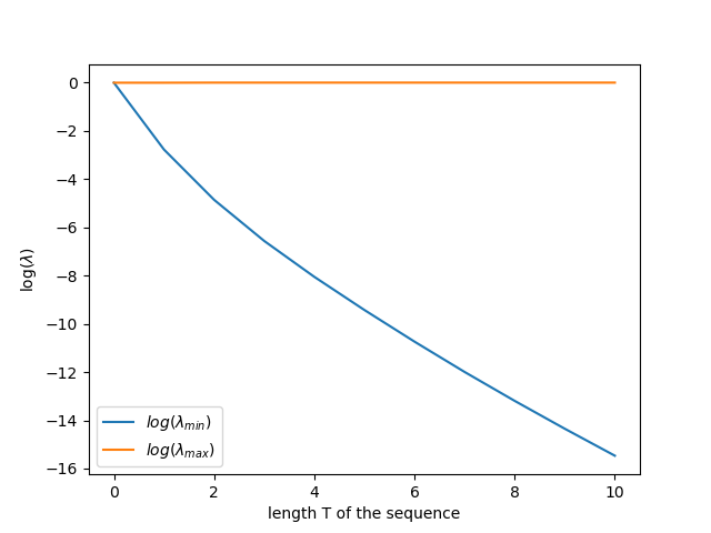
(a) $\rho=0.25$

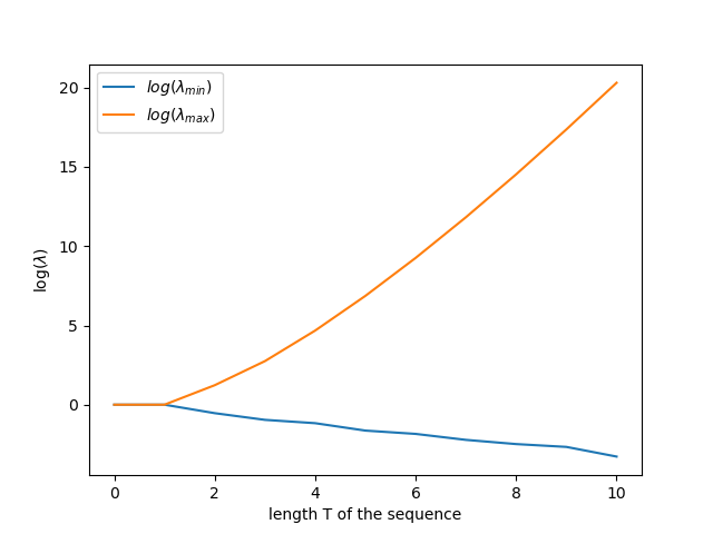
(b) $\rho=1$

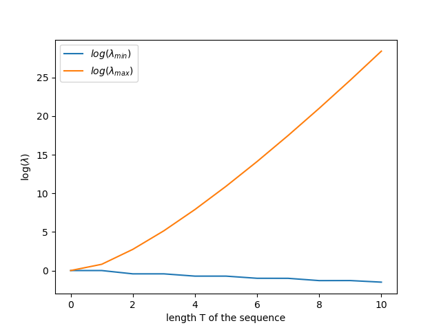
(c) $\rho=1.5$

Figure 1. The evolutions in time of the (logarithms of the) largest and smallest eigenvalues of the Hankel matrix of moments of a Gaussian random variable with standard variation $\rho$.

On the one hand, Theorem 1 highlights the importance of understanding the evolution in time of the smallest eigenvalue $\lambda_{\mathrm{min}}(B_{T})$ of the Hankel matrix of moments $B_{T}$ of the random connectivity of a linear reservoir as a (worst case scenario) theoretical guarantee of (expected) separation of the outputs of very long time series. On the other hand, the plots in Example 2 highlight another equally important problem of a practical nature: understanding the “dominance” of the largest eigenvalue $\lambda_{\mathrm{max}}(B_{T})$ (of $B_{T}$) over $\lambda_{\mathrm{min}}(B_{T})$ or more generally over the rest of the spectrum of $B_{T}$. Indeed, when this dominance is very large, the separation of the outputs is characterised almost fully by a single component; that given by the direction defined by the eigenvector associated to the largest eigenvalue. Combined with the theoretical guarantee $\lambda_{\mathrm{min}}(B_{T})>0$ (and the difficulty of obtaining sharp estimates for $\lambda_{\mathrm{min}}(B_{T})$ in the higher dimensional case), it is this latter point of view of dominance that will dictate the line of reasoning in the rest of the paper: we will estimate the dominance ratio

(4) $$r_{T}=\frac{\lambda_{\mathrm{max}}(B_{T})}{\sum_{i=0}^{T}\lambda_{i}(B_{T})},$$

when $T\to\infty$, where

$$(\lambda_{\mathrm{min}}(B_{T})=)\lambda_{T}(B_{T})\leq\lambda_{T-1}(B_{T})\leq\cdots\leq\lambda_{0}(B_{T})(=\lambda_{\mathrm{max}}(B_{T}))$$

denote the eigenvalues of $B_{T}$. We will see in the rest of the paper that in cases where $r_{T}$ is close to $1$, we will also get suitable equivalents for $\lambda_{\mathrm{max}}(B_{T})$. Figure 2 shows the evolution of the dominance ratio $r_{T}$ in the case of a Gaussian distribution.

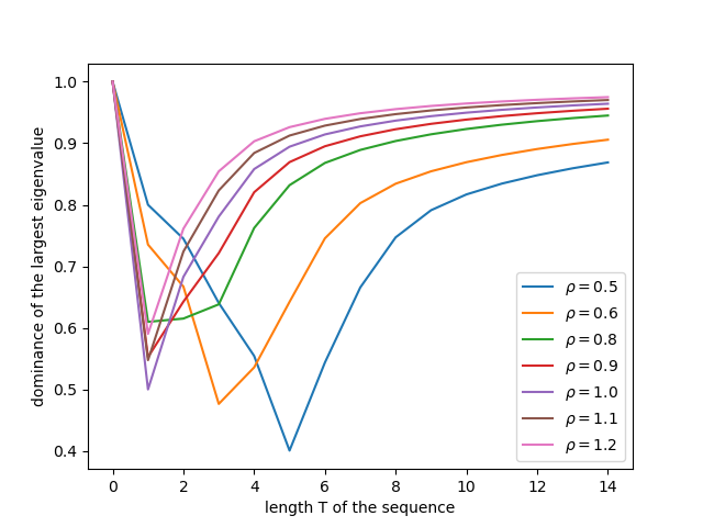
Figure 2. The dominance of the largest eigenvalue over the entire spectrum (as defined in (4)), in function of the length $T$, of the Hankel matrix of moments $B_{T}$ of a centred Gaussian random variable with variance $\rho^{2}$.

Remark 3.

Cauchy’s interlacing theorem (e.g. [Hwa04]) highlights an interlacing phenomena in the eigenvalues of $B_{T}$ as $T$ grows larger. More explicitly, one has

$$\lambda_{T+1}(B_{T+1})\leq\lambda_{T}(B_{T})\leq\lambda_{T}(B_{T+1})\leq\cdots\leq\lambda_{0}(B_{T})\leq\lambda_{0}(B_{T+1}).$$

However, the above does not provide a quantitative estimate on the distances between these eigenvalues or information on the dominance of the largest eigenvalues.

In the following proposition, we give some generic theoretical guarantees on the values of the largest and smallest eigenvalues of $B_{T}$. While these might seem “naive”, they have the advantages of being dimension-free and easy to compute. Moreover, we will see later that these will be enough to give us some idea about the evolution of the values of the largest and smallest eigenvalues of $B_{T}$, and even capture the order of magnitude of the largest eigenvalue in many classical examples.

Proposition 4.

Let $T\in\mathbb{N}^{*}$ and $w$ be a real-valued random variable. Let us denote the moments $m_{t}:=\mathbb{E}w^{t}$, for all $t\in\mathbb{N}$, and define the square Hankel matrix of moments

$$B_{T}:=(m_{i+j})_{0\leq i,j\leq T},$$

with largest eigenvalue (respectively smallest eigenvalue) denoted $\lambda_{\mathrm{max}}(B_{T})$ (resp. $\lambda_{\mathrm{min}}(B_{T})$). Then $(\lambda_{\mathrm{max}}(B_{T}))_{T\geq 1}$ (resp. $(\lambda_{\mathrm{min}}(B_{T}))_{T\geq 1}$) is an increasing (resp. decreasing) sequence. Moreover,

(5) $$\max_{0\leq i\leq T}\sqrt{\sum_{j=0}^{T}m_{i+j}^{2}}\leq\lambda_{\mathrm{max}}(B_{T})\leq\sum_{t=0}^{T}m_{2t},$$

and

$$\lambda_{\mathrm{min}}(B_{T})\leq\min(1,m_{2},\ldots,m_{2T}).$$

Proof.

The monotonicity of the sequences $(\lambda_{\mathrm{max}}(B_{T}))_{T\geq 1}$ and $(\lambda_{\mathrm{min}}(B_{T}))_{T\geq 1}$ can be obtained for example using Cauchy’s interlacing theorem (c.f. Remark 3). Since the eigenvalues of $B_{T}$ are positive and sum up to $\mathrm{tr}(B_{T})$, then

$$\lambda_{\mathrm{max}}(B_{T})\leq\mathrm{tr}(B_{T})=\sum_{t=0}^{T}m_{2t}.$$

One also has (the operator norm of any matrix is larger than the Euclidean norms of its rows)

$$\lambda_{\mathrm{max}}(B_{T})=\left\|B_{T}\right\|_{\mathrm{op}}\geq\|B_{T}\|_{2,\infty}=\max_{0\leq i\leq T}\sqrt{\sum_{j=0}^{T}m_{i+j}^{2}}.$$

Since $B_{T}$ is symmetric, then

$$\lambda_{\mathrm{min}}(B_{T})=\min_{x\neq 0}\frac{x^{\top}B_{T}x}{\|x\|_{2}^{2}}.$$

In the above, taking $x$ to be a basis element in $\mathbb{R}^{T+1}$, we get

$$\lambda_{\mathrm{min}}(B_{T})\leq\min(1,m_{2},\ldots,m_{2T}).$$

∎

Proposition 4 provides us with an easily computable lower bound on the dominance of the largest eigenvalue of $B_{T}$ over its spectrum. More explicitly, one has

$$\widetilde{r}_{T}:=\max_{0\leq i\leq T}\frac{\sqrt{\sum_{j=0}^{T}m_{i+j}^{2}}}{\sum_{t=0}^{T}m_{2t}}\leq r_{T}=\frac{\lambda_{\mathrm{max}}(B_{T})}{\sum_{i=0}^{T}\lambda_{i}(B_{T})}\leq 1.$$

In the cases that interest us in the rest of this paper, i.e. when the entries of the connectivity matrix are Gaussian, we will explicitly show that the above bound becomes sharp in several cases when either the length of the time series or the dimension of the reservoir is very large. However, this is not the case for all distributions; for instance in the one-dimensional case when $w$ is uniformly distributed over the unit interval and $T\to+\infty$.

Theorem 5.

Let $\rho>0$ and $w\sim\mathcal{N}(0,\rho^{2})$. For all $t\in\mathbb{N}$, let us denote its moments $m_{t}:=\mathbb{E}w^{t}$. For $T\in\mathbb{N}^{*}$, define the square Hankel matrix

$$B_{T}:=(m_{i+j})_{0\leq i,j\leq T},$$

with eigenvalues denoted

$$(\lambda_{\mathrm{min}}(B_{T})=)\lambda_{T}(B_{T})\leq\lambda_{T-1}(B_{T})\leq\cdots\leq\lambda_{0}(B_{T})(=\lambda_{\mathrm{max}}(B_{T})).$$

Then, as $T\to\infty$, the largest eigenvalue $\lambda_{\mathrm{max}}(B_{T})$ dominates the spectrum of $B_{T}$, i.e.

$$\frac{\lambda_{\mathrm{max}}(B_{T})}{\sum\limits_{t=0}^{T}\lambda_{i}(B_{T})}\underset{T\to\infty}{\longrightarrow}1.$$

We have furthermore

$$\lambda_{\mathrm{max}}(B_{T})\underset{T\to+\infty}{\simeq}\sqrt{2}\left(\frac{2\rho^{2}T}{e}\right)^{T}\quad\text{and}\quad\lambda_{\mathrm{min}}(B_{T})\underset{T\to+\infty}{\simeq}\frac{2^{5/2}\pi T^{1/4}}{\rho^{3/2}}\exp\left(\frac{1}{2\rho^{2}}-\frac{2\sqrt{T}}{\rho}\right).$$

Proof.

Recall that, for $t\in\mathbb{N}$

$$m_{2t}=\rho^{2t}\frac{(2t)!}{2^{t}t!}=\frac{(2\rho^{2})^{t}}{\sqrt{\pi}}\Gamma\left(t+\frac{1}{2}\right),$$

where $\Gamma$ is the Gamma function. Define the following function for positive real numbers

$$g(t)=(2\rho^{2})^{t}\Gamma\left(t+\frac{1}{2}\right).$$

Let us note that $g$ diverges to $+\infty$ at $+\infty$. One has for $t>0$

$$g^{\prime}(t)=(2\rho^{2})^{t}\Gamma\left(t+\frac{1}{2}\right)\left(\psi^{(0)}\left(t+\frac{1}{2}\right)+\log(2\rho^{2})\right),$$

where $\psi^{(0)}(x):=\frac{\Gamma^{\prime}(x)}{\Gamma(x)}$ is the digamma function (also called polygamma function of order 0). As $\psi^{(0)}$ is strictly increasing on $(0,+\infty)$ and converges to $+\infty$ at $+\infty$, then there exists $t_{1}>0$ (depending on $\rho$) such that $g$ is strictly increasing on $[t_{1},+\infty)$. Let $t_{2}\geq t_{1}$ such that

$$\max_{[0,t_{1}]}g(t)\leq g(t_{2}).$$

Finally, define $t_{0}=\lfloor t_{2}\rfloor+1$. We have then

$$\forall t\leq t_{0}\colon\quad g(t)\leq g(t_{0})\quad\text{and}\quad m_{2t}\leq m_{2t_{0}},$$

and

$$\forall t\geq s\geq t_{0}\colon\quad g(s)\leq g(t)\quad\text{and}\quad m_{2s}\leq m_{2t}.$$

We have then, for $T\geq t_{0}+2$

$$m_{2T}\leq\mathrm{tr}(B_{T})\leq m_{2T}+m_{2(T-1)}+(T-1)m_{2(T-2)}.$$

Hence

$$1\leq\frac{\mathrm{tr}(B_{T})}{m_{2T}}\leq 1+\frac{1}{\rho^{2}(2T-1)}+\frac{T-1}{\rho^{4}(2T-1)(2T-3)},$$

and $\lim\limits_{T\to\infty}\frac{\mathrm{tr}(B_{T})}{m_{2T}}=1$. As a direct consequence of Proposition 4, one has, for all $T\in\mathbb{N}$

$$1\leq\frac{\lambda_{\mathrm{max}}(B_{T})}{m_{2T}}\leq\frac{\mathrm{tr}(B_{T})}{m_{2T}}.$$

Therefore, one also has $\lim\limits_{T\to\infty}\frac{\lambda_{\mathrm{max}}(B_{T})}{m_{2T}}=1$. Thus

$$\frac{\lambda_{\mathrm{max}}(B_{T})}{\sum\limits_{t=0}^{T}\lambda_{i}(B_{T})}=\frac{\lambda_{\mathrm{max}}(B_{T})}{\mathrm{tr}(B_{T})}\underset{T\to\infty}{\longrightarrow}1.$$

We also get (using Stirling’s formula)

$$\lambda_{\mathrm{max}}(B_{T})\underset{T\to+\infty}{\simeq}m_{2T}\underset{T\to+\infty}{\simeq}\sqrt{2}\left(\frac{2\rho^{2}T}{e}\right)^{T}.$$

The techniques to derive an equivalent for $\lambda_{\mathrm{min}}(B_{T})$ are classical in the literature on Hankel matrices of moments, e.g. [Sze36, BCI02, BS11]. Due to its complexity, and in order to keep this proof short, we only recall some of its elements, following the exposition in [Sze36]. $f(\mathbf{a},\cdot)$ being a polynomial, one has

$$\lambda_{\mathrm{min}}(B_{T})=\min_{\mathbf{a}\neq 0}\frac{\mathbb{E}f(\mathbf{a},w)^{2}}{\|\mathbf{a}\|_{2}^{2}}=\min_{\mathbf{a}\neq 0}\frac{\mathbb{E}f(\mathbf{a},w)^{2}}{\frac{1}{2\pi}\int_{0}^{2\pi}|f(\mathbf{a},e^{i\theta})|^{2}\mathrm{d}\theta}.$$

In other words

(6) $$\frac{2\pi}{\lambda_{\mathrm{min}}(B_{T})}=\max_{\mathbf{a}\neq 0}\frac{\int_{0}^{2\pi}|f(\mathbf{a},e^{i\theta})|^{2}\mathrm{d}\theta}{\mathbb{E}f(\mathbf{a},w)^{2}}.$$

Let $(h_{n})_{n\geq 0}$ be the sequence of normalised Hermite polynomials associated to the weight function $e^{-t^{2}}$. Writing $g_{\mathbf{a}}:u\mapsto f({\mathbf{a}},\sqrt{2}\rho u)$ as a linear combination of $\{h_{n},n\in[\![0,T]\!]\}$

$$g_{\mathbf{a}}(u)=\sum_{n=0}^{T}b_{n}h_{n}(u),\quad\text{for all }u\in\mathbb{R},$$

we get, on the one hand

$$\mathbb{E}f({\mathbf{a}},w)^{2}=\frac{1}{\sqrt{\pi}}\int_{-\infty}^{+\infty}g_{\mathbf{a}}^{2}(t)e^{-t^{2}}\mathrm{d}t=\frac{1}{\sqrt{\pi}}\int_{-\infty}^{+\infty}\left(\sum_{n=0}^{T}b_{n}h_{n}(t)\right)^{2}e^{-t^{2}}\mathrm{d}t=\frac{\|\mathbf{b}\|_{2}^{2}}{\sqrt{\pi}}.$$

On the other hand

$$\begin{array}[]{rcl}\int_{0}^{2\pi}|f(\mathbf{a},e^{i\theta})|^{2}\mathrm{d}\theta&=&\int_{0}^{2\pi}g_{\mathbf{a}}\left(\frac{e^{i\theta}}{\sqrt{2}\rho}\right)\overline{g_{\mathbf{a}}\left(\frac{e^{i\theta}}{\sqrt{2}\rho}\right)}\mathrm{d}\theta\\ &=&\sum\limits_{0\leq n,m\leq T}b_{n}b_{m}\int_{0}^{2\pi}h_{n}\left(\frac{e^{i\theta}}{\sqrt{2}\rho}\right)\overline{h_{m}\left(\frac{e^{i\theta}}{\sqrt{2}\rho}\right)}\mathrm{d}\theta.\\ \end{array}$$

Defining

(7) $$R_{n,m}=\int_{0}^{2\pi}h_{n}\left(\frac{e^{i\theta}}{\sqrt{2}\rho}\right)\overline{h_{m}\left(\frac{e^{i\theta}}{\sqrt{2}\rho}\right)}\mathrm{d}\theta,$$

for all $n,m\in\mathbb{N}$, we get

$$\frac{2\sqrt{\pi}}{\lambda_{\mathrm{min}}(B_{T})}=\max_{\mathbf{b}\in\mathbb{S}^{T}}\sum_{0\leq n,m\leq T}b_{n}b_{m}R_{n,m},$$

where $\mathbb{S}^{T}$ denotes the unit sphere in $\mathbb{R}^{T+1}$. From here, the proof and the computations are exactly as in [Sze36], to which we will strongly refer. First, it is easy to check that $R_{n,m}>0$ if $n+m$ is even. By expressing the Hermite polynomials in terms of the (generalised) Laguerre polynomials, one further shows that $R_{n,m}=0$ if $n+m$ is odd [Sze36, Part IV]. Using the asymptotic formula (for large $n$) of Laguerre polynomials, one then argues [Sze36, Part II] that the essential part of $R_{n,m}$ (for large $n$ and $m$) is obtained by the value of the integral (7) along small arcs around the imaginary axis. This gives the following estimate for large $n$ and $m$ being of the same order of magnitude $T$ (up to an additive $\sqrt{T}$ factor) and such that $n+m$ is even [Sze36, Part IV, Eq. (38)]

$$R_{n,m}\simeq\frac{\sqrt{2\rho}}{2\sqrt{\pi}T^{3/4}}\exp\left(-\frac{1}{2\rho^{2}}\right)\exp\left(\frac{\sqrt{n}+\sqrt{m}}{\rho}\right).$$

Next, it is argued [Sze36, Part II.3] using the Cauchy-Schwarz inequality that, for large $T$, the maximum in (6) is essentially obtained as a sum of the $R_{n,n}$, where $n$ is of the same magnitude as $T$ (up to an additive $\sqrt{T}$ factor). Finally, an estimate of this sum via an integral gives

$$\frac{2\sqrt{\pi}}{\lambda_{\mathrm{min}}(B_{T})}\simeq\frac{2^{-3/2}\rho^{3/2}}{\sqrt{\pi}T^{1/4}}\exp\left(-\frac{1}{2\rho^{2}}\right)\exp\left(\frac{2\sqrt{T}}{\rho}\right),$$

which directly yields the estimate in the statement of the theorem (and corresponds to the expression in [Sze36, Eq. 11] when $\rho$ is replaced by $\frac{1}{\sqrt{2}}$.) ∎

Let us summarise the consequences of Theorem 5 in terms of the expected separation capacity of the one-dimensional random linear reservoir with Gaussian connectivity $w$:

• No matter the value of the standard deviation $\rho$ of $w$, which we may think of as a hyperparameter of the architecture, the largest eigenvalue $\lambda_{\mathrm{max}}(B_{T})$ grows super-exponentially fast as the length $T$ of the time series grows larger. In contrast, the smallest eigenvalue $\lambda_{\mathrm{min}}(B_{T})$ decays slightly less than exponentially fast. As illustrated by Figure 1, a choice of a larger $\rho$ can marginally slow this decay.

• No matter the value of the standard deviation $\rho$ of $w$, the largest eigenvalue $\lambda_{\mathrm{max}}(B_{T})$ dominates the spectrum of $B_{T}$ as $T\to\infty$. Hence, for large $T$, the expected separation of two time series by the random reservoir is almost entirely influenced by their coordinates along the direction of the largest eigenvalue of $B_{T}$. As illustrated by Figure 2 (and by the proof of Theorem 5, assuming the sharpness of the bound (5)), this dominance can be slightly delayed in time by a choice of a smaller hyperparameter $\rho$.

In light of the above remarks, and following Theorem 1, the expected separation capacity of the (Gaussian) reservoir is bound to deteriorate for long time series. When choosing the hyperparameter $\rho$, there is a trade-off phenomenon between the non-dominance of a single direction (through the ratio $r_{T}$) and a guarantee of separation for all time series (through $\lambda_{\mathrm{min}}(B_{T})$).

3.2. The higher-dimensional case

In this subsection, we will generalise some of the previous results. We will furthermore analyse the effects on the separation capacity by time, reservoir dimension, generating distribution of the connectivity matrix and any symmetry assumptions thereon.

We recall that the final hidden state of the $N$-dimensional reservoir with pre-processing matrix $u$ and connectivity matrix $W$ is given by

$$f(\mathbf{a},W)=\sum_{t=0}^{T}W^{t}ua_{T-t}=(f_{i})_{1\leq i\leq N}\in\mathbb{R}^{N}.$$

As argued in Section 2, we will take $u=(1,1,\ldots,1)^{\top}\in\mathbb{R}^{N}$. Let us first generalise the result from Theorem 1 and show that the reservoir separation capacity is characterised by the spectral analysis of a generalised matrix of moments.

Theorem 6.

Consider an $N$-dimensional linear reservoir with random connectivity matrix $W$, i.e. the output of the reservoir for the signal $\mathbf{x}:=(x_{t})_{0\leq t\leq T}$ is given by

$$f(\mathbf{x},w)=\sum_{t=0}^{T}W^{t}ux_{T-t},$$

where $u=(1,1,\ldots,1)^{\top}$. Then the expected separation capacity of the reservoir is characterised by the eigenvalues of the symmetric positive semi-definite matrix

(8) $$B_{T,N}:=\mathbb{E}\left(\sum_{i=1}^{N}\beta_{i,l_{1}}\beta_{i,l_{2}}\right)_{0\leq l_{1},l_{2}\leq T}\in\mathbb{R}^{(T+1)\times(T+1)},$$

where, for $i\in[\![1,N]\!]$

$$\beta_{i,0}=1\quad\text{and}\quad\beta_{i,l}=\sum_{i_{1},i_{2},\ldots,i_{l}=1}^{N}W_{ii_{1}}W_{i_{1}i_{2}}\cdots W_{i_{l-1}i_{l}}.$$

More specifically, if $\lambda_{\mathrm{min}}(B_{T,N})$ and $\lambda_{\mathrm{max}}(B_{T,N})$ denote respectively the smallest and largest eigenvalue of $B_{T,N}$ and given two time series $\mathbf{x}$ and $\mathbf{y}$, one has

(9) $$\lambda_{\mathrm{min}}(B_{T,N})\|\mathbf{x}-\mathbf{y}\|^{2}_{2}\leq\mathbb{E}\|f(\mathbf{x},W)-f(\mathbf{y},W)\|^{2}_{2}\leq\lambda_{\mathrm{max}}(B_{T,N})\|\mathbf{x}-\mathbf{y}\|^{2}_{2}.$$

Proof.

Given two time series $\mathbf{x}$ and $\mathbf{y}$, and defining $\mathbf{a}:=\mathbf{x}-\mathbf{y}$, we get $f(\mathbf{x},W)-f(\mathbf{y},W)=f(\mathbf{a},W)$. Denoting $f(\mathbf{a},W)=(f_{i})_{1\leq i\leq N}\in\mathbb{R}^{N}$, then, for all $i\in[\![1,N]\!]$

$$f_{i}=a_{T}+\left(\sum\limits_{j=1}^{N}W_{ij}\right)a_{T-1}+\cdots+\left(\sum\limits_{i_{1},i_{2},\ldots,i_{T}=1}^{N}W_{ii_{1}}W_{i_{1}i_{2}}\cdots W_{i_{T-1}i_{T}}\right)a_{0}=\sum\limits_{l=0}^{T}a_{T-l}\beta_{i,l}.$$

Hence

$$\|f(\mathbf{a},W)\|^{2}_{2}=\sum_{i=1}^{N}f_{i}^{2}=\sum_{i=1}^{N}\left(\sum_{l=0}^{T}a_{T-l}\beta_{i,l}\right)^{2}=\sum_{l_{1},l_{2}=0}^{T}a_{T-l_{1}}a_{T-l_{2}}\left(\sum_{i=1}^{N}\beta_{i,l_{1}}\beta_{i,l_{2}}\right).$$

Therefore $\mathbb{E}\|f(\mathbf{a},W)\|^{2}_{2}=a^{\top}B_{T,N}a$, where $a=(a_{T},\ldots,a_{0})^{\top}$, which then yields inequality (9). ∎

Similarly to the 1-dimensional case, the spectral analysis of $B_{T,N}$ provides an orthonormal basis of $\mathbb{R}^{T+1}$ that explains the quality of (expected) separation of the outputs of two time series by the random reservoir. In view of its importance in the rest of this subsection, let us fix the definition of $B_{T,N}$.

Definition 7.

Let $W\in\mathbb{R}^{N\times N}$ be a random matrix and $T\in\mathbb{N}^{*}$. We call the generalised matrix of moments of $W$ of order $T$ the matrix denoted $B_{T,N}$ that is defined by

$$B_{T,N}=(B_{T,N}(l_{1},l_{2}))_{0\leq l_{1},l_{2}\leq T}:=\mathbb{E}\left(\sum_{i=1}^{N}\beta_{i,l_{1}}\beta_{i,l_{2}}\right)_{0\leq l_{1},l_{2}\leq T}\in\mathbb{R}^{(T+1)\times(T+1)},$$

where, for $i\in[\![1,N]\!]$, $\beta_{i,0}=1$ and

$$\beta_{i,l}=\sum_{i_{1},i_{2},\ldots,i_{l}=1}^{N}W_{ii_{1}}W_{i_{1}i_{2}}\cdots W_{i_{l-1}i_{l}}.$$

Note that, in contrast to the one-dimensional case, $B_{T,N}$ is not always a Hankel matrix. For instance, if $W\in\mathbb{R}^{2\times 2}$ has i.i.d. standard Gaussian entries, then it is easy to check that $B_{2,2}(0,2)\neq B_{2,2}(1,1)$.

Similarly to the one-dimensional case (Proposition 2), it is clear that if $W$ is supported in a set with non-empty interior then $B_{T,N}$ is positive definite and thus, separation is guaranteed in expectation. Moreover, there is an interlacing phenomenon between the eigenvalues of $B_{T,N}$ and $B_{T+1,N}$ (as observed in Remark 3.)

Generalising Proposition 4, which is actually valid for any symmetric positive semi-definite matrix, gives the following bounds.

Proposition 8.

Let $N\in\mathbb{N}^{*}$ and $W\in\mathbb{R}^{N\times N}$ be a random matrix. For every $T\in\mathbb{N}^{*}$ , let $B_{T,N}$ denote the generalised matrix of moments of $W$ as given in Definition 7 and denote its largest eigenvalue by $\lambda_{\mathrm{max}}(B_{T,N})$. Then $(\lambda_{\mathrm{max}}(B_{T,N}))_{T\geq 1}$ is an increasing sequence. Moreover,

(10) $$\max\limits_{0\leq l_{1}\leq T}\sqrt{\sum\limits_{l_{2}=0}^{T}\left(B_{T,N}(l_{1},l_{2})\right)^{2}}\leq\lambda_{\mathrm{max}}(B_{T,N})\leq\mathrm{tr}(B_{T,N})=\sum_{l=0}^{T}B_{T,N}(l,l).$$

Proof.

Similar to Proposition 4. ∎

In the proposition above, we have omitted the bounds on the smallest eigenvalues as the methods described in the previous subsection are hard to generalise in higher dimensions. In this section, we will restrict ourselves then to understanding, on the one hand, the best-case-scenario separation capacity of the reservoir given by $\lambda_{\mathrm{max}}(B_{T,N})$, and on the other hand, the quality of this separation expressed by the dominance of the largest eigenvalue $\lambda_{\mathrm{max}}(B_{T,N})$ over the full spectrum of $B_{T,N}$, i.e. the dominance ratio

(11) $$r_{T,N}:=\frac{\lambda_{\mathrm{max}}(B_{T,N})}{\sum\limits_{i=0}^{T}\lambda_{i}(B_{T,N})}.$$

Assuming sharpness of inequality (10), the bounds in Proposition 8 highlight the importance of understanding the order of the terms $B_{T,N}(l_{1},l_{2})$ for $l_{1},l_{2}\in[\![0,T]\!]$, for $T$ or $N$ large. The methodology for the computations of such orders (especially for large $N$) are very classical in the literature of random matrices (e.g. [AGZ10]). To simplify the computations but also to be in line with the common practical implementation of reservoirs, we will restrict ourselves in the remaining of this paper to connectivity matrices with Gaussian entries. Nevertheless, most computations generalise easily to other cases. We will in particular distinguish two cases that are common in practice, one where the connectivity matrix $W$ is assumed to be symmetric and one where all of its entries are assumed to be independent. The (random) entries of the connectivity matrix are usually chosen to have a standard deviation equal to $\frac{\rho}{\sqrt{N}}$, with $\rho$ close to $1$, and $N$ very large. For the purpose of understanding the advantage of such a choice (beyond numerical stability and easiness of interpretation), we will consider a more general class of standard deviations of the type $\frac{\rho}{N^{\alpha}}$, with $\alpha\geq 0$. Before we carry on, we will need a compact notation for the Gaussian moments.

Notation 9.

Given a standard Gaussian random variable $X$, we denote its moments by

$$\forall t\in\mathbb{N}:\quad m_{t}:=\mathbb{E}X^{t}.$$

Trivially, for all $t,s\in\mathbb{N}$, one has $m_{t}m_{s}\leq m_{t+s}$. Let us also introduce the following multi-index notation.

Notation 10.

Given a matrix $W\in\mathbb{R}^{N\times N}$, $l\geq 2$ and $\mathbf{i}=(i_{1},i_{2},\ldots,i_{l})\in[N]^{l}$, we denote

$$W_{\mathbf{i}}:=W_{i_{1}i_{2}}W_{i_{2}i_{3}}\cdots W_{i_{l-1}i_{l}}.$$

3.2.1. The symmetric case

We start with the symmetric case which is the most readily available in the literature of random matrices as the computation of moments similar to those appearing in Definition 7 and inequality (10) lead to the celebrated Wigner semi-circle law ([Wig55, AGZ10]). Before we start these computations, let us introduce the following graph-theoretic definition.

Definition 11.

Given a non-directed graph $G$ (with possibly self-edges), a sequence

$$w=(v_{1},v_{2},\ldots,v_{l})$$

is called a walk on the graph $G$ of length $l-1$ if the following two conditions are satisfied:

• For all $i\in[l]$, $v_{i}$ is a vertex in $G$,

• For all $i\in[l-1]$, $\{v_{i},v_{i+1}\}$ is an edge in $G$.

If $v_{l}=v_{1}$, we say that $w$ is a loop (on $G$).

We denote the sets of vertices and edges of any graph $G$ by $V_{G}$ and $E_{G}$ respectively. Recall that by Euler’s formula ([Bol13]), $|V_{G}|-|E_{G}|\leq 1$, with equality if and only if $G$ is a tree. Let us now move to our main estimate.

Lemma 12.

Let $N,T\in\mathbb{N}^{*}$, $\rho>0$ and $\alpha\in\mathbb{R}$. Let $W$ be a symmetric $N\times N$ random matrix such that its entries on and above the diagonal are i.i.d. centred Gaussian random variables with standard deviation $\frac{\rho}{N^{\alpha}}$. Denote by $B_{T,N}$ its generalised matrix of moments of order $T$ as given in Definition 7. For $l_{1},l_{2}\in[\![0,T]\!]$, we have the following.

• If $l_{1}+l_{2}$ is odd, then $B_{T,N}(l_{1},l_{2})=0$.

• If $l_{1}+l_{2}$ is even and $\frac{l_{1}+l_{2}}{2}+1\leq N$, then

  $$\begin{array}[]{lcl}\frac{\rho^{l_{1}+l_{2}}}{\frac{l_{1}+l_{2}}{2}+1}{l_{1}+l_{2}\choose\frac{l_{1}+l_{2}}{2}}\frac{N(N-1)\cdots(N-\frac{l_{1}+l_{2}}{2})}{N^{\alpha(l_{1}+l_{2})}}&\leq&B_{T,N}(l_{1},l_{2})\\ &\leq&\frac{\rho^{l_{1}+l_{2}}}{\frac{l_{1}+l_{2}}{2}+1}{l_{1}+l_{2}\choose\frac{l_{1}+l_{2}}{2}}N^{(l_{1}+l_{2})\left(\frac{1}{2}-\alpha\right)+1}\\ &&+\rho^{l_{1}+l_{2}}m_{l_{1}+l_{2}}\left(\frac{l_{1}+l_{2}}{2}\right)^{l_{1}+l_{2}}N^{(l_{1}+l_{2})\left(\frac{1}{2}-\alpha\right)}.\\ \end{array}$$

Proof.

Let $l_{1},l_{2}\in[\![0,T]\!]$. Recall the definition

$$B_{T,N}(l_{1},l_{2})=\mathbb{E}\sum\limits_{\begin{subarray}{c}1\leq i,i_{1},\ldots,i_{l_{1}}\leq N\\ 1\leq j_{1},\ldots,j_{l_{2}}\leq N\end{subarray}}W_{ii_{1}}W_{i_{1}i_{2}}\cdots W_{i_{l_{1}-1}i_{l_{1}}}W_{ij_{1}}W_{j_{1}j_{2}}\cdots W_{j_{l_{2}-1}j_{l_{2}}}.$$

As the odd moments of a centred Gaussian distribution are all null, the above expression shows that indeed $B_{T,N}(l_{1},l_{2})=0$ if $l_{1}+l_{2}$ is odd. Assume now that $l_{1}+l_{2}$ is even. Using the symmetry of $W$, one gets

(12) $$B_{T,N}(l_{1},l_{2})=\mathbb{E}\sum_{\begin{subarray}{c}1\leq i,i_{1},\ldots,i_{l_{1}}\leq N\\ 1\leq j_{1},\ldots,j_{l_{2}}\leq N\end{subarray}}W_{j_{l_{2}}j_{l_{2}-1}}\cdots W_{j_{2}j_{1}}W_{j_{1}i}W_{ii_{1}}W_{i_{1}i_{2}}\cdots W_{i_{l_{1}-1}i_{l_{1}}}=\mathbb{E}\sum_{\mathbf{i}\in[N]^{l_{1}+l_{2}+1}}W_{\mathbf{i}}.$$

Let $\mathbf{i}=(i_{1},i_{2},\ldots,i_{l_{1}+l_{2}+1})\in[N]^{l_{1}+l_{2}+1}$. Define a mapping $g_{\mathbf{i}}:\{i_{1},i_{2},\ldots,i_{l_{1}+l_{2}+1}\}\to\mathbb{N}^{*}$ by the recursive relation

• $g_{\mathbf{i}}(i_{1})=1$,

• for $k\in[\![2,l_{1}+l_{2}+1]\!]$, if there exists $p<k$ such that $i_{k}=i_{p}$ then $g_{\mathbf{i}}(i_{k})=g_{\mathbf{i}}(i_{p})$, otherwise $g_{\mathbf{i}}(i_{k})=g_{\mathbf{i}}(i_{k-1})+1$.

This way, we see that $\mathbf{i}$ defines a unique pair $(G,w)$, where

• $G$ is a connected graph whose vertices are given by the set

  $$\{g_{\mathbf{i}}(i_{1}),g_{\mathbf{i}}(i_{2}),\ldots,g_{\mathbf{i}}(i_{l_{1}+l_{2}+1})\},$$

  and whose only edges are the ones connecting $g_{\mathbf{i}}(i_{k})$ to $g_{\mathbf{i}}(i_{k+1})$, for $k\in[l_{1}+l_{2}]$. Note that $G$ has at most $\min(l_{1}+l_{2}+1,N)$ vertices.

• $w=(g_{\mathbf{i}}(i_{1}),g_{\mathbf{i}}(i_{2}),\ldots,g_{\mathbf{i}}(i_{l_{1}+l_{2}+1}))$ is a walk on $G$ of length $l_{1}+l_{2}$ crossing all the edges of $G$. Moreover, given any two vertices $m$ and $n$ in $G$, if $m<n$ then $w$ visits the vertex $m$ for the first time before it visits the vertex $n$.

For instance, if $\mathbf{i}=(1,2,3,3,2,5,7)$ then the vertices of $G$ are $\{1,2,3,4,5\}$ and its edges are given by

$$\{1,2\},\{2,3\},\{3\},\{2,4\},\{4,5\},$$

while

$$w=(1,2,3,3,2,4,5).$$

In such cases let us write $\mathbf{i}\sim(G,w)$. Note that this construction is not one-to-one. Given such a pairing $(G,w)$, where $w$ is of length $L$, we can recover all the $(L+1)$-tuples that are mapped to it by injectively mapping the vertices of $G$ to elements in $[N]$. Let us denote the set of all pairings $(G,w)$ obtained in this manner by $\mathcal{G}_{N,l_{1}+l_{2}}$.

Next, we note that, for $\mathbf{i}\in[N]^{l_{1}+l_{2}+1}$, the quantity $\mathbb{E}W_{\mathbf{i}}$ depends only on the pair graph-walk $(G,w)$ mapped to it: different $(l_{1}+l_{2}+1)$-tuples $\mathbf{i}$ associated to the same pair $(G,w)$ yield the same expectation $\mathbb{E}W_{\mathbf{i}}$. Let us denote this quantity $E(G,w)$ and remark that

(13) $$0\leq E(G,w)\leq\frac{\rho^{l_{1}+l_{2}}}{N^{\alpha(l_{1}+l_{2})}}m_{l_{1}+l_{2}}.$$

In summary, we have then

(14) $$\begin{array}[]{rcl}B_{T,N}(l_{1},l_{2})&=&\sum\limits_{(G,w)\in\mathcal{G}_{N,l_{1}+l_{2}}}E(G,w)\cdot\left|\left\{\mathbf{i}\in[N]^{l_{1}+l_{2}+1},\;\;\mathbf{i}\sim(G,w)\right\}\right|\\ &=&\sum\limits_{(G,w)\in\mathcal{G}_{N,l_{1}+l_{2}}}E(G,w)N(N-1)\cdots(N-|V_{G}|+1),\\ \end{array}$$

with all the terms in the above sum being positive. For $(G,w)\in\mathcal{G}_{N,l_{1}+l_{2}}$, and because all the odd moments of centred Gaussian random variables are equal to $0$, we note that $E(G,w)\neq 0$ if and only if $w$ visits each edge of $G$ an even number of times. We will only consider such pairings in the remainder of this proof. In this case, $w$ is necessarily a loop, $|E_{G}|\leq\frac{l_{1}+l_{2}}{2}$ (as each edge of $G$ is visited at least twice by $w$) and $|V_{G}|\leq\frac{l_{1}+l_{2}}{2}+1$ (by Euler’s formula). Let us separate two cases.

Case 1: $|V_{G}|=\frac{l_{1}+l_{2}}{2}+1$. Note that this case occurs only if $\frac{l_{1}+l_{2}}{2}+1\leq N$. This implies in particular that $|E_{G}|=\frac{l_{1}+l_{2}}{2}$ (by Euler’s formula). Hence $G$ is a tree and $w$ is a loop on $G$ visiting each edge exactly twice (otherwise we will have the contradiction $|E_{G}|<\frac{l_{1}+l_{2}}{2}$). The numbers of such pairs $(G,w)$ is classically given by (via an identification with Dyck paths, which themselves are related to the Catalan numbers ([CLRS22, HP91]))

$$\frac{1}{\frac{l_{1}+l_{2}}{2}+1}{l_{1}+l_{2}\choose\frac{l_{1}+l_{2}}{2}}.$$

For such pairs, $E(G,w)$ can be written as the product of second moments of centred Gaussian random variables and is therefore equal to $\frac{\rho^{l_{1}+l_{2}}}{N^{\alpha(l_{1}+l_{2})}}$. By considering only such terms in identity (14), we get then the following lower bound

$$\frac{\rho^{l_{1}+l_{2}}}{\frac{l_{1}+l_{2}}{2}+1}{l_{1}+l_{2}\choose\frac{l_{1}+l_{2}}{2}}\frac{N(N-1)\cdots(N-\frac{l_{1}+l_{2}}{2})}{N^{\alpha(l_{1}+l_{2})}}\leq B_{T,N}(l_{1},l_{2}).$$

Case 2: $|V_{G}|\leq\frac{l_{1}+l_{2}}{2}$. The number of pairings $(G,w)$ satisfying $|V_{G}|\leq\frac{l_{1}+l_{2}}{2}$ is loosely bounded by $\left(\frac{l_{1}+l_{2}}{2}\right)^{l_{1}+l_{2}}$ (i.e. the number of ways to construct a walk (with possible self-edges) on a maximum of $\frac{l_{1}+l_{2}}{2}$ vertices). Using the computation from the previous case (assuming $\frac{l_{1}+l_{2}}{2}+1\leq N$) and the bound (13), we get then

$$\begin{array}[]{rcl}B_{T,N}(l_{1},l_{2})&\leq&\frac{\rho^{l_{1}+l_{2}}}{\frac{l_{1}+l_{2}}{2}+1}{l_{1}+l_{2}\choose\frac{l_{1}+l_{2}}{2}}\frac{N(N-1)\cdots(N-\frac{l_{1}+l_{2}}{2})}{N^{\alpha(l_{1}+l_{2})}}\\ &&+\sum\limits_{\begin{subarray}{c}(G,w)\in\mathcal{G}_{N,l_{1}+l_{2}}\\ |V_{G}|\leq\frac{l_{1}+l_{2}}{2}\end{subarray}}E(G,w)N(N-1)\cdots(N-|V_{G}|+1)\\ &\leq&\frac{\rho^{l_{1}+l_{2}}}{\frac{l_{1}+l_{2}}{2}+1}{l_{1}+l_{2}\choose\frac{l_{1}+l_{2}}{2}}N^{(l_{1}+l_{2})\left(\frac{1}{2}-\alpha\right)+1}+\rho^{l_{1}+l_{2}}m_{l_{1}+l_{2}}\left(\frac{l_{1}+l_{2}}{2}\right)^{l_{1}+l_{2}}N^{(l_{1}+l_{2})\left(\frac{1}{2}-\alpha\right)}.\\ \end{array}$$

The proof is now complete. ∎

Remark 13.

Identity (12) shows that $B_{T,N}$ is indeed a Hankel matrix in this (symmetric) case.

We are now able to quantify the effect of large dimensions on the separation capacity of a reservoir with symmetric Gaussian connectivity matrix.

Theorem 14.

Let $T\in\mathbb{N}^{*}$, $\rho>0$, $\alpha\in\mathbb{R}$. For $N\in\mathbb{N}^{*}$, let $W_{N}$ be a symmetric $N\times N$ random matrix such that its entries on and above the diagonal are i.i.d. centred Gaussian random variables with standard deviation $\frac{\rho}{N^{\alpha}}$. Let $B_{T,N}$ be its generalised matrix of moments of order $T$ as given in Definition 7, with eigenvalues denoted

$$(\lambda_{\min}(B_{T,N})=)\lambda_{T}(B_{T,N})\leq\lambda_{T-1}(B_{T,N})\leq\cdots\leq\lambda_{0}(B_{T,N})(=\lambda_{\mathrm{max}}(B_{T,N})).$$

• If $\alpha=1/2$, then

  $$\frac{\lambda_{\max}(B_{T,N})}{N}\underset{N\to+\infty}{\longrightarrow}\lambda_{\max}(A_{\mathrm{sc}}(\rho,T))\quad\text{and}\quad\frac{\lambda_{\min}(B_{T,N})}{N}\underset{N\to+\infty}{\longrightarrow}\lambda_{\min}(A_{\mathrm{sc}}(\rho,T))$$

  where $\lambda_{\max}(A_{\mathrm{sc}}(\rho,T))$ (respectively $\lambda_{\min}(A_{\mathrm{sc}}(\rho,T))$) denotes the largest (resp. the smallest) eigenvalue of $A_{\mathrm{sc}}(\rho,T)=((A_{\mathrm{sc}}(\rho,T))_{l_{1},l_{2}})_{0\leq l_{1},l_{2}\leq T}$, the Hankel matrix of moments of order $T$ of the (rescaled) semi-circle law given by

  $$(A_{\mathrm{sc}}(\rho,T))_{l_{1},l_{2}}=\left\{\begin{array}[]{ll}0&\text{if }l_{1}+l_{2}\text{ is odd,}\\ \frac{\rho^{l_{1}+l_{2}}}{\frac{l_{1}+l_{2}}{2}+1}{l_{1}+l_{2}\choose\frac{l_{1}+l_{2}}{2}}&\text{otherwise.}\\ \end{array}\right.$$

  Moreover

  $$\lim_{N\to\infty}\frac{\lambda_{\max}(B_{T,N})}{\sum\limits_{i=0}^{T}\lambda_{i}(B_{T,N})}=\frac{\lambda_{\max}(A_{\mathrm{sc}}(\rho,T))}{\mathrm{tr}(A_{\mathrm{sc}}(\rho,T))}.$$

• If $\alpha<1/2$, then

  $$\lambda_{\max}(B_{T,N})\underset{N\to+\infty}{\simeq}\frac{\rho^{2T}}{T+1}{2T\choose T}N^{1+2T\left(\frac{1}{2}-\alpha\right)},$$

  and $\lambda_{\max}(B_{T,N})$ dominates the spectrum of $B_{T,N}$ as $N$ goes to infinity, i.e.

  $$\lim_{N\to\infty}\frac{\lambda_{\max}(B_{T,N})}{\sum\limits_{i=i}^{T}\lambda_{0}(B_{T,N})}=1.$$

• If $\alpha>1/2$, then

  $$\lambda_{\max}(B_{T,N})\underset{N\to+\infty}{\simeq}N,$$

  and $\lambda_{\max}(B_{T,N})$ dominates the spectrum of $B_{T,N}$ as $N$ goes to infinity.

Proof.

For large $N$, Lemma 12 implies

$$\begin{array}[]{ll}\sum\limits_{t=0}^{T}\frac{\rho^{2t}}{t+1}{2t\choose t}\frac{N(N-1)\cdots(N-t)}{N^{2\alpha t}}&\leq\sum\limits_{l=0}^{T}B_{T,N}(l,l)\\ &\leq\sum\limits_{t=0}^{T}\left(\rho^{2t}m_{2t}t^{2t}N^{2t\left(\frac{1}{2}-\alpha\right)}+\frac{\rho^{2t}}{t+1}{2t\choose t}N^{1+2t\left(\frac{1}{2}-\alpha\right)}\right).\\ \end{array}$$

Hence

$$\mathrm{tr}(B_{T,N})\underset{N\to+\infty}{\simeq}\sum_{t=0}^{T}\frac{\rho^{2t}}{t+1}{2t\choose t}N^{1+2t\left(\frac{1}{2}-\alpha\right)}.$$

Similarly

$$\|B_{T,N}\|_{2,\infty}\underset{N\to+\infty}{\simeq}\max_{0\leq l_{1}\leq T}\sqrt{\sum\limits_{\begin{subarray}{c}0\leq l_{2}\leq T\\ l_{1}+l_{2}\text{ even}\end{subarray}}\left(\frac{\rho^{l_{1}+l_{2}}}{\frac{l_{1}+l_{2}}{2}+1}{l_{1}+l_{2}\choose\frac{l_{1}+l_{2}}{2}}N^{(l_{1}+l_{2})\left(\frac{1}{2}-\alpha\right)+1}\right)^{2}}.$$

We have the following cases.

Case 1: $\alpha<1/2$. In this case

$$\mathrm{tr}(B_{T,N})\underset{N\to+\infty}{\simeq}B_{T,N}(T,T)\underset{N\to+\infty}{\simeq}\|B_{T,N}\|_{2,\infty}.$$

Therefore

$$\lambda_{\max}(B_{T,N})\underset{N\to+\infty}{\simeq}\frac{\rho^{2T}}{T+1}{2T\choose T}N^{1+2T\left(\frac{1}{2}-\alpha\right)},$$

and $\lambda_{\max}(B_{T,N})$ dominates the spectrum of $B_{T,N}$ as $N$ goes to infinity

$$\lim_{N\to\infty}\frac{\lambda_{\max}(B_{T,N})}{\sum\limits_{i=0}^{T}\lambda_{0}(B_{T,N})}=\lim_{N\to\infty}\frac{\lambda_{\max}(B_{T,N})}{\mathrm{tr}(B_{T,N})}=1.$$

Case 2: $\alpha>1/2$. Similarly

$$\lambda_{\max}(B_{T,N})\underset{N\to+\infty}{\simeq}B_{T,N}(0,0)\underset{N\to+\infty}{\simeq}N,$$

and $\lambda_{\max}(B_{T,N})$ dominates the spectrum of $B_{T,N}$ as $N$ goes to infinity.

Case 3: $\alpha=1/2$. By Lemma 12, for all $l_{1},l_{2}\in[\![0,T-1]\!]$

$$\frac{B_{T,N}(l_{1},l_{2})}{N}\underset{N\to+\infty}{\longrightarrow}(A_{\mathrm{sc}}(\rho,T))_{l_{1},l_{2}}=\left\{\begin{array}[]{ll}0&\text{if }l_{1}+l_{2}\text{ is odd,}\\ \frac{\rho^{l_{1}+l_{2}}}{\frac{l_{1}+l_{2}}{2}+1}{l_{1}+l_{2}\choose\frac{l_{1}+l_{2}}{2}}&\text{otherwise.}\\ \end{array}\right.$$

The claim follows trivially from the above. ∎

Remark 15.

$A_{\mathrm{sc}}(\rho,T)$ corresponds to the Hankel matrix of moments of the rescaled Wigner semi-circle law whose density is given by

$$\frac{1}{2\pi\rho}\sqrt{\max(4\rho-x^{2},0)},\;\;\text{for all }x\in\mathbb{R}.$$

Remark 16.

The extra $N$ factor appearing in Theorem 14 (for example in the limit case for $\alpha=1/2$) is merely due to the norm of the chosen pre-processing matrix $u$. This factor will disappear if we choose $u$ to be, for instance, the unit vector $\frac{1}{\sqrt{N}}(1,\ldots,1)^{\top}$.

The above theorem shows that the effect of increasing the dimension of the reservoir is an increase in the largest eigenvalue of $B_{T,N}$ that is at most polynomial. However, when not properly rescaled (i.e. $\alpha\neq 1/2$), increasing the dimension of the reservoir has the undesired effect of having the separation property of the reservoir being completely determined by a single direction (in the space of time series $\mathbb{R}^{T+1}$). In Figure 3, we plot the dominance ratio $r_{T,N}$ (as defined in (11)) as a function of $N$ corresponding to different values of $T$. We simulated the matrices $B_{T,N}$ using a Monte Carlo method and computed their eigenvalues using the ‘eigvalsh’ function in Numpy. Note that computing eigenvalues of very large matrices (whose dimension is given here by $T+1$) can be unstable.

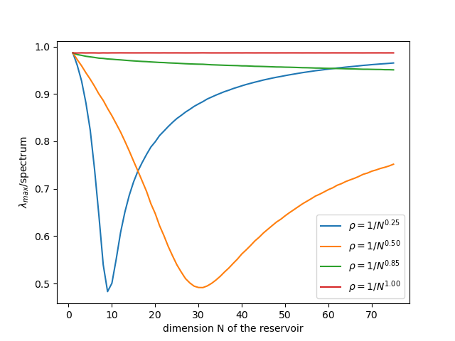
(a) $T=6$

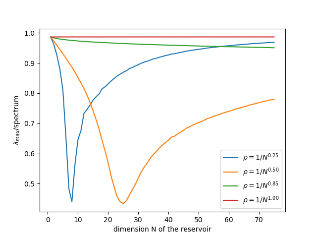
(b) $T=10$

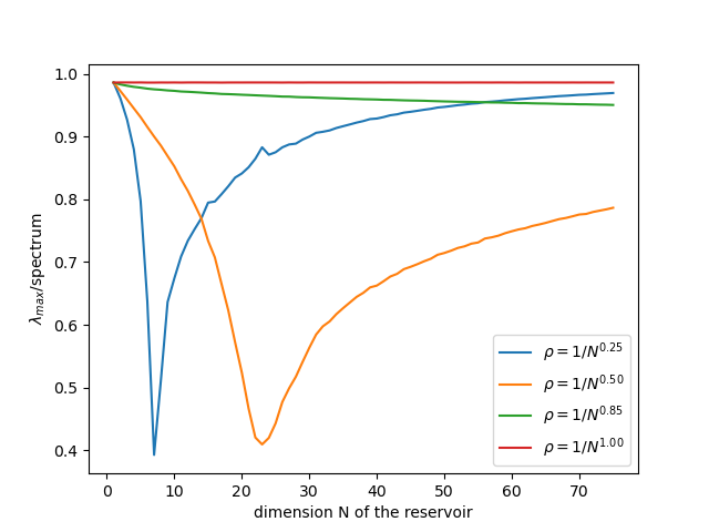
(c) $T=12$

Figure 3. The evolutions in function of the dimension $N$ of the reservoir of the dominance ratio $r_{T,N}$ (as defined in (11)) of the generalised matrix of moments associated to a symmetric $N\times N$ random connectivity matrix with i.i.d. entries on and above the diagonal. These random variables are centred Gaussians with standard deviation $\rho=\frac{1}{N^{\alpha}}$. The different plots correspond to different lengths $T$ of the times-series. The different graphs in each plot correspond to different values of the scaling exponent $\alpha$.

In order to visualise the limiting behaviour of the dominance ratio $r_{T,N}$ at $N$ going to infinity when the symmetric Gaussian connectivity matrix is properly rescaled (i.e. $\alpha=1/2$), we plotted in Figure 4 the evolution of $r_{T}$ (as defined in (4)) in the case of a rescaled Wigner semi-circle distribution (following Theorem 14). In particular, we notice a similar dependence on the value of the factor $\rho$ (appearing in the standard deviation $\frac{\rho}{\sqrt{N}}$) as the one noticed in the 1-dimensional case (Figure 2) and, most importantly, that for a range of values of $T$ (depending on $\rho$), the dominance ratio $r_{T}$ stays well below $1$. Due to the universality of the limiting Wigner semi-circle law, one may reasonably expect this result to generalise for a large class of random symmetric matrices.

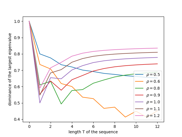
Figure 4. The dominance $r_{T}$ of the largest eigenvalue, in function of the length $T$, over the entire spectrum of the Hankel matrix of moments $A_{\mathrm{sc}}(\rho,\cdot)$ of the rescaled Wigner semi-circle law with rescaling parameter $\rho$.

We turn our attention now to the study of the separation capacity of the reservoir for very long time series. For this purpose, we study the entries of $B_{T,N}$ in function of $T$.

Lemma 17.

Let $N\in\mathbb{N}^{*}$ and $\sigma>0$. Let $W$ be a symmetric $N\times N$ random matrix such that its entries on and above the diagonal are i.i.d. centred Gaussian random variables with standard deviation $\sigma$. For $T\in\mathbb{N}^{*}$, denote by $B_{T,N}$ the generalised matrix of moments of order $T$ of $W$ as given in Definition 7. For $l_{1},l_{2}\in[\![0,T-1]\!]$, one has

$$B_{T,N}(l_{1},l_{2})\leq\frac{1}{\sigma^{2}}\frac{1}{\frac{l_{1}+l_{2}}{\frac{N(N+1)}{2}}+1}B_{T,N}(l_{1}+1,l_{2}+1).$$

Proof.

The inequality is trivial if $l_{1}+l_{2}$ is odd. Assume that $l_{1}+l_{2}$ is even. Let us recall the following identity obtained in the proof of Lemma 12

$$B_{T,N}(l_{1},l_{2})=\sum\limits_{(G,w)\in\mathcal{G}_{N,l_{1}+l_{2}}}E(G,w)N(N-1)\cdots(N-|V_{G}|+1),$$

with $w$ being a loop visiting each edge of $G$ an even number of times. For such a loop $w$, let $k_{w}=2p_{w}$ be the largest amount of times an edge of $G$ is visited by $w$. Note that, trivially

$$\frac{l_{1}+l_{2}}{\frac{N(N+1)}{2}}\leq\frac{l_{1}+l_{2}}{|E_{G}|}\leq k_{w}\leq l_{1}+l_{2}.$$

Let $\tilde{e}(w)$ be the first edge of $G$ that is crossed $k_{w}$ times by $w$. Let $\tilde{w}$ be the walk on $G$ obtained from $w$ by adding a double-crossing of $\tilde{e}(w)$ after it is crossed $k_{w}$ times by $w$. For example, if $w=(1,2,3,3,3,2,1)$, then all edges are visited twice and $k_{w}=2$. Since the self-edge $\{3\}$ is the first edge visited $k_{w}$ times by $w$, then

$$\tilde{w}=(1,2,3,3,3,3,3,2,1).$$

Note that the mapping

$$(G,w)\in\mathcal{G}_{N,l_{1}+l_{2}}\mapsto(G,\tilde{w})\in\mathcal{G}_{N,l_{1}+l_{2}+2}$$

is injective, but not surjective. With the introduced notation, we have the bound

$$E(G,w)=\frac{1}{\sigma^{2}}\frac{m_{k_{w}}}{m_{k_{w}+2}}E(G,\tilde{w})=\frac{1}{\sigma^{2}}\frac{1}{k_{w}+1}E(G,\tilde{w})\leq\frac{1}{\sigma^{2}}\frac{1}{\frac{l_{1}+l_{2}}{\frac{N(N+1)}{2}}+1}E(G,\tilde{w}).$$

Hence, we get

$$\begin{array}[]{rcl}B_{T,N}(l_{1},l_{2})&\leq&\frac{1}{\sigma^{2}}\frac{1}{\frac{l_{1}+l_{2}}{\frac{N(N+1)}{2}}+1}\sum\limits_{(G,w)\in\mathcal{G}_{N,l_{1}+l_{2}}}E(G,\tilde{w})N(N-1)\cdots(N-|V_{G}|+1)\\ &\leq&\frac{1}{\sigma^{2}}\frac{1}{\frac{l_{1}+l_{2}}{\frac{N(N+1)}{2}}+1}\sum\limits_{(G,w)\in\mathcal{G}_{N,l_{1}+l_{2}+2}}E(G,w)N(N-1)\cdots(N-|V_{G}|+1)\\ &=&\frac{1}{\sigma^{2}}\frac{1}{\frac{l_{1}+l_{2}}{\frac{N(N+1)}{2}}+1}B_{T,N}(l_{1}+1,l_{2}+1).\\ \end{array}$$

∎

Similarly to the 1-dimensional case, we show now that the quality of separation deteriorates with time, irrespective of the chosen scaling.

Theorem 18.

Let $N\in\mathbb{N}^{*}$ and $\sigma>0$. Let $W$ be a symmetric $N\times N$ random matrix such that its entries on and above the diagonal are i.i.d. centred Gaussian random variables. For $T\in\mathbb{N}^{*}$, denote by $B_{T,N}$ the generalised matrix of moments of order $T$ of $W$ as given in Definition 7, with eigenvalues denoted

$$\lambda_{T}(B_{T,N})\leq\lambda_{T-1}(B_{T,N})\leq\cdots\leq\lambda_{0}(B_{T,N})(=\lambda_{\mathrm{max}}(B_{T,N})).$$

Then, as $T\to\infty$, $\lambda_{\mathrm{max}}(B_{T,N})$ dominates the spectrum of $B_{T,N}$, i.e.

$$\frac{\lambda_{\mathrm{max}}(B_{T,N})}{\sum\limits_{i=0}^{T}\lambda_{i}(B_{T,N})}\underset{T\to\infty}{\longrightarrow}1.$$

Moreover $\lambda_{\mathrm{max}}(B_{T,N})\underset{T\to+\infty}{\simeq}B_{T,N}(T,T)$.

Proof.

Denote by $\sigma$ the standard variation of the entries of $W$. Following Lemma 17, one has for all $l\in[\![0,T-1]\!]$

$$B_{T,N}(l,l)\leq\frac{1}{\sigma^{2(T-l)}}\prod_{t=l}^{T-1}\frac{1}{\frac{2t}{\frac{N(N+1)}{2}}+1}B_{T,N}(T,T).$$

Therefore

$$1\leq\frac{\mathrm{tr}(B_{T,N})}{B_{T,N}(T,T)}\leq 1+\sum_{l=0}^{T-1}\frac{1}{\sigma^{2(T-l)}}\prod_{t=l}^{T-1}\frac{1}{\frac{2t}{\frac{N(N+1)}{2}}+1}.$$

For any two strictly positive numbers $a$ and $b$, the sequence $(p_{t})_{t\geq 0}$ given by

$$p_{0}=1\quad\text{and}\quad p_{t}=\frac{1\cdot(b+1)\cdot(2b+1)\cdots((t-1)b+1)}{a^{t}}\quad\text{for all }t\geq 1.$$

diverges to $+\infty$. Moreover, it is strictly increasing from a certain rank (that depends on $a$ and $b$.) Hence, there exists $t_{0}\geq 1$ (depending on $a$ and $b$) such that $p_{t}\leq p_{t_{0}}$ for all $1\leq t\leq t_{0}$, and $p_{t}\geq p_{s}$ for all $t\geq s\geq t_{0}$. In particular, one has, for all $T\geq t_{0}+2$

$$\sum_{l=0}^{T-2}p_{l}\leq(T-1)p_{T-2}.$$

Applying this in the case where $a=\frac{1}{\sigma^{2}}$ and $b=\frac{4}{N(N+1)}$, we get that

$$\sum_{l=0}^{T-2}\frac{p_{l}}{p_{T}}=\sum_{l=0}^{T-2}\frac{1}{\sigma^{2(T-l)}}\prod_{t=l}^{T-1}\frac{1}{\frac{2t}{\frac{N(N+1)}{2}}+1}\leq(T-1)\frac{p_{T-2}}{p_{T}}=\frac{1}{\sigma^{4}}\frac{(T-1)}{\left(\frac{4(T-1)}{N(N+1)}+1\right)\left(\frac{4(T-2)}{N(N+1)}+1\right)}.$$

Hence

$$1\leq\frac{\mathrm{tr}(B_{T,N})}{B_{T,N}(T,T)}\leq 1+\frac{1}{\sigma^{2}}\frac{1}{\left(\frac{4(T-1)}{N(N+1)}+1\right)}+\frac{1}{\sigma^{4}}\frac{(T-1)}{\left(\frac{4(T-1)}{N(N+1)}+1\right)\left(\frac{4(T-2)}{N(N+1)}+1\right)}.$$

and $\lim\limits_{T\to\infty}\frac{\mathrm{tr}(B_{T,N})}{B_{T,N}(T,T)}=1$. As a direct consequence of Proposition 8, one has, for all $T\in\mathbb{N}$

$$1\leq\frac{\lambda_{\mathrm{max}}(B_{T,N})}{B_{T,N}(T,T)}\leq\frac{\mathrm{tr}(B_{T,N})}{B_{T,N}(T,T)}.$$

Therefore, one also has $\lim\limits_{T\to\infty}\frac{\lambda_{\mathrm{max}}(B_{T,N})}{B_{T,N}(T,T)}=1$. Thus

$$\frac{\lambda_{\mathrm{max}}(B_{T,N})}{\sum\limits_{t=0}^{T}\lambda_{i}(B_{T,N})}=\frac{\lambda_{\mathrm{max}}(B_{T,N})}{\mathrm{tr}(B_{T,N})}\underset{T\to\infty}{\longrightarrow}1.$$

∎

In Figure 5, we plot the dominance ratio $r_{T,N}$ as a function of $T$ corresponding to different values of the reservoir dimension $N$. We simulated the matrices $B_{T,N}$ using a Monte Carlo method and computed their eigenvalues using the ‘eigenvalsh’ function in Numpy. Due to the instability of the numerical computation of the eigenvalues of very large matrices, we limited ourselves to the maximum value $T=12$.

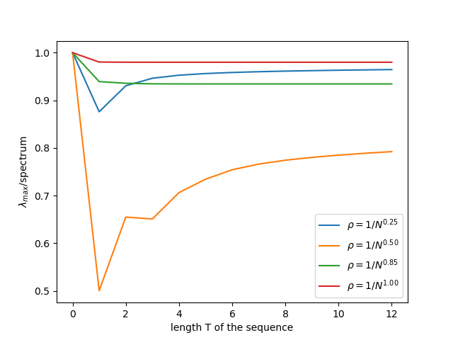
(a) $N=50$

(b) $N=75$

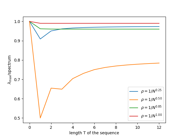
(c) $N=100$

Figure 5. The evolutions in function of the length of the time series $T$ of the dominance ratio $r_{T,N}$ (as defined in (11)) of the generalised matrix of moments associated to a symmetric $N\times N$ random connectivity matrix with i.i.d. entries on and above the diagonal. These random variables are centred and have a standard deviation $\rho=\frac{1}{N^{\alpha}}$. The different plots correspond to different dimensions $N$ of the reservoir. The different graphs in each plot correspond to different values of the scaling exponent $\alpha$.

While Figure 5 may suggest at least a much slower convergence towards $1$ of the dominance ratio $r_{T,N}$ in the case of a scaling $\frac{1}{\sqrt{N}}$, Theorem 18 proves that $r_{T,N}$ converges eventually to $1$. Therefore, we can conclude that the expected separation capacity of reservoirs with symmetric Gaussian connectivity matrices is bound to deteriorate for long time series. When combining this observation with the findings of Theorem 14, we may conclude that random symmetric reservoirs are best suited for relatively short time series, with better quality of separation by large reservoirs ensured when the entries of the reservoir matrix are scaled with the classical factor $\frac{1}{\sqrt{N}}$.

3.2.2. The non-symmetric case

Contrary to the symmetric case, the non-symmetric case is more scarce in the literature of random matrices (at the time of writing, we were only aware of [AD19] leading similar computations). This is due to the fact that the computation of moments (similar to those appearing in inequality (10)) is not equivalent to the convergence of the empirical law of eigenvalues to the circular law ([Bai97, TV08]). However, the computations are fairly similar with the distinction of considering the direction of the walks on the graphs. As before, let us introduce first a couple of notations.

Notation 19.

Let $p,q,N\in\mathbb{N}^{*}$. Given $\mathbf{i}=(i_{1},i_{2},\ldots,i_{p})\in[N]^{p}$ and $\mathbf{j}=(i_{p},j_{2},\ldots,j_{q})\in[N]^{q}$, we denote by $\mathbf{i}\mathbf{j}$ their concatenation given as the $(p+q-1)$-tuple

$$\mathbf{i}\mathbf{j}:=(i_{1},i_{2},\ldots,i_{p},j_{2},\ldots,j_{q}).$$

We denote by $\bar{\mathbf{i}}$ the reverse $p$-tuple

$$\bar{\mathbf{i}}:=(i_{p},i_{p-1},\ldots,i_{1}).$$

Let us now move to our main estimate.

Lemma 20.

Let $N,T\in\mathbb{N}^{*}$, $\rho>0$ and $\alpha\in\mathbb{R}$. Let $W$ be an $N\times N$ random matrix such that its entries are i.i.d. centred Gaussian random variables with standard deviation $\frac{\rho}{N^{\alpha}}$. Denote by $B_{T,N}$ its generalised matrix of moments of order $T$ as given in Definition 7. For $l_{1},l_{2}\in[\![0,T]\!]$, we have the following.

• If $l_{1}+l_{2}$ is odd, then $B_{T,N}(l_{1},l_{2})=0$,

• If $l_{1}+l_{2}$ is even and $\frac{l_{1}+l_{2}}{2}+1\leq N$, then

  $$\begin{array}[]{lcl}\rho^{l_{1}+l_{2}}\frac{N(N-1)\cdots(N-\frac{l_{1}+l_{2}}{2})}{N^{\alpha(l_{1}+l_{2})}}\delta_{l_{1},l_{2}}&\leq&B_{T,N}(l_{1},l_{2})\\ &\leq&\rho^{l_{1}+l_{2}}N^{(l_{1}+l_{2})\left(\frac{1}{2}-\alpha\right)+1}\delta_{l_{1},l_{2}}\\ &&+\rho^{l_{1}+l_{2}}m_{l_{1}+l_{2}}\left(\frac{l_{1}+l_{2}}{2}\right)^{l_{1}+l_{2}}N^{(l_{1}+l_{2})\left(\frac{1}{2}-\alpha\right)},\\ \end{array}$$

  where $\delta_{l_{1},l_{2}}$ is the Kronecker delta symbol.

Proof.

Let $l_{1},l_{2}\in[\![0,T]\!]$. As in the proof of Lemma 12, $B_{T,N}(l_{1},l_{2})$ is trivially null if $l_{1}+l_{2}$ is odd. We assume then that $l_{1}+l_{2}$ is even. Expanding $B_{T,N}(l_{1},l_{2})$, one gets

$$B_{T,N}(l_{1},l_{2})=\mathbb{E}\sum\limits_{\begin{subarray}{c}1\leq i,i_{1},\ldots,i_{l_{1}}\leq N\\ 1\leq j_{1},\ldots,j_{l_{2}}\leq N\end{subarray}}W_{ii_{1}}W_{i_{1}i_{2}}\cdots W_{i_{l_{1}-1}i_{l_{1}}}W_{ij_{1}}W_{j_{1}j_{2}}\cdots W_{j_{l_{2}-1}j_{l_{2}}}.$$

In the above expression, if $j_{l_{2}}\neq i_{l_{1}}$, then the tuple

$$(j_{l_{2}},j_{l_{2}-1},\ldots,j_{1},i,i_{1},i_{2},\ldots,i_{l_{1}})$$

describes a walk on a graph (whose vertices are given by $[N]$) that does not end where it starts. Therefore, one of the edges of this graph is crossed (in some direction) an odd number of times, which implies that the corresponding expectation is null

$$\mathbb{E}W_{ii_{1}}W_{i_{1}i_{2}}\cdots W_{i_{l_{1}-1}i_{l_{1}}}W_{ij_{1}}W_{j_{1}j_{2}}\cdots W_{j_{l_{2}-1}j_{l_{2}}}=0.$$

Consequently

(15) $$\begin{array}[]{rcl}B_{T,N}(l_{1},l_{2})&=&\sum\limits_{\begin{subarray}{c}1\leq i,i_{1},\ldots,i_{l_{1}-1}\leq N\\ 1\leq j,j_{1},\ldots,j_{l_{2}-1}\leq N\end{subarray}}W_{ii_{1}}W_{i_{1}i_{2}}\cdots W_{i_{l_{1}-1}j}W_{ij_{1}}W_{j_{1}j_{2}}\cdots W_{j_{l_{2}-1}j}\\ &=&\sum\limits_{\mathbf{k}=\mathbf{i}\overline{\mathbf{j}}\in\mathcal{I}_{2}(l_{1}+l_{2}+1)}\mathbb{E}W_{\mathbf{i}}W_{\mathbf{j}},\\ \end{array}$$

where, in the above formula,

• we implicitly assume in the decomposition $\mathbf{k}=\mathbf{i}\overline{\mathbf{j}}$ that $\mathbf{i}=(i,i_{1},\ldots,i_{l_{1}-1},j)$ has $l_{1}+1$ elements and that $\mathbf{j}=(i,j_{1},\ldots,j_{l_{2}-1},j)$ has $l_{2}+1$ elements (and both start and end with the same elements.)

• $\mathcal{I}_{2}(l_{1}+l_{2}+1)$ denotes the set of tuples $\mathbf{k}=(k_{1},k_{2},\ldots,k_{l_{1}+l_{2}+1})$ where the first and last elements are equal ($k_{1}=k_{l_{1}+l_{2}+1}$), and where, for all $i\in[l_{1}+l_{1}]$, there exists an even number of elements $p\in[l_{1}+l_{1}]$ such that $\{k_{i},k_{i+1}\}=\{k_{p},k_{p+1}\}$ (otherwise, we will have $\mathbb{E}W_{\mathbf{i}}W_{\mathbf{j}}=0$).

Exactly as in Lemma 12, we map each tuple $\mathbf{k}$ to a pair $(G,w)$, with $G$ being a graph and $w$ a walk on $G$. In such cases let us denote again $\mathbf{k}\sim(G,w)$. Given such a pairing $(G,w)$, where $w$ is of length $L$, we can recover all the $(L+1)$-tuples $\mathbf{k}$ that are mapped to it by injectively mapping the vertices of $G$ to elements in $[N]$. Since we are restricting ourselves in identity (15) to tuples starting and ending at the same points, then the corresponding walk $w$ is necessarily a loop. Let us denote the set of all pairings $(G,w)$ obtained in this manner by $\mathcal{L}_{N,l_{1}+l_{2}}$. As we are restricting ourselves to the set of indices $\mathcal{I}_{2}(l_{1}+l_{2}+1)$ (where each edge is visited an even number of times), then $|E_{G}|\leq\frac{l_{1}+l_{2}}{2}$ and $|V_{G}|\leq\frac{l_{1}+l_{2}}{2}+1$ (by Euler’s formula).

We note again, that given $\mathbf{k}=\mathbf{i}\overline{\mathbf{j}}\in[N]^{l_{1}+l_{2}+1}$, the quantity $\mathbb{E}W_{\mathbf{i}}W_{\mathbf{j}}$ depends only on the pair graph-walk $(G,w)$ associated with $\mathbf{k}$. We denote this quantity $E_{l_{1}}(G,w)$ and remark again that

(16) $$0\leq E_{l_{1}}(G,w)\leq\frac{\rho^{l_{1}+l_{2}}}{N^{\alpha(l_{1}+l_{2})}}m_{l_{1}+l_{2}}.$$

In light of this, identity (15) becomes

$$\begin{array}[]{rcl}B_{T,N}(l_{1},l_{2})&=&\sum\limits_{(G,w)\in\mathcal{L}_{N,l_{1}+l_{2}}}E_{l_{1}}(G,w)\cdot\left|\left\{\mathbf{k}\in\mathcal{I}_{2}(l_{1}+l_{2}+1),\;\;\mathbf{k}\sim(G,w)\right\}\right|\\ &=&\sum\limits_{(G,w)\in\mathcal{L}_{N,l_{1}+l_{2}}}E_{l_{1}}(G,w)N(N-1)\cdots(N-|V_{G}|+1).\\ \end{array}$$

In the above sum, we will separate again two cases.

Case 1: $|V_{G}|=\frac{l_{1}+l_{2}}{2}+1$ (assuming $\frac{l_{1}+l_{2}}{2}+1\leq N$). Then, by Euler’s formula, $|E_{G}|=\frac{l_{1}+l_{2}}{2}$ and $G$ is a tree. Consequently, $w$ crosses each edge of $G$ exactly twice. More exactly, $w$ crosses each edge of $G$ exactly once in each direction (otherwise $G$ will contain a cycle, which will contradict that it is a tree). Let $\mathbf{k}=\mathbf{i}\overline{\mathbf{j}}\sim(G,w)$ be a tuple satisfying this condition and decompose $w=w_{1}\overline{w_{2}}$, where $w_{1}$ corresponds to $\mathbf{i}$ and $w_{2}$ corresponds to $\mathbf{j}$. If an edge is crossed twice (in different directions as per our assumptions) in $w_{i}$, for $i\in\{1,2\}$, then, as this edge cannot be crossed another time in $w$, we get $E_{l_{1}}(G,w)=0$. Hence, we are left with a single configuration, where each edge is crossed once in $w_{1}$ (corresponding to $\mathbf{i}$) then crossed another time in the reverse direction in $\overline{w_{2}}$ or, equivalently, crossed in the same direction in $w_{2}$ (corresponding to $\mathbf{j}$). Obviously, this can only happen if $l_{1}=l_{2}$. In this case, $E_{l_{1}}(G,w)$ is a product of second moments of independent Gaussian random variables. More precisely, we have

$$E_{l_{1}}(G,w)=\frac{\rho^{l_{1}+l_{2}}}{N^{\alpha(l_{1}+l_{2})}}.$$

This implies that

$$\rho^{l_{1}+l_{2}}\frac{N(N-1)\cdots(N-\frac{l_{1}+l_{2}}{2})}{N^{\alpha(l_{1}+l_{2})}}\delta_{l_{1},l_{2}}\leq B_{T,N}(l_{1},l_{2}).$$

Case 2: $|V_{G}|\leq\frac{l_{1}+l_{2}}{2}$. The number of pairings $(G,w)$ satisfying $|V_{G}|\leq\frac{l_{1}+l_{2}}{2}$ is loosely bounded by $\left(\frac{l_{1}+l_{2}}{2}\right)^{l_{1}+l_{2}}$. Using the computation from the previous case when $\frac{l_{1}+l_{2}}{2}+1\leq N$ and the bound (16), we get

$$\begin{array}[]{rcl}B_{T,N}(l_{1},l_{2})&\leq&\rho^{l_{1}+l_{2}}\frac{N(N-1)\cdots(N-\frac{l_{1}+l_{2}}{2})}{N^{\alpha(l_{1}+l_{2})}}\delta_{l_{1},l_{2}}\\ &&+\sum\limits_{\begin{subarray}{c}(G,w)\in\mathcal{L}_{N,l_{1}+l_{2}}\\ |V_{G}|\leq\frac{l_{1}+l_{2}}{2}\end{subarray}}E_{l_{1}}(G,w)N(N-1)\cdots(N-|V_{G}|+1)\\ &\leq&\rho^{l_{1}+l_{2}}N^{(l_{1}+l_{2})\left(\frac{1}{2}-\alpha\right)+1}\delta_{l_{1},l_{2}}+\rho^{l_{1}+l_{2}}m_{l_{1}+l_{2}}\left(\frac{l_{1}+l_{2}}{2}\right)^{l_{1}+l_{2}}N^{(l_{1}+l_{2})\left(\frac{1}{2}-\alpha\right)}.\\ \end{array}$$

∎

Let us now precisely quantify the effect of large dimensions on the separation capacity of a reservoir with a Gaussian connectivity matrix.

Theorem 21.

Let $T\in\mathbb{N}^{*}$, $\rho>0$, $\alpha\in\mathbb{R}$. For $N\in\mathbb{N}^{*}$, let $W_{N}$ be an $N\times N$ random matrix such that its entries are i.i.d. centred Gaussian random variables with standard deviation $\frac{\rho}{N^{\alpha}}$. Let $B_{T,N}$ be its generalised matrix of moments of order $T$ as given in Definition 7, with eigenvalues denoted

$$(\lambda_{\min}(B_{T,N})=)\lambda_{T}(B_{T,N})\leq\lambda_{T-1}(B_{T,N})\leq\cdots\leq\lambda_{0}(B_{T,N})(=\lambda_{\mathrm{max}}(B_{T,N})).$$

• If $\alpha=1/2$, then

  $$\begin{array}[]{ccl}\lambda_{\max}(B_{T,N})&\underset{N\to+\infty}{\simeq}&N\max(1,\rho,\rho^{2},\ldots,\rho^{T}),\\ \lambda_{\min}(B_{T,N})&\underset{N\to+\infty}{\simeq}&N\min(1,\rho,\rho^{2},\ldots,\rho^{T}),\\ \end{array}$$

  and

  $$\lim_{N\to\infty}\frac{\lambda_{\max}(B_{T,N})}{\sum\limits_{i=0}^{T}\lambda_{0}(B_{T,N})}=\frac{\max(1,\rho,\rho^{2},\ldots,\rho^{T})}{\sum\limits_{i=0}^{T}\rho^{i}}.$$

• If $\alpha<1/2$, then

  $$\lambda_{\max}(B_{T,N})\underset{N\to+\infty}{\simeq}\rho^{2T}N^{1+2T\left(\frac{1}{2}-\alpha\right)},$$

  and $\lambda_{\max}(B_{T,N})$ dominates the spectrum of $B_{T,N}$ as $N$ goes to infinity.

• If $\alpha>1/2$, then

  $$\lambda_{\max}(B_{T,N})\underset{N\to+\infty}{\simeq}N,$$

  and $\lambda_{\max}(B_{T,N})$ dominates the spectrum of $B_{T,N}$ as $N$ goes to infinity.

Proof.

For large $N$, Lemma 20 implies

$$\begin{array}[]{ll}\sum\limits_{l=0}^{T}\rho^{2l}\frac{N(N-1)\cdots(N-l)}{N^{2\alpha l}}&\leq\mathbb{E}\sum\limits_{l=0}^{T}B_{T,N}(l,l)\\ &\leq\sum\limits_{l=0}^{T}\left(\rho^{2l}m_{2l}l^{2l}N^{2l\left(\frac{1}{2}-\alpha\right)}+\rho^{2l}N^{1+2l\left(\frac{1}{2}-\alpha\right)}\right).\\ \end{array}$$

Hence

$$\mathrm{tr}(B_{T,N})\underset{N\to+\infty}{\simeq}\sum_{t=0}^{T}\rho^{2t}N^{1+2t\left(\frac{1}{2}-\alpha\right)}.$$

Similarly

$$\|B_{T,N}\|_{2,\infty}\underset{N\to+\infty}{\simeq}\max_{0\leq t\leq T}\rho^{2t}N^{1+2t\left(\frac{1}{2}-\alpha\right)}.$$

Like in the symmetric case, we have the following cases.

Case 1: $\alpha<1/2$. Then (following Proposition 8)

$$\lambda_{\max}(B_{T,N})\underset{N\to+\infty}{\simeq}\rho^{2T}N^{1+2T\left(\frac{1}{2}-\alpha\right)},$$

and $\lambda_{\max}(B_{T,N})$ dominates the spectrum of $B_{T,N}$ as $N$ goes to infinity.

Case 2: $\alpha>1/2$. Then

$$\lambda_{\max}(B_{T,N})\underset{N\to+\infty}{\simeq}N,$$

and $\lambda_{\max}(B_{T,N})$ dominates the spectrum of $B_{T,N}$ as $N$ goes to infinity.

Case 3: $\alpha=1/2$. By Lemma 20, one has

$$\frac{B_{T,N}}{N}\underset{N\to+\infty}{\longrightarrow}\mathrm{diag}(1,\rho,\rho^{2},\ldots,\rho^{T}),$$

where $\mathrm{diag}(1,\rho,\rho^{2},\ldots,\rho^{T})$ is the $(T+1)\times(T+1)$ diagonal matrix whose diagonal is given by $(1,\rho,\rho^{2},\ldots,\rho^{T})$. This yields the claim. ∎

Remark 22.

As noted in the symmetric case, the extra factor $N$ appearing in Theorem 21 is merely due to the norm of the chosen pre-processing vector $u$.

Similarly to the symmetric case, Theorem 21 shows an increase in the largest eigenvalue of $B_{T,N}$ that is at most polynomial in the dimension of the reservoir. We notice again a deterioration in the quality of separation of large reservoirs when the connectivity matrix in not properly rescaled (when $\alpha\neq 1/2$). In Figure 6, we plot the dominance ratio $r_{T,N}$ as a function of $N$ corresponding to different values of $T$. As before, $B_{T,N}$ is simulated using a Monte Carlo method and the eigenvalues computed using Numpy’s ‘eigvalsh’ function.

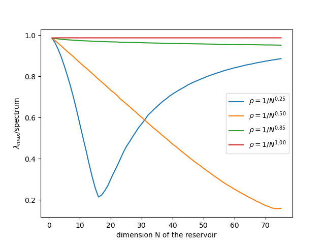
(a) $T=6$

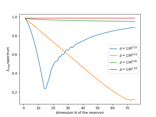
(b) $T=10$

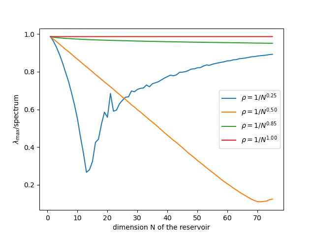
(c) $T=12$

Figure 6. The evolutions in function of the dimension $N$ of the reservoir of the dominance ratio $r_{T,N}$ (as defined in (11)) of the generalised matrix of moments associated to an $N\times N$ random connectivity matrix with i.i.d. Gaussian entries. These random variables are centred and have a standard deviation $\rho=\frac{1}{N^{\alpha}}$. The different plots correspond to different lengths $T$ of the times-series. The different graphs in each plot correspond to different values of the scaling exponent $\alpha$.

Explicit computations can be carried out in this non-symmetric case to show that, for very large and properly rescaled Gaussian reservoirs (i.e. $\alpha=1/2$ and $N\to+\infty$), separation is always most balanced when the factor $\rho$ (appearing in the standard deviation $\frac{\rho}{\sqrt{N}}$) is equal to 1, independently of the value of $T$ (Figure 7), which was not the case in the symmetric case.

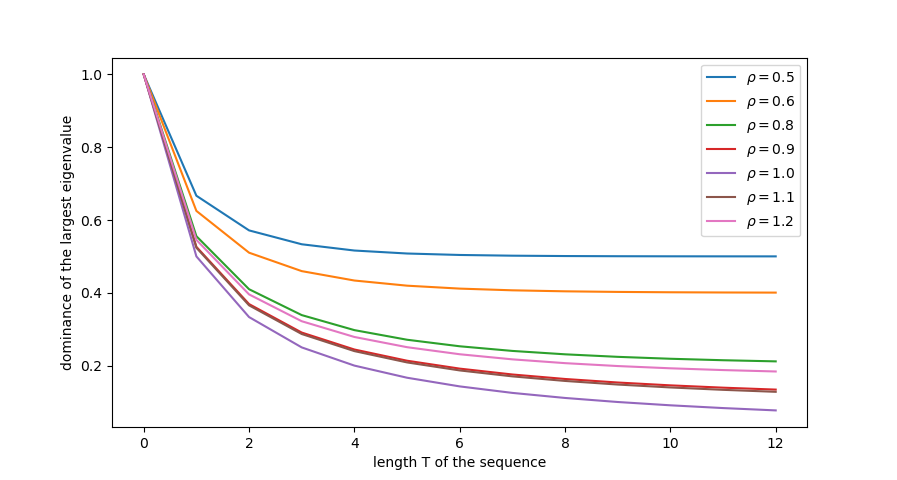
Figure 7. The dominance of the largest eigenvalue, in function of the length $T$, over the entire spectrum of the limit in $N$ of the generalised matrix of moments $B_{T,N}$ associated to a random matrix with i.i.d. centred Gaussian entries with standard deviation $\rho/\sqrt{N}$.

We conclude this section by investigating the evolution of the quality of separation by Gaussian reservoirs (with i.i.d entries) for very long time series. We start with a simple comparative bound of the entries of the matrix of moments $B_{T,N}$.

Lemma 23.

Let $N\in\mathbb{N}^{*}$ and $\sigma>0$. Let $W$ be an $N\times N$ random matrix such that its entries are i.i.d. centred Gaussian random variables with standard deviation $\sigma>0$. For $T\in\mathbb{N}^{*}$, denote by $B_{T,N}$ the generalised matrix of moments of order $T$ of $W$ as given in Definition 7. Then, for all $l_{1},l_{2}\in[\![0,T-1]\!]$

(17) $$B_{T,N}(l_{1},l_{2})\leq\frac{1}{\sigma^{2}N}B_{T,N}(l_{1}+1,l_{2}+1).$$

Additionally, for all $l_{1},l_{2}\in[\![0,T-2]\!]$

(18) $$B_{T,N}(l_{1},l_{2})\leq\frac{1}{\sigma^{4}\left(\frac{l_{1}+l_{2}}{N^{2}}+1\right)}B_{T,N}(l_{1}+2,l_{2}+2).$$

Proof.

The statements are trivial when $l_{1}+l_{2}$ is odd. Assume then that $l_{1}+l_{2}$ is even. Let $\mathbf{i}=(i,i_{1},\ldots,i_{l_{1}-1},j)\in[N]^{l_{1}+1}$ and $\mathbf{j}=(i,j_{1},\ldots,j_{l_{2}-1},j)\in[N]^{l_{2}+1}$ (note that $\mathbf{i}$ and $\mathbf{j}$ start and end with the same elements.) Then, for all $k\in[N]$, one has

$$\sigma^{2}\mathbb{E}W_{\mathbf{i}}W_{\mathbf{j}}\leq\mathbb{E}W_{\mathbf{i}}W_{jk}W_{\mathbf{j}}W_{jk}.$$

This implies

$$\sigma^{2}N\mathbb{E}W_{\mathbf{i}}W_{\mathbf{j}}\leq\sum_{k=1}^{N}\mathbb{E}W_{\mathbf{i}}W_{jk}W_{\mathbf{j}}W_{jk},$$

and therefore (summing over all pairs $(\mathbf{i},\mathbf{j})$)

$$B_{T,N}(l_{1},l_{2})\leq\frac{1}{\sigma^{2}N}B_{T,N}(l_{1}+1,l_{2}+1).$$

Consider now all the $l_{1}+l_{2}$ pairs in the following order

(19) $$(i,i_{1}),(i_{1},i_{2}),\ldots,(i_{l_{1}-1},j),(i,j_{1}),(j_{1},j_{2}),\ldots,(j_{l_{2}-1},j).$$

Let $k_{\mathbf{i},\mathbf{j}}$ be the largest amount of times a pair appears in the above sequence (19), and let $(m,n)$ be the first pair appearing $k_{\mathbf{i},\mathbf{j}}$ times in (19). For obvious reasons, let us only consider the cases where each pair in (19) appears an even number of times. Note that

$$\frac{{l_{1}+l_{2}}}{N^{2}}\leq k_{\mathbf{i},\mathbf{j}}\leq{l_{1}+l_{2}}.$$

We have then

$$\sigma^{4}\left(\frac{l_{1}+l_{2}}{N^{2}}+1\right)\mathbb{E}W_{\mathbf{i}}W_{\mathbf{j}}\leq\sigma^{4}(k_{\mathbf{i},\mathbf{j}}+1)\mathbb{E}W_{\mathbf{i}}W_{\mathbf{j}}=\sigma^{4}\frac{m_{k_{\mathbf{i},\mathbf{j}}+2}}{m_{k_{\mathbf{i},\mathbf{j}}}}\mathbb{E}W_{\mathbf{i}}W_{\mathbf{j}}\leq\mathbb{E}W_{\mathbf{i}}W_{jm}W_{mn}W_{\mathbf{j}}W_{jm}W_{mn}.$$

Therefore

$$B_{T,N}(l_{1},l_{2})\leq\frac{1}{\sigma^{4}\left(\frac{l_{1}+l_{2}}{N^{2}}+1\right)}B_{T,N}(l_{1}+2,l_{2}+2).$$

∎

As a consequence of the above bounds, we have the following lower bounds on the dominance ratio $r_{T,N}$ in function of the length $T$ of the time series.

Theorem 24.

Let $N\in\mathbb{N}^{*}$ and $\sigma>0$. Let $W$ be an $N\times N$ random matrix such that its entries are i.i.d. centred Gaussian random variables with standard deviation $\sigma>0$. For $T\in\mathbb{N}^{*}$, denote by $B_{T,N}$ the generalised matrix of moments of order $T$ of $W$ as given in Definition 7, with eigenvalues denoted

$$\lambda_{T}(B_{T,N})\leq\lambda_{T-1}(B_{T,N})\leq\cdots\leq\lambda_{0}(B_{T,N})(=\lambda_{\mathrm{max}}(B_{T,N})).$$

Then, for all $T\in\mathbb{N}$

$$\frac{1}{P(T)}\leq\frac{\lambda_{\max}(B_{T,N})}{\sum\limits_{i=0}^{T}\lambda_{i}(B_{T,N})}\leq 1,$$

where

$$P(T)=\min\left(T+1,\sum_{l=0}^{T}(\sigma^{2}N)^{-l}\right).$$

Moreover, there exists $T_{\sigma,N}>0$, such that, for all $T\geq T_{\sigma,N}$, one has

$$\frac{1}{Q(T)}\leq\frac{\lambda_{\max}(B_{T,N})}{\sum\limits_{i=0}^{T}\lambda_{i}(B_{T,N})},$$

where

$$Q(T):=\min\left(2,1+\frac{1}{\sigma^{2}N}\right)\left(1+\frac{1}{2\left(\frac{\sigma^{2}}{N}\right)^{2}(T-3)}+\frac{T}{8\left(\frac{\sigma^{2}}{N}\right)^{4}(T-5)^{2}}\right).$$

Proof.

A recursive argument using the bound (17) in Lemma 23, gives

$$\mathrm{tr}(B_{T,N})\leq\sum_{l=0}^{T}\frac{1}{(\sigma^{2}N)^{l}}B_{T,N}(T,T).$$

Thus

$$\left(\sum_{l=0}^{T}\frac{1}{(\sigma^{2}N)^{l}}\right)^{-1}\leq\frac{B_{T,N}(T,T)}{\mathrm{tr}(B_{T,N})}\leq\frac{\lambda_{\max}(B_{T,N})}{\mathrm{tr}(B_{T,N})},$$

which yields the first bound. Let $l\in[\![0,T]\!]$. If $T-l$ is even and $T-l\geq 2$, the bound (18) gives

$$B_{T,N}(l,l)\leq\prod_{t=0}^{\frac{T-l}{2}-1}\frac{1}{\sigma^{4}\left(\frac{2(l+2t)}{N^{2}}+1\right)}B_{T,N}(T,T)=\prod_{k=1}^{\frac{T-l}{2}}\frac{1}{\sigma^{4}\left(\frac{2(T-2k)}{N^{2}}+1\right)}B_{T,N}(T,T).$$

If $T-l$ is odd and $T-l\geq 3$, we similarly have

$$B_{T,N}(l,l)\leq\prod_{k=1}^{\frac{T-l-1}{2}}\frac{1}{\sigma^{4}\left(\frac{2(T-1-2k)}{N^{2}}+1\right)}B_{T,N}(T-1,T-1).$$

We have then

$$\sum_{T-l\text{ even}}B_{T,N}(l,l)\leq\left(1+\sum_{p=1}^{\lfloor T/2\rfloor}\prod_{k=1}^{p}\frac{1}{\sigma^{4}\left(\frac{2(T-2k)}{N^{2}}+1\right)}\right)B_{T,N}(T,T).$$

Employing a similar technique than in the proof of Theorem 18, we can show that for $T$ larger than $T^{(1)}_{\sigma,N}$ (depending only on $\sigma$ and $N$), one has

$$\sum_{T-l\text{ even}}B_{T,N}(l,l)\leq\left(1+\frac{1}{\sigma^{4}\left(\frac{2(T-2)}{N^{2}}+1\right)}+\frac{1}{\sigma^{8}}\frac{\lfloor T/2\rfloor-1}{\left(\frac{2(T-2)}{N^{2}}+1\right)(\frac{2(T-4)}{N^{2}}+1)}\right)B_{T,N}(T,T).$$

Similarly, for $T$ larger than $T^{(2)}_{\sigma,N}$ (depending only on $\sigma$ and $N$), one also has

$$\sum_{T-l\text{ odd}}B_{T,N}(l,l)\leq\left(1+\frac{1}{\sigma^{4}\left(\frac{2(T-3)}{N^{2}}+1\right)}+\frac{1}{\sigma^{8}}\frac{\lfloor\frac{T-1}{2}\rfloor-1}{\left(\frac{2(T-3)}{N^{2}}+1\right)(\frac{2(T-5)}{N^{2}}+1)}\right)B_{T,N}(T-1,T-1).$$

Note that (using again the bound (17))

$$B_{T,N}(T,T)+B_{T,N}(T-1,T-1)\leq\min\left(2,1+\frac{1}{\sigma^{2}N}\right)\lambda_{\max}(B_{T,N}).$$

Hence, defining

$$Q_{0}(T):=1+\frac{1}{2\left(\frac{\sigma^{2}}{N}\right)^{2}(T-3)}+\frac{T}{8\left(\frac{\sigma^{2}}{N}\right)^{4}(T-5)^{2}},$$

we get, for $T\geq T_{\sigma,N}:=\max\left(T^{(1)}_{\sigma,N},T^{(2)}_{\sigma,N}\right)$

$$\mathrm{tr}(B_{T,N})\leq Q_{0}(T)(B_{T,N}(T,T)+B_{T,N}(T-1,T-1))\leq Q(T)\lambda_{\max}(B_{T,N}).$$

This yields the result. ∎

Contrary to the symmetric case, Thereom 24 does not show a definitive deterioration in the quality of separation (understood as $(r_{T,N})_{T\geq 1}$ converging to $1$ as $T$ goes to infinity) of very long time series by reservoirs whose Gaussian connectivity matrices have i.i.d. entries (although a convergence of $(r_{T,N})_{T\geq 1}$ towards $1$ might still hold). However, the combination of the two bounds in Thereom 24 does point to a deterioration in the quality of separation by reservoirs whose matrices are very badly scaled, i.e. when $\sigma$ is very far from $1/\sqrt{N}$ (although these bounds might not always be sharp.) In Figure 5, we plot the dominance ratio $r_{T,N}$ as a function of $T$ corresponding to different values of the reservoir dimension $N$. As in the inequalities from Thereom 24, the plots point to a superiority of reservoir matrices having a standard variation close to $1/\sqrt{N}$, with the quality of separation improving with larger values of $N$.

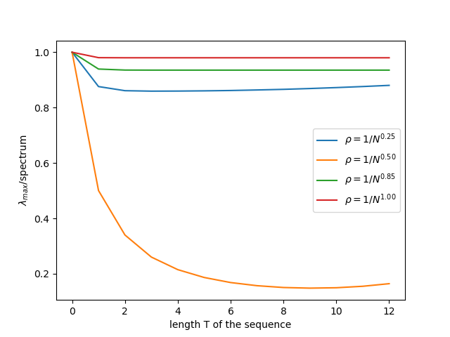
(a) $N=50$

(b) $N=75$

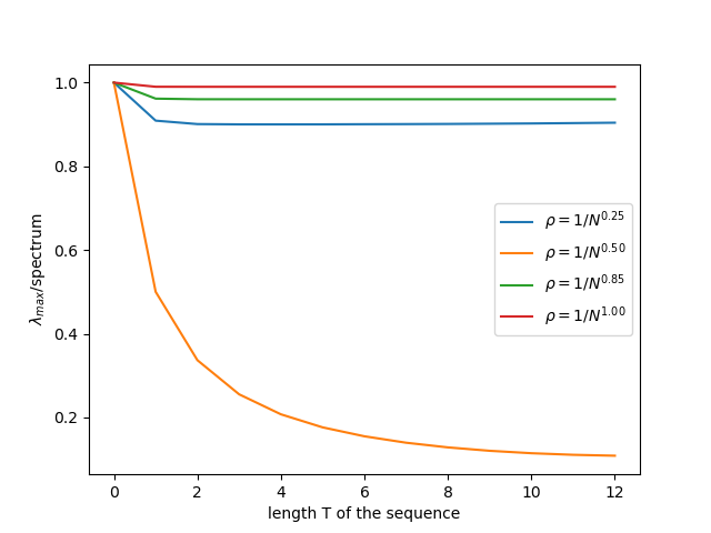
(c) $N=100$

Figure 8. The evolutions in function of the length of the time series $T$ of the dominance ratio $r_{T,N}$ (as defined in (11)) of the generalised matrix of moments associated to an $N\times N$ random connectivity matrix with i.i.d. Gaussian entries. These random variables are centred and have a standard deviation $\rho=\frac{1}{N^{\alpha}}$. The different plots correspond to different dimensions $N$ of the reservoir. The different graphs in each plot correspond to different values of the scaling exponent $\alpha$.

Remark 25.

More care is needed when taking both $T$ and $N$ going to infinity; in the sense that one needs to know as which rate both quantities grow. Indeed, considering the case of the scaling $\sigma=1/\sqrt{N}$, Thereom 21 shows that, for all $T\geq 0$, one has

$$\lim_{N\to+\infty}r_{T,N}=\frac{1}{T+1},$$

Hence

$$\lim_{T\to+\infty}\left(\lim_{N\to+\infty}r_{T,N}\right)=0.$$

However, the second bound from Thereom 24 shows that, for every $N\in\mathbb{N}^{*}$ and $\varepsilon>0$, for large values of $T$, one has $\frac{1}{2}-\varepsilon\leq r_{T,N}$. This observation hints that an optimal implementation in practice is achieved when taking $N\gg T$ (and a scaling of the entries $\sigma=1/\sqrt{N}$.)

4. Probabilistic separation guarantees

In light of the results of Section 3, it is natural to ask whether an expected separation translates into a high probability of separation. In this section, we will aim to answer this question by giving quantitative probabilistic bounds on the separation capacity of random reservoirs.

4.1. A probabilistic bound for the 1-dimensional random reservoir

We will first expose a technique that highlights the explicit dependence of the likelihood of separation on the temporal geometry of the time series in the one-dimensional case. Let us recall the following classical bound on the modulus of the largest root of a complex polynomial (which is attributed to Zassenhaus but can be traced back to Lagrange).

Lemma 26 ([Yap00]).

Let $T\in\mathbb{N}^{*}$. Let

$$f(w)=\sum_{t=0}^{T}a_{T-t}w^{t}$$

be a (complex) polynomial of degree $T$, i.e. $a_{0}\neq 0$. Define the following quantity

(20) $$\beta(f):=2\max\left(\left|\frac{a_{1}}{a_{0}}\right|,\left|\frac{a_{2}}{a_{0}}\right|^{1/2},\ldots,\left|\frac{a_{T}}{a_{0}}\right|^{1/T}\right).$$

If $w_{0}\in\mathbb{C}$ is a root of $f$, then $|w_{0}|<\beta(f)$.

Using the above bound on the roots of a polynomial, we get the following probabilistic bound on the separation of the outputs of two different times series by a random linear reservoir.

Lemma 27.

Let $\varepsilon>0$ and $T\in\mathbb{N}^{*}$. Let $w$ be a real-valued random variable and $\mathbf{a}:=(a_{t})_{0\leq t\leq T}$ be sequence of real numbers such that $a_{0}\neq 0$. Let $K>0$ be such that $\mathbf{a}$ exhibits the following geometric evolution

$$\forall t\in[\![0,T-1]\!]\colon|a_{t}|\leq K^{t}|a_{0}|,\quad|a_{T}+\varepsilon|\leq K^{T}|a_{0}|\quad\text{and}\quad|a_{T}-\varepsilon|\leq K^{T}|a_{0}|.$$

Then

$$\mathbb{P}(|f(\mathbf{a},w)|\geq\varepsilon)\geq\mathbb{P}(|w|\geq 2K),$$

where $f(\mathbf{a},w)$ denotes the output of the $1$-dimensional random reservoir with connectivity $w$ and time series $\mathbf{a}$, i.e.

$$f(\mathbf{a},w)=\sum_{t=0}^{T}a_{T-t}w^{t}.$$

Proof.

The time series $\mathbf{a}$ being fixed, we will drop referring to it in $f$. Let us note that the geometric evolution assumptions imply

(21) $$\max(\beta(f-\varepsilon),\beta(f+\varepsilon))\leq 2K,$$

where $\beta$ refers to the Zassenhaus-Lagrange bound (20). Without loss of generality, we will assume that $a_{0}>0$. Let $x\in\mathbb{R}$.

• Assume $x\geq 2K$. Then (by the bound (21) and Lemma 26) $f-\varepsilon$ has no roots on $[2K,+\infty)$. Hence it is positive on this interval. Therefore $f(x)=|f(x)|\geq\varepsilon$.

• Assume $x\leq-2K$. If $T$ is even, then $f-\varepsilon$ has no roots on $(-\infty,-2K]$ and is positive on this interval. Therefore $f(x)=|f(x)|\geq\varepsilon$. If $T$ is odd, $f+\varepsilon$ is negative on $(-\infty,-2K]$. Hence $f(x)=-|f(x)|\leq-\varepsilon$.

The above analysis shows that

$$\left\{|w|\geq 2K\right\}\subseteq\left\{|f(\mathbf{a},w)|\geq\varepsilon\right\},$$

which trivially leads to the sought inequality. ∎

Remark 28.

With $T$ and $\mathbf{a}$ being fixed, there always exists a positive number $K$ such that the geometric decay hypothesis in the above lemma holds.

Building on the above, the following corollary shows that a larger hyperparameter allows for a better likelihood of large separation.

Corollary 29.

Let $\varepsilon>0$, $\rho>0$ and $T\in\mathbb{N}^{*}$. Let $w$ be a real-valued random variable and $\mathbf{a}:=(a_{t})_{0\leq t\leq T}$ be a sequence of real numbers such that $a_{0}\neq 0$. Let $K>0$ be such that $\mathbf{a}$ exhibits the following geometric evolution

(22) $$\forall t\in[\![0,T-1]\!]\colon|a_{t}|\leq(K\rho)^{t}|a_{0}|,\quad|a_{T}+\varepsilon|\leq(K\rho)^{T}|a_{0}|\quad\text{and}\quad|a_{T}-\varepsilon|\leq(K\rho)^{T}|a_{0}|.$$

Then

$$\mathbb{P}(|f(\mathbf{a},\rho w)|\geq\varepsilon)\geq\mathbb{P}(|w|\geq 2K),$$

where $f(\mathbf{a},\rho w)$ denotes the output of the $1$-dimensional random reservoir with connectivity $\rho w$ and time series $\mathbf{a}$.

Proof.

This is a straightforward application of Lemma 27. ∎

The above corollary highlights an important role of the hyperparameter $\rho$. One may freely choose $K$ to be small as to make $\mathbb{P}(|w|\geq 2K)$ large, then choose $\rho$ large enough so that the geometric evolution hypothesis (22) holds; the only constraint being the numerical stability of the computations.

Let us now apply this result to a couple of classical examples.

Example 3.

Let $w$ be a Rademacher random variable. Let $\rho>0$ such that

(23) $$\rho\geq 2\max\left(\left|\frac{a_{1}}{a_{0}}\right|,\left|\frac{a_{2}}{a_{0}}\right|^{1/2},\cdots,\left|\frac{a_{T-1}}{a_{0}}\right|^{1/(T-1)},\left|\frac{a_{T}+\varepsilon}{a_{0}}\right|^{1/T},\left|\frac{a_{T}-\varepsilon}{a_{0}}\right|^{1/T}\right).$$

Then $\mathbb{P}(|f(\mathbf{a},\rho w)|\geq\varepsilon)=1$. Indeed, this is a direct application of Corollary 29 with $K=1/2$. Consequently, we can deterministically ensure the separation of two signals with a Rademacher random reservoir with large enough hyperparameter $\rho$. Note that this is not in contradiction with the results of Subsection 3.1 (Example 1) where we found that the dimension of the space

$$D_{w}:=\left\{\mathbf{a}\colon\;f(\mathbf{a},w)=0\;\;\text{almost surely}\right\}$$

is $T-2$. Indeed, inequality (23) merely ensures that $\mathbf{a}\notin D_{\rho w}$ (the latter space still being of dimension $T-2$). Conversely, if $\mathbf{a}\in D_{w}$, one can ensure separability by modulating the random variable $w$ by a hyperparameter $\rho$ satisfying inequality (23). Hence, in this case, one can ensure separation by choosing a large hyperparameter $\rho$ (at the expense of stability and a computational cost) and without a spectral analysis of the corresponding Hankel matrix of moments. This being said, the order of magnitude of such $\rho$ directly depends on the considered data.

Example 4.

Let $w$ be a standard Gaussian random variable. Let $\delta\in(0,1)$. Denote by $\Phi$ the Gaussian cumulative distribution function. Let (omitting the dependence on $\mathbf{a}$)

$$\rho_{\delta,\varepsilon}=\frac{2}{\Phi^{-1}\left(\frac{1+\delta}{2}\right)}\max\left(\left|\frac{a_{1}}{a_{0}}\right|,\left|\frac{a_{2}}{a_{0}}\right|^{1/2},\cdots,\left|\frac{a_{T-1}}{a_{0}}\right|^{1/(T-1)},\left|\frac{a_{T}+\varepsilon}{a_{0}}\right|^{1/T},\left|\frac{a_{T}-\varepsilon}{a_{0}}\right|^{1/T}\right).$$

Then $\mathbb{P}(|f(\mathbf{a},\rho_{\delta,\varepsilon}w)|\geq\varepsilon)\geq 1-\delta$. Indeed, this is an application of Corollary 29 with

$$K_{\delta}=\frac{1}{2}\Phi^{-1}\left(\frac{1+\delta}{2}\right).$$

Using this technique, we see that if we require a probability of separation at least

$$1-\delta^{*}=2(1-\Phi(1))\approx 0.317,$$

then we require a hyperparameter $\rho_{\delta,\varepsilon}$ that is larger than or equal to the one required in the Rademacher case (inequality (23)). However, one can cast away this concern as a limit of the technique we used (which ignores what happens exactly in the interval $[-\beta(f),\beta(f)]$ where roots of $f$ may lie) and the fact that the Gaussian distribution ensures separation in expectation for all time series since the kernel of the quadratic form associated to it is non-singular (as seen in Subsection 3.1.)

4.2. Probabilistic guarantees via concentration inequalities

The technique detailed in the previous subsection does not generalise easily to the higher dimensional case (where finite sets of roots are to be replaced by affine algebraic sets). As the expectation of separation is positive in the cases we are interested in (such as connectivity matrices with Gaussian entries), a reasonable approach is to quantify the probability of separation through the concentration of the distance between two outputs around its mean (which was studied in the first section.) However, one cannot reasonably expect the concentration to hold with very high probability, as polynomials do not have good concentration properties in general. We suspect that this could be a reason why introducing suitable non-linear activation functions lead to better results. In this subsection, we will give generic probabilistic guarantees using concentration inequalities. Before we delve into these, some definitions, notations and conventions are needed.

Definition 30.

Let $S$ be a non-empty set and $k\in\mathbb{N}^{*}$. For each $i\in[k]$, let $J_{i}$ be a non-empty subset of $S$. We say that the collection $\mathcal{J}=\{J_{1},J_{2},\ldots,J_{k}\}$ is a partition of $S$, and denote $\mathcal{J}\in\mathcal{P}(S)$, if the following two conditions are satisfied:

• $\cup_{i=1}^{k}J_{i}=S$,

• $J_{i}\cap J_{j}=\emptyset$ for all $i,j\in[k]$ such that $i\neq j$.

The following indexation notation will be very convenient.

Notation 31.

Let $n,d,k,p\in\mathbb{N}^{*}$. Let $J=\{j_{1}<j_{2}<\cdots<j_{p}\}$ be a non-empty subset of $[d]$. Let $\mathbf{i}=(i_{1},\ldots,i_{d})\in[n]^{d}$ and $x$ be a $p$-tensor in $\mathbb{R}^{n}$ (i.e. $x\in(\mathbb{R}^{n})^{\otimes p}$). We denote by $x_{\mathbf{i}_{J}}$ the element

$$x_{\mathbf{i}_{J}}:=x_{i_{j_{1}}i_{j_{2}}\ldots i_{j_{p}}}.$$

More formally, if we think of $x$ as a map from $[n]^{p}$ to $\mathbb{R}$ ($x(i_{1},\ldots,i_{p})=x_{i_{1}\ldots i_{p}}$), of $\mathbf{i}$ as a map from $[d]$ to $[n]$ ($\mathbf{i}(r)=i_{r}$), and of $J$ as the $p$-tuple $(j_{1},j_{2},\ldots,j_{p})$, then

$$x_{\mathbf{i}_{J}}=x(\mathbf{i}(J)).$$

For instance, if $d=4$ and $J=\{1,3\}$ then $x_{\mathbf{i}_{J}}=x_{i_{1}i_{3}}$. We introduce now the Hilbert–Schmidt norm of a tensor.

Notation 32.

Let $n,p\in\mathbb{N}^{*}$ and $x$ be a $p$-tensor in $\mathbb{R}^{n}$ (i.e. $x\in(\mathbb{R}^{n})^{\otimes p}$). We denote by $\|x\|_{\mathrm{HS}}$ the Hilbert–Schmidt norm of $x$ given by

$$\|x\|_{\mathrm{HS}}:=\left(\sum_{1\leq i_{1},\ldots,i_{p}\leq n}x_{i_{1}i_{2}\ldots i_{p}}^{2}\right)^{1/2}.$$

We introduce furthermore the following family of tensor norms.

Definition 33.

Let $n,d,k\in\mathbb{N}^{*}$. Let $A=(a_{i_{1}i_{2}\cdots i_{d}})_{1\leq i_{1},i_{2},\ldots,i_{d}\leq n}$ be a $d$-tensor in $\mathbb{R}^{n}$ (i.e. $A\in(\mathbb{R}^{n})^{\otimes d}$). Let $\mathcal{J}=\{J_{1},J_{2},\ldots,J_{k}\}\in\mathcal{P}([d])$. We denote by $\|A\|_{\mathcal{J}}$ the following norm

$$\begin{array}[]{l}\|A\|_{\mathcal{J}}:=\\ \sup\left\{\sum\limits_{\mathbf{i}=(i_{1},i_{2},\ldots,i_{d})\in[n]^{d}}a_{i_{1}i_{2}\cdots i_{d}}x^{(1)}_{\mathbf{i}_{J_{1}}}\cdots x^{(k)}_{\mathbf{i}_{J_{k}}};\;\;x^{(p)}\in(\mathbb{R}^{n})^{\otimes|J_{p}|}\text{ and }\|x^{(p)}\|_{\mathrm{HS}}\leq 1\textrm{ for all }p\in[k]\right\}.\end{array}$$

Let us illustrate the above by a couple of examples (see also [AW15, Lat06].)

Examples 1.

1. First, let us take the case $d=2$. For a matrix $A\in\mathbb{R}^{n\times n}$, we have the following.

   $$\begin{array}[]{c}\|A\|_{\{1,2\}}=\sup\left\{\sum\limits_{1\leq i,j\leq n}a_{ij}x_{ij};\;\;x\in\mathbb{R}^{n\times n}\text{ and }\|x\|_{\mathrm{HS}}\leq 1\right\}=\|A\|_{\mathrm{HS}},\\ \|A\|_{\{\{1\},\{2\}\}}=\sup\left\{\sum\limits_{1\leq i,j\leq n}a_{ij}x_{i}y_{j};\;\;x,y\in\mathbb{S}^{n-1}\right\}=\|A\|_{\mathrm{op}}.\end{array}$$

2. In the case $d=3$, taking $\mathcal{J}=\{\{1,3\},\{2\}\}$ gives, for $A\in(\mathbb{R}^{n})^{\otimes 3}$

   $$\|A\|_{\{\{1,3\},\{2\}\}}=\sup\left\{\sum_{1\leq i,j,k\leq n}a_{ijk}x_{ik}y_{j};\;\;x\in(\mathbb{R}^{n})^{\otimes 2}\text{ and }\sum_{1\leq i,k\leq n}x_{ik}^{2}\leq 1,y\in\mathbb{S}^{n-1}\right\}.$$

Finally, let us recall the identification between successive Fréchet derivatives and tensors. Given a smooth function $f\colon\mathbb{R}^{n}\to\mathbb{R}$ and $k\in\mathbb{N}$, then its $k$^th Fréchet derivative $f^{(k)}$ is a map defined on $\mathbb{R}^{n}$ with values in $\mathcal{L}_{s}((\mathbb{R}^{n})^{\otimes k},\mathbb{R})$, the space of symmetric $k$-linear mappings from a $\mathbb{R}^{n}$ to $\mathbb{R}$. Hence, given $x\in\mathbb{R}^{n}$, $f^{(k)}(x)$ can be canonically represented as an element $A$ of $(\mathbb{R}^{n})^{\otimes k}$ using the canonical basis of $\mathbb{R}^{n}$

$$A=(f^{(k)}(x)(e_{i_{1}}\otimes e_{i_{2}}\otimes\cdots\otimes e_{i_{k}}))_{1\leq i_{1},i_{2},\ldots,i_{k}\leq n}=\left(\frac{\partial^{k}f}{\partial x_{i_{1}}\partial x_{i_{2}}\cdots\partial x_{i_{k}}}(x)\right)_{1\leq i_{1},i_{2},\ldots,i_{k}\leq n},$$

where $(e_{1},\ldots,e_{n})$ is the canonical basis of $\mathbb{R}^{n}$. We are now ready to state the key concentration inequality.

Theorem 34 ([AW15]).

Let $n,D\in\mathbb{N}^{*}$. Let $G$ be a standard $n$-dimensional Gaussian random vector. Let $P$ be a multivariate polynomial of $n$ variables that is of degree $D$. There exists a constant $C_{D}>0$, such that, for all $t>0$,

$$\frac{1}{C_{D}}\exp\left(-C_{D}\eta(t)\right)\leq\mathbb{P}\left(|P(G)-\mathbb{E}P(G)|\geq t\right)\leq C_{D}\exp\left(-\frac{1}{C_{D}}\eta(t)\right),$$

where

$$\eta(t)=\min_{1\leq k\leq D}\min_{\mathcal{J}\in P([k])}\left(\frac{t}{\|\mathbb{E}P^{(k)}(G)\|_{\mathcal{J}}}\right)^{2/|\mathcal{J}|}.$$

Let us note that the upper bound in Theorem 34 generalises to wider classes of random vectors, for example those with entries satisfying a logarithmic Sobolev inequality ([AW15]) or those with sub-Gaussian or sub-exponential entries ([GSS21]). The same applies for a wider class of functions than polynomials, for example functions $f$ with uniformly bounded $D$^th derivative. However, for simplicity and a more complete analysis, we will restrict ourselves to the bound above.

In the following, let us consider an $N$-dimensional (linear) random reservoir acting on a time series $\mathbf{a}=(a_{t})_{0\leq t\leq T}$ modelling the difference of two time series $\mathbf{x}$ and $\mathbf{y}$. As before, we are interested in the random distance

$$\|f(\mathbf{a},W)\|_{2}=\|f(\mathbf{x},W)-f(\mathbf{y},W)\|_{2}.$$

The idea now is to use the concentration inequality in Theorem 34 to quantify the probability of the separation of the outputs of the two time series by the random reservoir, while leveraging the knowledge that the expected separation is strictly positive (when the entries of the connectivity matrix are Gaussian for example.) In our case, the squared distance $\|f(\mathbf{a},W)\|^{2}_{2}$, which is a polynomial of degree $2T$, will play the role of the multivariate polynomial $P$ in Theorem 34. In practice, while there exists good algorithms for the computation of partial derivatives of multivariate polynomials (e.g. [CG90]), the exact computation of the quantities $\|\mathbb{E}P^{(k)}(G)\|_{\mathcal{J}}$ is out of question due to the complexity of the norms in Definition 33 and the need for a large number of samples to approximate the expectations. Moreover, Theorem 34 gives general conservative bounds that may be far from sharp in particular situations. Consequently, Theorem 34 will mostly serve as a guideline as to how the probability of separation is influenced by the different parameters of the practical implementation of the reservoir.

The first obvious remark is that the squared distance $\|f(\mathbf{a},W)\|^{2}_{2}$ does not fully concentrate around its expectation: the probability

$$\mathbb{P}\left(|\|f(\mathbf{a},W)\|^{2}_{2}-\mathbb{E}\|f(\mathbf{a},W)\|^{2}_{2}|\geq t\right)$$

is always strictly positive. Minimising this probability requires taking a large value for $t$, which is only sensible as long as $t<\mathbb{E}\|f(\mathbf{a},W)\|^{2}_{2}$ (otherwise, the event

$$\{|\|f(\mathbf{a},W)\|^{2}_{2}-\mathbb{E}\|f(\mathbf{a},W)\|^{2}_{2}|\geq t\}$$

will exclude small near-zero values for $\|f(\mathbf{a},W)\|^{2}_{2}$).

The second remark is that when it is sensible to take large values for $t$ in Theorem 34, the probability

$$\mathbb{P}\left(|\|f(\mathbf{a},W)\|^{2}_{2}-\mathbb{E}\|f(\mathbf{a},W)\|^{2}_{2}|\geq t\right)$$

decays like

$$\exp\left(-\frac{t^{1/T}}{C_{2T}M_{a_{0},T,W}}\right),$$

where $M_{a_{0},T,W}$ depends only on $a_{0}$, $T$ and the chosen distribution for the connectivity matrix $W$. Hence the concentration phenomena worsens with longer time series. Perhaps one can expect these observed non-concentration properties to improve under the application of appropriate non-linear activation functions such as $\tanh$.

The third remark is that, while we simply compared the expected square distance of outputs $\mathbb{E}\|f(\mathbf{a},W)\|^{2}_{2}$ to the square distance between time series $\|\mathbf{a}\|^{2}_{2}$ in the previous section, the concentration of the square distance $\|f(\mathbf{a},W)\|^{2}_{2}$ around its mean is not simply characterised by the distance $\|\mathbf{a}\|^{2}_{2}$. Theorem 34 highlights, through the successive derivatives of the polynomial, the role of the order in which the input information occurs. Let us explicit this dependence in the one-dimensional case. The following is a direct trivial consequence of Theorem 34.

Corollary 35.

Let $w$ be a standard Gaussian real random variable. Let $T\in\mathbb{N}^{*}$. There exists a constant $C_{T}>0$ depending only on $T$ such that, for all $\mathbf{a}\in\mathbb{R}^{T+1}$ and $t>0$, one has

$$\frac{1}{C_{T}}\exp\left(-C_{T}\eta(t)\right)\leq\mathbb{P}\left(|f^{2}(\mathbf{a},w)-\mathbb{E}f^{2}(\mathbf{a},w)|\geq t\right)\leq C_{T}\exp\left(-\frac{1}{C_{T}}\eta(t)\right),$$

where

$$\eta(t)=\min_{1\leq p\leq k\leq 2T}\left(\frac{t}{|\mathbb{E}\frac{\partial(f^{2})^{(k)}}{\partial w^{k}}(\mathbf{a},w)|}\right)^{2/p}.$$

Consider now the following simple example.

Example 5.

Consider the simple case of $T=2$ and $w\sim\mathcal{N}(0,1)$. For $\mathbf{x}=(x_{0},x_{1},x_{2})$, one easily gets

$$\begin{array}[]{cc}\mathbb{E}f^{2}(\mathbf{x},w)=3x_{0}^{2}+x_{1}^{2}+2x_{0}x_{2}+x_{2}^{2},&\mathbb{E}\frac{\partial f^{2}(\mathbf{x},w)}{\partial w}=6x_{0}x_{1}+2x_{1}x_{2},\\ \end{array}$$

$$\begin{array}[]{ccc}\mathbb{E}\frac{\partial^{2}f^{2}(\mathbf{x},w)}{\partial w^{2}}=12x_{0}^{2}+2x_{1}^{2}+4x_{0}x_{2},&\mathbb{E}\frac{\partial^{3}f^{2}(\mathbf{x},w)}{\partial w^{3}}=12x_{0}x_{1},&\mathbb{E}\frac{\partial^{4}f^{2}(\mathbf{x},w)}{\partial w^{4}}=24x_{0}^{2}.\\ \end{array}$$

Consider the following sequences

(24) $$\mathbf{a}=(1,0,0)\quad\text{and}\quad\mathbf{b}=\left(\frac{1}{\sqrt{2}},0,\frac{1}{\sqrt{2}}\right)\quad\text{and}\quad\mathbf{c}=\left(\sqrt{\frac{2}{3}},\frac{1}{\sqrt{6}},\frac{1}{\sqrt{6}}\right).$$

Then $\mathbf{a}$, $\mathbf{b}$ and $\mathbf{c}$ are unit vectors such that

$$\mathbb{E}f^{2}(\mathbf{a},w)=\mathbb{E}f^{2}(\mathbf{b},w)=\mathbb{E}f^{2}(\mathbf{c},w)=3.$$

However, using the bounds from Corollary 35 (and ignoring the constant $C_{T}$),

• $\log\mathbb{P}\left(|f^{2}(\mathbf{a},w)-\mathbb{E}f^{2}(\mathbf{a},w)|\geq t\right)$ decays like

  $$-\min\left(\frac{t}{12},\frac{t^{2}}{12^{2}},\frac{t^{2}}{24^{2}},\frac{t}{24},\frac{t^{2/3}}{24^{2/3}},\frac{t^{1/2}}{2\sqrt{6}}\right)=-\min\left(\frac{t^{2}}{24^{2}},\frac{t}{24},\frac{t^{2/3}}{24^{2/3}},\frac{t^{1/2}}{2\sqrt{6}}\right),$$

• $\log\mathbb{P}\left(|f^{2}(\mathbf{b},w)-\mathbb{E}f^{2}(\mathbf{b},w)|\geq t\right)$ decays like

  $$-\min\left(\frac{t^{2}}{8^{2}},\frac{t}{8},\frac{t^{2}}{12^{2}},\frac{t}{12},\frac{t^{2/3}}{12^{2/3}},\frac{t^{1/2}}{2\sqrt{3}}\right)=-\min\left(\frac{t^{2}}{12^{2}},\frac{t}{12},\frac{t^{2/3}}{12^{2/3}},\frac{t^{1/2}}{2\sqrt{3}}\right),$$

• finally, $\log\mathbb{P}\left(|f^{2}(\mathbf{c},w)-\mathbb{E}f^{2}(\mathbf{c},w)|\geq t\right)$ decays like

  $$\begin{array}[]{cl}&-\min\left(\frac{t^{2}}{(7/3)^{2}},\frac{t^{2}}{(29/3)^{2}},\frac{t}{29/3},\frac{t^{2}}{4^{2}},\frac{t}{4},\frac{t^{2/3}}{4^{2/3}},\frac{t^{2}}{16^{2}},\frac{t}{16},\frac{t^{2/3}}{16^{2/3}},\frac{t^{1/2}}{4}\right)\\ =&-\min\left(\frac{t^{2}}{16^{2}},\frac{t}{16},\frac{t^{2/3}}{16^{2/3}},\frac{t^{1/2}}{4}\right).\end{array}$$

Figure 9 illustrates the dependence on the data $\mathbf{x}$ of the distribution of $f^{2}(\mathbf{x},w)$ around its mean. In this particular example, it shows that Corollary 35 captures very well the tail distributions.

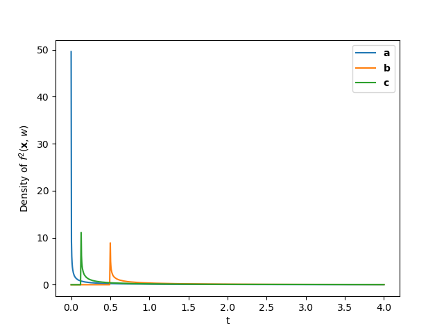
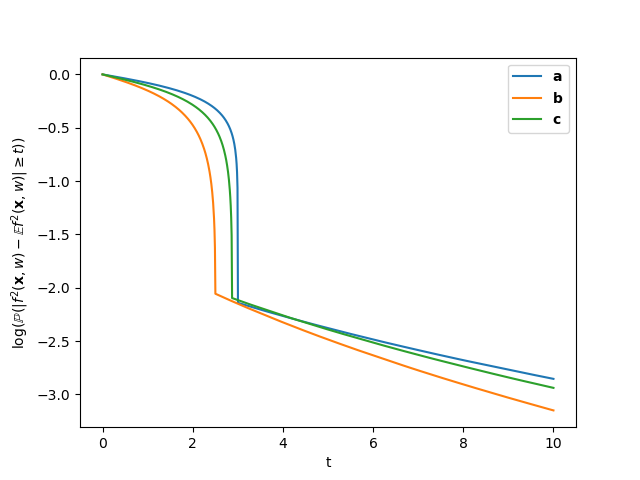
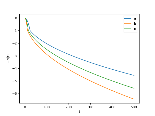
Figure 9. The left plot shows the density function of the squared distance $f^{2}(\mathbf{x},w)$ where $\mathbf{x}\in\{\mathbf{a},\mathbf{b},\mathbf{c}\}$ (as given in (24)) and $w$ is a standard Gaussian random variable. The plot in the middle displays the concentration behaviour of $f^{2}(\mathbf{x},w)$ around its mean (through the quantity $\log\mathbb{P}\left(|f^{2}(\mathbf{x},w)-\mathbb{E}f^{2}(\mathbf{x},w)|\geq t\right)$). The numerical values shown in these first two plots are simulated using a Monte Carlo method. Finally, the plot on the right shows the theoretical tail behaviour given by the bounds in Corollary 35 (i.e. $-\eta(t)$).

Finally, let us note that in the higher dimensional case, the bounds provided by Theorem 34 explicitly depend on the symmetry assumptions on the connectivity matrix $W$, not only through the value of the expectation $\mathbb{E}\|f(\mathbf{a},W)\|^{2}_{2}$, but also through the choice of the appropriate polynomial $P$ (recall that $G$ needs to have independent entries). Let us illustrate this with a concrete example.

Example 6.

We consider the simple case where $T=1$ and $W\in\mathbb{R}^{2\times 2}$. We easily compute in this case

$$\|f(\mathbf{a},W)\|^{2}_{2}=a_{0}^{2}\sum_{1\leq i,j,k\leq 2}W_{ij}W_{ik}+2a_{0}a_{1}\sum_{1\leq i,j\leq 2}W_{ij}+2a_{1}^{2}.$$

Assume that the entries of $W$ are i.i.d. centred Gaussian random variables with standard variation $\sigma>0$. The polynomial to consider is then

$$P(w_{11},w_{12},w_{21},w_{22})=a_{0}^{2}\sigma^{2}\sum_{1\leq i,j,k\leq 2}w_{ij}w_{ik}+2a_{0}a_{1}\sigma\sum_{1\leq i,j\leq 2}w_{ij}+2a_{1}^{2}.$$

Hence

$$\mathbb{E}P^{(1)}(w_{11},w_{12},w_{21},w_{22})=2a_{0}a_{1}\sigma(1,1,1,1)^{\top},$$

and $P^{(2)}(w_{11},w_{12},w_{21},w_{22})\in(\mathbb{R}^{4})^{\otimes 2}$ is given by

$$2a_{0}^{2}\sigma^{2}\left(\begin{array}[]{cccc}1&1&0&0\\ 1&1&0&0\\ 0&0&1&1\\ 0&0&1&1\\ \end{array}\right).$$

Therefore

$$\|\mathbb{E}P^{(2)}(w_{11},w_{12},w_{21},w_{22})\|_{\mathrm{op}}=4a_{0}^{2}\sigma^{2}\quad\text{and}\quad\|\mathbb{E}P^{(2)}(w_{11},w_{12},w_{21},w_{22})\|_{\mathrm{HS}}=4\sqrt{2}a_{0}^{2}\sigma^{2}.$$

Thus, $\log(\mathbb{P}(\|f(\mathbf{a},W)\|^{2}_{2}-\mathbb{E}\|f(\mathbf{a},W)\|^{2}_{2}\geq t))$ decays like

$$-\min\left(\left(\frac{t}{4a_{0}a_{1}\sigma}\right)^{2},\left(\frac{t}{4\sqrt{2}a_{0}^{2}\sigma^{2}}\right)^{2},\frac{t}{4a_{0}^{2}\sigma^{2}}\right).$$

Assume now that $W$ is symmetric with the entries on and above the diagonal being i.i.d. centred Gaussian random variables with standard variation $\sigma>0$. In this case, the polynomial to consider is

$$\begin{array}[]{rcl}Q(w_{11},w_{12},w_{22})&=&a_{0}^{2}\sigma^{2}(w_{11}^{2}+w_{22}^{2}+2w_{12}^{2}+2w_{11}w_{12}+2w_{12}w_{22})\\ &&+2a_{0}a_{1}\sigma(w_{11}+w_{22}+2w_{12})+2a_{1}^{2}.\\ \end{array}$$

Hence

$$\mathbb{E}Q^{(1)}(w_{11},w_{12},w_{22})=2a_{0}a_{1}\sigma(1,2,1)^{\top},$$

and $Q^{(2)}(w_{11},w_{12},w_{22})\in(\mathbb{R}^{3})^{\otimes 2}$ is given by the matrix

$$2a_{0}^{2}\sigma^{2}\left(\begin{array}[]{ccc}1&1&0\\ 1&2&1\\ 0&1&1\\ \end{array}\right).$$

Therefore

$$\|\mathbb{E}Q^{(2)}(w_{11},w_{12},w_{22})\|_{\mathrm{op}}=6a_{0}^{2}\sigma^{2}\quad\text{and}\quad\|\mathbb{E}Q^{(2)}(w_{11},w_{12},w_{22})\|_{\mathrm{HS}}=2\sqrt{10}a_{0}^{2}\sigma^{2}.$$

Thus, $\log(\mathbb{P}(\|f(\mathbf{a},W)\|^{2}_{2}-\mathbb{E}\|f(\mathbf{a},W)\|^{2}_{2}\geq t))$ decays like

$$-\min\left(\left(\frac{t}{2\sqrt{6}a_{0}a_{1}\sigma}\right)^{2},\left(\frac{t}{2\sqrt{10}a_{0}^{2}\sigma^{2}}\right)^{2},\frac{t}{6a_{0}^{2}\sigma^{2}}\right).$$

For the numerical simulations, we consider the sequence $\mathbf{a}=\left(\frac{b_{t}}{\|\mathbf{b}\|_{2}}\right)_{0\leq t\leq 5}$, where $\mathbf{b}=\left(\frac{(-1)^{t}}{(6-t)!}\right)_{0\leq t\leq 5}$. We plot the density and the tails of $\|f(\mathbf{a},W)\|^{2}_{2}$, with $W$ being an $N\times N$ random matrix that either has independent entries or is symmetric with independent entries on and above the diagonal. In both cases, the entries of $W$ are centred Gaussian of variance $\frac{1}{N}$. The results are shows in Figures 10 and 11.

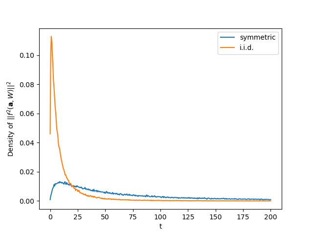
(a) $N=10$

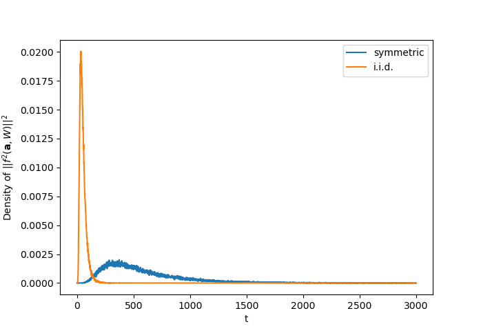
(b) $N=50$

Figure 10. Density function of $\|f(\mathbf{a},W)\|^{2}_{2}$, where $W$ is an $N\times N$ random matrix that either has independent entries or is symmetric with independent entries on and above the diagonal. The entries of $W$ are centred Gaussian of variance $\frac{1}{N}$.

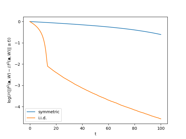
(a) $N=10$

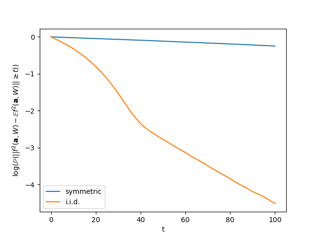
(b) $N=50$

Figure 11. Plot of the tail function $t\mapsto\log\mathbb{P}\left(|\|f(\mathbf{a},W)\|^{2}_{2}-\mathbb{E}\|f(\mathbf{a},W)\|^{2}_{2}|\geq t\right)$, where $W$ is an $N\times N$ random matrix that either has independent entries or is symmetric with independent entries on and above the diagonal. The entries of $W$ are centred Gaussian of variance $\frac{1}{N}$.

Both figures seem to indicate that the expected square distance between reservoir states is a better representative of the square distance (as a random variable) in the i.i.d. case than in the symmetric one. The lack of dispersion around the mean can be thought of as a consistency guarantee of separation of several time series at once.

References

- [AD19] Mathieu Alain and Nicolas Doyon. Les systèmes dynamiques de grande taille, un lien entre la réciprocité et le rayon spectral. Bulletin AMQ, 59(3), 2019.
- [AGZ10] Greg W Anderson, Alice Guionnet, and Ofer Zeitouni. An introduction to random matrices. Number 118. Cambridge university press, 2010.
- [ASVdS+11] Lennert Appeltant, Miguel Cornelles Soriano, Guy Van der Sande, Jan Danckaert, Serge Massar, Joni Dambre, Benjamin Schrauwen, Claudio R Mirasso, and Ingo Fischer. Information processing using a single dynamical node as complex system. Nature communications, 2(1):468, 2011.
- [AW15] Radosł aw Adamczak and PawełWolff. Concentration inequalities for non-Lipschitz functions with bounded derivatives of higher order. Probab. Theory Related Fields, 162(3-4):531–586, 2015.
- [Bai97] Zhi Dong Bai. Circular law. The Annals of Probability, 25(1):494–529, 1997.
- [BC85] Stephen Boyd and Leon O. Chua. Fading memory and the problem of approximating nonlinear operators with Volterra series. IEEE Trans. Circuits and Systems, 32(11):1150–1161, 1985.
- [BCI02] Christian Berg, Yang Chen, and Mourad EH Ismail. Small eigenvalues of large hankel matrices: The indeterminate case. Mathematica Scandinavica, pages 67–81, 2002.
- [BFS93] Y. Bengio, P. Frasconi, and P. Simard. The problem of learning long-term dependencies in recurrent networks. In IEEE International Conference on Neural Networks, pages 1183–1188 vol.3, 1993.
- [Bol13] Béla Bollobás. Modern graph theory, volume 184. Springer Science & Business Media, 2013.
- [BS11] Christian Berg and Ryszard Szwarc. The smallest eigenvalue of Hankel matrices. Constr. Approx., 34(1):107–133, 2011.
- [CG90] J Carnicer and M Gasca. Evaluation of multivariate polynomials and their derivatives. Mathematics of Computation, 54(189):231–243, 1990.
- [CGG+22] Christa Cuchiero, Lukas Gonon, Lyudmila Grigoryeva, Juan-Pablo Ortega, and Josef Teichmann. Discrete-time signatures and randomness in reservoir computing. IEEE Trans. Neural Netw. Learn. Syst., 33(11):6321–6330, 2022.
- [CLRS22] Thomas H Cormen, Charles E Leiserson, Ronald L Rivest, and Clifford Stein. Introduction to algorithms. MIT press, 2022.
- [DCR+18] Brian DePasquale, Christopher J Cueva, Kanaka Rajan, G Sean Escola, and LF Abbott. full-FORCE: A target-based method for training recurrent networks. PloS one, 13(2):e0191527, 2018.
- [DG03] Sanjoy Dasgupta and Anupam Gupta. An elementary proof of a theorem of Johnson and Lindenstrauss. Random Structures & Algorithms, 22(1):60–65, 2003.
- [DGJS22] Sjoerd Dirksen, Martin Genzel, Laurent Jacques, and Alexander Stollenwerk. The separation capacity of random neural networks. J. Mach. Learn. Res., 23:Paper No. [309], 47, 2022.
- [Doy92] Kenji Doya. Bifurcations in the learning of recurrent neural networks 3. learning (RTRL), 3:17, 1992.
- [GGO23] Lukas Gonon, Lyudmila Grigoryeva, and Juan-Pablo Ortega. Approximation bounds for random neural networks and reservoir systems. Ann. Appl. Probab., 33(1):28–69, 2023.
- [GGT23] Alexander Gorban, Bogdan Grechuk, and Ivan Tyukin. Stochastic separation theorems: how geometry may help to correct AI errors. Notices Amer. Math. Soc., 70(1):25–33, 2023.
- [GO18a] Lyudmila Grigoryeva and Juan-Pablo Ortega. Echo state networks are universal. Neural Networks, 108:495–508, 2018.
- [GO18b] Lyudmila Grigoryeva and Juan-Pablo Ortega. Universal discrete-time reservoir computers with stochastic inputs and linear readouts using non-homogeneous state-affine systems. Journal of Machine Learning Research, 19(24):1–40, 2018.
- [GO20] Lukas Gonon and Juan-Pablo Ortega. Reservoir computing universality with stochastic inputs. IEEE Trans. Neural Netw. Learn. Syst., 31(1):100–112, 2020.
- [GS20] Claudio Gallicchio and Simone Scardapane. Deep randomized neural networks. In Recent Trends in Learning From Data: Tutorials from the INNS Big Data and Deep Learning Conference (INNSBDDL2019), pages 43–68. Springer, 2020.
- [GSS21] Friedrich Götze, Holger Sambale, and Arthur Sinulis. Concentration inequalities for polynomials in -sub-exponential random variables. Electron. J. Probab., 26:Paper No. 48, 22, 2021.
- [Ham20] Hans Hamburger. Über eine Erweiterung des Stieltjesschen Momentenproblems. Mathematische Annalen, 81(2-4):235–319, 1920.
- [HD20] Moritz Helias and David Dahmen. Statistical field theory for neural networks, volume 970 of Lecture Notes in Physics. Springer, Cham, [2020] ©2020.
- [HP91] Peter Hilton and Jean Pedersen. Catalan numbers, their generalization, and their uses. The mathematical intelligencer, 13:64–75, 1991.
- [HS97] Sepp Hochreiter and Jürgen Schmidhuber. Long short-term memory. Neural computation, 9(8):1735–1780, 1997.
- [Hwa04] Suk-Geun Hwang. Cauchy’s interlace theorem for eigenvalues of hermitian matrices. The American mathematical monthly, 111(2):157–159, 2004.
- [JGP+19] Li Jing, Caglar Gulcehre, John Peurifoy, Yichen Shen, Max Tegmark, Marin Soljacic, and Yoshua Bengio. Gated orthogonal recurrent units: On learning to forget. Neural computation, 31(4):765–783, 2019.
- [JH04] Herbert Jaeger and Harald Haas. Harnessing nonlinearity: Predicting chaotic systems and saving energy in wireless communication. Science, 304(5667):78–80, 2004.
- [JL84] William B. Johnson and Joram Lindenstrauss. Extensions of Lipschitz mappings into a Hilbert space. In Conference in modern analysis and probability (New Haven, Conn., 1982), volume 26 of Contemp. Math., pages 189–206. Amer. Math. Soc., Providence, RI, 1984.
- [Lat06] Rafał Latała. Estimates of moments and tails of Gaussian chaoses. The Annals of Probability, 34(6):2315 – 2331, 2006.
- [LHEL21] Zhong Li, Jiequn Han, Weinan E, and Qianxiao Li. On the curse of memory in recurrent neural networks: Approximation and optimization analysis. In International Conference on Learning Representations, 2021.
- [LKDB18] Floris Laporte, Andrew Katumba, Joni Dambre, and Peter Bienstman. Numerical demonstration of neuromorphic computing with photonic crystal cavities. Opt. Express, 26(7):7955–7964, Apr 2018.
- [MJS07] Wolfgang Maass, Prashant Joshi, and Eduardo D Sontag. Computational aspects of feedback in neural circuits. PLoS Comput Biol, 3(1):e165, 2007.
- [SCS88] H. Sompolinsky, A. Crisanti, and H.-J. Sommers. Chaos in random neural networks. Phys. Rev. Lett., 61(3):259–262, 1988.
- [SH06] M.D. Skowronski and J.G. Harris. Minimum mean squared error time series classification using an echo state network prediction model. In 2006 IEEE International Symposium on Circuits and Systems, pages 4 pp.–3156, 2006.
- [ST50] James Alexander Shohat and Jacob David Tamarkin. The problem of moments, volume 1. American Mathematical Society (RI), 1950.
- [Sze36] Gabriel Szegö. On some Hermitian forms associated with two given curves of the complex plane. Trans. Amer. Math. Soc., 40(3):450–461, 1936.
- [Tin20] Peter Tino. Dynamical systems as temporal feature spaces. J. Mach. Learn. Res., 21:Paper No. 44, 42, 2020.
- [TV08] Terence Tao and Van Vu. Random matrices: the circular law. Communications in Contemporary Mathematics, 10(02):261–307, 2008.
- [VALT22] Pietro Verzelli, Cesare Alippi, Lorenzo Livi, and Peter Tiňo. Input-to-state representation in linear reservoirs dynamics. IEEE Trans. Neural Netw. Learn. Syst., 33(9):4598–4609, 2022.
- [Ver18] Roman Vershynin. High-dimensional probability, volume 47 of Cambridge Series in Statistical and Probabilistic Mathematics. Cambridge University Press, Cambridge, 2018. An introduction with applications in data science, With a foreword by Sara van de Geer.
- [VMVV+14] Kristof Vandoorne, Pauline Mechet, Thomas Van Vaerenbergh, Martin Fiers, Geert Morthier, David Verstraeten, Benjamin Schrauwen, Joni Dambre, and Peter Bienstman. Experimental demonstration of reservoir computing on a silicon photonics chip. Nature communications, 5(1):3541, 2014.
- [VSP+17] Ashish Vaswani, Noam Shazeer, Niki Parmar, Jakob Uszkoreit, Llion Jones, Aidan N Gomez, Łukasz Kaiser, and Illia Polosukhin. Attention is all you need. Advances in neural information processing systems, 30, 2017.
- [Wig55] Eugene P. Wigner. Characteristic vectors of bordered matrices with infinite dimensions. Annals of Mathematics, 62(3):548–564, 1955.
- [Yap00] Chee Keng Yap. Fundamental problems of algorithmic algebra. Oxford University Press, New York, 2000.