REFINED DISTRIBUTIONAL LIMIT THEOREMS
FOR COMPOUND SUMS

Vsevolod K. Malinovskii Central Economics and Mathematics Institute (CEMI) of Russian Academy of Science, 117418, Nakhimovskiy prosp., 47, Moscow, Russia admin@actlab.ru http://www.actlab.ru
Abstract.

The paper is a sketch of systematic presentation of distributional limit theorems and their refinements for compound sums. When analyzing, e.g., ergodic semi–Markov systems with discrete or continuous time, this allows us to separate those aspects that lie within the theory of random processes from those that relate to the classical summation theory. All these limit theorems are united by a common approach to their proof, based on the total probability rule, auxiliary multidimensional limit theorems for sums of independent random vectors, and (optionally) modular analysis.

Key words and phrases:
Compound sums, Clustering–type and queuing–type models, Distributional limit theorems, Refined approximations, Modular analysis, Renewal theory, Risk theory, ergodic Markov and semi–Markov systems.

1. Introduction

In his review [46] of Petrov’s book [80], Kesten111Harry Kesten (1931–2019), the Goldwin Smith Professor Emeritus of Mathematics, “whose insights advanced the modern understanding of probability theory and its applications” (quoted from obituary by Matt Hayes). wrote that “in the period 1920–1940 research in probability theory was virtually synonymous with the study of sums of independent random variables”, but “already in the late thirties attention started shifting and probabilists became more interested in Markov chains, continuous time processes, and other situations in which the independence between summands no longer applies, and today the center of gravity of probability theory has moved away from sums of independent random variables.”

Nevertheless, Kesten continues, “much work on sums of independent random variables continues to be done, partly for their aesthetic appeal and partly for the technical reason that many limit theorems, even for dependent summands, can be reduced to the case of independent summands by means of various tricks. The best known of these tricks is the use of regeneration points, or ‘Dœblin’s trick’. In large part the fascination of the subject is due to the fact that applications and the ingenuity of mathematicians continue to give rise to new questions.” Regarding applications, Kesten mentioned renewal theory, the theory of optimal stopping, invariance principles and functional limit theorems, fluctuation theory, and so on.

To summarize, Kesten argues that “in all the years that these newer phenomena were being discovered, people also continued working on more direct generalizations and refinements of the classical limit theorems $\dots$ Many of the proofs require tremendous skill in classical analysis $\dots$ and many of the results, such as the Berry–Esseen estimate, the Edgeworth expansion and asymptotic results for large deviations, are important for statistics and theoretical purposes.”

The paper is an overview that fits into the scheme outlined by Kesten. It is focussed on refined “distributional” (or “intrinsically analytic”222The terms “intrinsically analytic” and “measure–theoretic” applied to limit theorems are introduced in [19]. The former is equivalent (see, e.g., [12]) to “distributional”, or “weak”., or “weak”) limit theorems for compound sums which are a natural extension of ordinary sums. They are known as the key object of renewal theory and the core component of Dœblin’s dissection of an ordinary sum defined on a Markov chain. By “refined” limit theorems we mean333The results for large deviations, although interesting and available, are not presented here due to the space limitation. Berry–Esseen’s estimates and Edgeworth’s expansions mentioned by Kesten, in contrast to approximations without assessing their accuracy.

In contrast to “measure–theoretic” limit theorems, for which Kolmogorov’s axiomatization is indispensable and which border on (or lie within) the theory of random processes, “distributional” limit theorems, including those for dependent random variables, are known long before the axiomatization. For example, seeking in the 1900s, long before Kolmogorov’s advance, to demonstrate that independence is not a necessary condition in “distributional” weak law of large numbers (WLLN) and central limit theorem (CLT), Markov introduced the Markov chains.

Without questioning the value of “measure–theoretic” limit theorems, such as the strong law of large numbers (SLLN) and the law of iterated logarithm (LIL), or, going further, the value of the theory of random processes, we note that “distributional” rather than “measure–theoretic” limit theorems are really needed for statistics, cluster analysis, etc., where an infinite number of observations, clusters, renewals, people in queue, and so on, never occur. Even in Bernoulli’s classical scheme, statistical inference is based (see detailed discussion in [18]) on WLLN and CLT with its refinements, and not on SLLN and LIL.

Dealing with complex compound sums444See classification of compound sums below. Modular analysis is not needed for simple compound sums., we focus on modular analysis. Speaking of “Dœblin’s trick” which reduces “many limit theorems, even for dependent summands” to the case of independent ones, Kesten meant this approach. Bearing in mind the ladder technique, say “Blackwell’s trick” (see [13]), the modular analysis is even more widely used. We will expand it to compound sums with general modular structure, but note that (see, e.g., [39], [42], [65], [83], [87]) this is merely one, rather than the only and the best, method for studying such sums.

Technically, “Dœblin’s trick” (or its counterpart “Blackwell’s trick”) is not only the use of regeneration (or ladder) points. It implies (see, e.g., [20]) the use of Kolmogorov’s inequality for maximum of partial sums in order to move from Dœblin’s (or Blackwell’s) dissection to ordinary sum of independent modular summands. We call this approach “basic technique”.

Delving deeper, the “basic technique” in its original form fails in local theorems and yields no “refined” approximations, such as Berry–Esseen’s estimates and Edgeworth’s expansions. To be specific, dealing with a local limit theorem for classical Markov chains, Kolmogorov (see [49]) pointed that “Dœblin’s method in its original form” is suitable “only for proving integral theorems”. We quote555In our translation from Russian. Apparently, this article has not been translated in due course from Russian into English. more from [49], § 2: “$\dots$ the local theorems that form the main content of the present paper will be obtained $\dots$ with the help of some strengthening of the method that was developed by Dœblin for proving the integral limit theorem in the case of an infinite number of states. In order to make the development of the method clear, we single out $\dots$ a brief exposition of Dœblin’s method in its original form, in which it is suitable only for proving integral theorems.”

In brief, Kolmogorov’s advance in [49] was due to a straightforward use of the total probability formula, or, according to his terminology, “basic identity”.

Further progress was made thirty years later in [14] and in a series of papers (see, e.g., [15], [43], [55][60]) that followed: Berry–Esseen’s estimates and Edgeworth’s expansions in CLT for recurrent Markov chain were obtained by using the total probability rule and the auxiliary multidimensional limit theorems for sums of independent random vectors. To distinguish this approach from “basic technique”, or “Dœblin’s method in its original form”, we call it “advanced (modular, if switching to modular summands is needed) technique”.

Being one of the main pillars of the advanced technique, the limit theorems for sums of independent random vectors (see, e.g., [11], [31][33]) are close to perfection. In the advanced technique, analytical complexity, which never disappears but flows from one form to another, is split into the use of, firstly, the auxiliary theorems where (we quote from Preface of [11]) “precision and generality go hand in hand” and, secondly, tedious but fairly standard classical analysis, e.g., approximation of integral sums by appropriate integrals and evaluation of remainder terms.

Further presentation is arranged as follows. Section 2 is devoted to genesis and classification of compound sums. In Section 3, we address elementary and refined renewal theorems and refined limit theorems for cumulated rewards. Having formulated them as limit theorems for simple compound sums, we outline their proof using advanced technique instead of renewal equation, Laplace transforms, and Tauberian theorems commonly used in renewal theory.

In Section 4, we address complex compound sums “with irregular summation and independence” related to the ruin problem of collective risk theory. To get (refined) normal approximation when such sums are proper, we use the modular analysis based on Blackwell’s ladder idea. To get (refined) quasi–normal approximation when such sums are defective, we resort to associated random variables. In this context, we touch upon the inverse Gaussian approximation which deviates somewhat from the main topic of this paper, but demonstrates that there are more sophisticated methods than those related to asymptotic normality.

In Section 5, seeking to use the full force of modular analysis combined with advanced technique, we focus on compound sums with general modular structure. Particular cases of this framework are complex compound sums “with irregular summation and dependence”, in particular Markov dependence. The only case, although of significant practical interest, where great impediments for asymptotic analysis arise is defective compound sums “with irregular summation and dependence”. This case, which is tackled by means of computer–intensive analysis, is briefly discussed in Section 6. A concluding remark is made in Section 7.

The article, being a review, does not contain complete proofs. Most results are formulated in a non–strict manner, although the necessary references are given everywhere. Striving for clarity, great emphasis is placed on discussing the main ideas of the proofs. Overall, the aims of the advance described in this review are the same as Loève stated in [53] writing on limit theorems of probability theory: (i) to simplify proofs and forge general tools out of the special ones, (ii) to sharpen and strengthen results, (iii) to find general notions behind the results obtained and to extend their domains of validity.

2. Genesis and classification of compound sums

It was observed (see [69]) that “on the Continent, if people are waiting at a bus–stop, they loiter around in a seemingly vague fashion. When the bus arrives, they make a dash for it $\dots$ An Englishman, even if he is alone, forms an orderly queue of one.” In terms of mathematical modeling, this is a “clustering–type” model opposed to a “queuing–type” model. In the former, there is essentially no flow of time, and the objects or events of interest are scattered in space. In the latter, there is a flow of time, and the objects or events of interest form an ordered queue.

In models of both types, the core is the compound sum

$${S}_{N_{t}}=\sum_{i=1}^{N_{t}}X_{i}$$

with basis $(T_{i},X_{i})$, $i=1,2,\dots$, where $t>0$ and

$$N_{t}=\inf\Big{\{}n\geqslant 1:\sum_{i=1}^{n}T_{i}>t\Big{\}}$$ (2.1)

or $+\infty$, if the set is empty666Recall that $\inf\emptyset=+\infty$, $\sup\emptyset=0$.. When $N_{t}=+\infty$, the sum ${S}_{N_{t}}$ is set equal to $+\infty$. For brevity, the real–valued random variables $X_{i}$ are called primary components ($p$–components) and $T_{i}$ secondary components ($s$–components) of the basis.

If the basis $(T_{i},X_{i})$, $i=1,2,\dots$, consists of independent random vectors, then ${S}_{N_{t}}$ is “with independence”. Otherwise it is “with dependence”. Examples of the latter are often found (see, e.g., [78]) in various models with Markov modulation. If $s$–components are positive, then ${S}_{N_{t}}$ is “with regular summation”. Otherwise, it is “with irregular summation”.

Apparently, compound sums “with regular summation and independence” fully and distinctly came forth in “queuing–type” renewal theory and its ramifications. Compound sums “with irregular summation and independence” appeared (see, e.g., [66]) in ruin problem and (see, e.g., [41]) in many settings which involve random walks. On the other hand, Dœblin’s dissection, i.e., switching from ordinary sum defined on a Markov chain to modular simple compound sum “with regular summation and independence”, whose basis consists of intervals between regeneration points and increments at these intervals, is another source of compound sums.

The complexity of “irregular summation” is rather transparent: the sums ${V}_{n}=\sum_{i=1}^{n}T_{i}$, $n=1,2,\dots$, are not progressively increasing, whence $\{N_{t}=n\}$ is equal to $\{{V}_{1}\leqslant t,\dots,{V}_{n-2}\leqslant t,{V}_{n-1}\leqslant t<{V}_{n}\}$, rather than $\{{V}_{n-1}\leqslant t<{V}_{n}\}$, as would be for “regular summation”.

In “dependence complexity” case, the model has to be fleshed out. In the search of non–trivial examples which illustrate the general results, we focus on Markov dependence and its extensions, but in fact any type of dependence which allows an embedded modular structure with independent modules suits us well. In terms of random processes, much of this topic is based on successive “starting over”, as time goes on, commonly called “regeneration” or (see [47], [78]) “regenerative phenomena”. With this approach, many cases that go beyond the scope of Markov theory fall within the scope of this paper.

Remark 2.1.

Beyond the scope of this paper are the sums of the following two types. First, the random sums ${S}_{N}$ with $N$ and $X_{1},X_{2},\dots$ not necessarily independent of each other, but with $N$ not of the form (2.1) or the similar. Second, the random sums ${S}_{N}=\sum_{i=1}^{N}X_{i}$ with independence between $N$ and $X_{1},X_{2},\dots$. The former were introduced in [6], [81], [82], and investigated, e.g., in [41]. The latter were introduced in [84] and thoroughly studied (see, e.g., [38]) in many works.∎

2.1. Proper and defective compound sums

{bundle}

Compound sum \chunk $\mathcal{R\hskip-0.5pt/I}$  sum \chunk{bundle} $\mathcal{I\hskip-0.5pt/I}$  sum \chunk proper $\mathcal{I\hskip-0.5pt/I}$  sum \chunk defective $\mathcal{I\hskip-0.5pt/I}$  sum \chunk $\mathcal{R\hskip-0.5pt/D}$  sum \chunk{bundle} $\mathcal{I\hskip-0.5pt/D}$  sum \chunk proper $\mathcal{I\hskip-0.5pt/D}$  sum \chunk defective $\mathcal{I\hskip-0.5pt/D}$  sum

Figure 1. Classification of compound sums.

The classification of compound sums, where shorthand for “compound sum with regular summation and independence” is “$\mathcal{R\hskip-0.5pt/I}$  sum”, for “compound sum with irregular summation and independence” is “$\mathcal{I\hskip-0.5pt/I}$  sum”, for “compound sum with regular summation and dependence” is “$\mathcal{R\hskip-0.5pt/D}$  sum”, and for “compound sum with irregular summation and dependence” is “$\mathcal{I\hskip-0.5pt/D}$  sum”, is shown in Fig. 1. Under natural regularity conditions, compound sums “with regular summation” are always proper, while compound sums “with irregular summation” are either proper, or defective777Recall (see [37]) that a random variable is defective, with defect $1-p$, if it takes the value $\infty$ with probability $p>0$. Otherwise, it is proper..

The following example shows that finding the defect of $\mathcal{I\hskip-0.5pt/I}$  sum is not easy.

Example 2.1.

Let $(X_{i},Y_{i})$, $i=1,2,\dots$, be a subsidiary sequence of i.i.d.  random vectors, whose components are positive and independent of each other. For $c>0$ and $T_{i}=Y_{i}-cX_{i}$, ${S}_{N_{t}}=\sum_{i=1}^{N_{t}}X_{i}$ is positive $\mathcal{I\hskip-0.5pt/I}$  sum with basis $(T_{i},X_{i})$, $i=1,2,\dots$. While the components of the subsidiary sequence are independent of each other, the components of the basis are dependent on each other. If $X_{i}$ and $Y_{i}$, $i=1,2,\dots$, are exponentially distributed with positive parameters $\varrho$ and $\rho$, then (see, e.g., [65], Theorem 5.8)

$$\mathsf{P}\big{\{}{S}_{N_{t}}\leqslant x\big{\}}=\mathsf{P}\big{\{}{S}_{N_{t}}<\infty\big{\}}-\frac{1}{\pi}\int_{0}^{\pi}f(z,t,x)\,dz,$$ (2.2)

where

$$\mathsf{P}\big{\{}{S}_{N_{t}}<\infty\big{\}}=\begin{cases}1,&\varrho/(c\rho)\geqslant 1,\\[8.0pt] \dfrac{\varrho}{c\rho}\,\exp\big{\{}-t(c\rho-\varrho)/c\big{\}},&\varrho/(c\rho)<1\end{cases}$$ (2.3)

and

$\displaystyle f(z,t,x)=$ $\displaystyle\,(\varrho/(c\rho))(1+\varrho/(c\rho)-2\sqrt{\varrho/(c\rho)}\cos z)^{-1}$ (2.4)
$\displaystyle\times\exp\big{\{}t\rho\,(\sqrt{\varrho/(c\rho)}\cos z-1)$
$\displaystyle-x\varrho(c\rho/\varrho)(1+\varrho/(c\rho)-2\sqrt{\varrho/(c\rho)}\cos z)\big{\}}$
$\displaystyle\times(\cos(t\rho\sqrt{\varrho/(c\rho)}\sin z)-\cos(t\rho\sqrt{\varrho/(c\rho)}\sin z+2z)).$

Consequently, ${S}_{N_{t}}$ is proper if $\varrho/(c\rho)\geqslant 1$, which is equivalent to $c\leqslant c^{\ast}=\mathsf{E}{Y}/\mathsf{E}{X}$, and defective otherwise. Defect of ${S}_{N_{t}}$ is yielded in (2.3). ∎

Although the expression (2.3) for defect of ${S}_{N_{t}}$ is complicated888This is a particular case of Cramér’s famous result on the probability of ultimate ruin., the conditions under which ${S}_{N_{t}}$ is proper or defective, are simple. On the one hand, if $\mathsf{E}T_{1}>0$, then (see Theorem 2 in [37], Chapter XII) the ordinary sums ${V}_{n}$ increase a.s.  to $+\infty$, as $n\to\infty$. Consequently, for any $t$ the summation limit $N_{t}$ is a.s.  finite and ${S}_{N_{t}}$ is a.s.  less than $+\infty$, whence proper. On the other hand, if $\mathsf{E}T_{1}<0$, then the ordinary sums ${V}_{n}$ decrease a.s.  to $-\infty$, as $n\to\infty$. With a positive probability, the maximum $M=\max_{n\in\mathsf{N}}{V}_{n}$ is finite and less than $t>0$ large enough, whence $N_{t}$ and ${S}_{N_{t}}$ are defective.

2.2. Renewal theory and species of compound sums

In renewal theory, $p$–components $X_{i}$, $i=1,2,\dots$, (typically positive) are called “rewards in the moments of renewals” and $s$–components $T_{i}$, $i=1,2,\dots$, (always positive) are called “intervals between successive renewals”. This interpretation yields a variety of species of $\mathcal{R\hskip-0.5pt/I}$  sums. In particular, the total number of renewals before time $t$, defined as $\widetilde{N}_{t}=\sup\{n\geqslant 1:{V}_{n}\leqslant t\}$, or 00, if $T_{1}>t$, comes to the fore. Focus shifts from $N_{t}$ to $\widetilde{N}_{t}$, which coincides with $\widehat{N}_{t}=N_{t}-1$ trivially related to $N_{t}$.

When moving from relatively simple $\mathcal{R\hskip-0.5pt/I}$  sums to more complicated $\mathcal{I\hskip-0.5pt/I}$ and $\mathcal{I\hskip-0.5pt/D}$  sums, both of them with “irregular summation”, the difference between altered (with summation limit $\widetilde{N}_{t}$) and non–altered (with summation limit $N_{t}$) compound sums becomes non–trivial: $\widetilde{N}_{t}$ is no more trivially related to $N_{t}$ and the altered compound sums ${S}_{\widetilde{N}_{t}}=\sum_{i=1}^{\widetilde{N}_{t}}X_{i}$ and ${S}_{\widehat{N}_{t}}=\sum_{i=1}^{\widehat{N}_{t}}X_{i}$ are not bounded to coincide.

As for $\mathcal{R\hskip-0.5pt/D}$  sums with Markov dependence, which generalize $\mathcal{R\hskip-0.5pt/I}$  sums in the same way as Markov renewal theory generalizes renewal theory, dependence is introduced by embedded Markov chain $\{\xi_{i}\}_{i\geqslant 0}$. In such $\mathcal{R\hskip-0.5pt/D}$  sums, $s$–components $T_{i}$, $i=1,2,\dots$, are the time intervals between jumps of $\{\xi_{i}\}_{i\geqslant 0}$ and $p$–components $X_{i}$, $i=1,2,\dots$, which depend on $\{\xi_{i}\}_{i\geqslant 0}$, are rewards in the moments of renewals.

In this way, the variety of species of compound sums echoes the diversity of renewal processes. There are999We refer to [21], Section 2.2, or [22], Section 9.2. There are terminological collisions, e.g., in [45], Chapter 5, Section 7, this process is called delayed renewal process. modified, equilibrium, and ordinary renewal processes. If $T_{1}$ is distributed differently than $T_{i}\overset{d}{=}T$, $i=2,3,\dots$, then the renewal process is called modified. When all intervals between renewals, including the first one, are identically distributed, the renewal process is called ordinary. Furthermore, if

$$\mathsf{P}\big{\{}T_{1}\leqslant x\big{\}}=\frac{1}{\mathsf{E}T}\int_{0}^{x}\big{(}1-F_{T}(z)\big{)}\,dz,\quad x>0,$$

where $F_{T}$ denotes c.d.f.  of $T$, then it is called equilibrium, or stationary.

Regarding compound sums, modified are those in which a finite number of elements of the basis $(T_{i},X_{i})$, $i=1,2,\dots$, e.g., the first element $(T_{1},X_{1})$, differ from all the others. Unlike in renewal theory which models technical repairable systems where the first repair does not necessarily occur at the starting time zero, this modification looks awkward for $\mathcal{R\hskip-0.5pt/I}$  sums: it boils down to a very special case of non–identically distributed summands. The similar modification of $\mathcal{R\hskip-0.5pt/D}$  sums with Markov dependence comes down to the choice of the initial distribution of the embedded Markov chain $\{\xi_{i}\}_{i\geqslant 0}$ and is much more sensible.

It is noteworthy that, under natural regularity conditions, switching within the species of compound sums, e.g., from altered to unaltered compound sums and vice versa, does not affect the main–term approximations, but affects refinements such as Edgeworth’s expansions.

3. Renewal theory and limit theorems for $\boldsymbol{\mathcal{R\hskip-0.5pt/I}}$  sums

Founded (see [34], [35]) in the 1940s as a theoretical insight into technical repairable systems, the classical renewal theory is focussed on “queuing–type” models. The term “renewal”, which displaced the formerly used term “industrial replacement” coined (see [54]) in the 1930s by Lotka, is widely used nowadays, but was not the main or default term even in Feller’s seminal paper [36] dated 1949.

In 1948, Doob [30] noted that “renewal theory is ordinarily reduced to the theory of certain types of integral equations $\dots$ However, it is to be expected that a treatment in terms of the theory of probability, which uses the modern developments of this theory, will shed new light on the subject.” Feller agreed (see [37], Chapter VI) that in renewal theory “analytically, we are concerned merely with sums of independent positive variables.”

3.1. First appearance of the advanced technique

In words, the renewal function101010The asterisk denotes the convolution operator. $\mathsf{U}(t)=\sum_{n=0}^{\infty}F_{T}^{*n}(t)$, $t>0$, where $F_{T}$ denotes c.d.f.  of a positive random variable $T$, is the expected number of renewals in the time interval $(0,t)$, with the origin counted as renewal epoch111111In [22], [45], the renewal function is defined as $\mathsf{H}(t)=\mathsf{U}(t)-1$, $t>0$ (or $\mathsf{E}\widehat{N}_{t}$), which differs from $\mathsf{U}(t)$ by one. In [37], the function $\mathsf{U}(t)$, $t>0$, is called the (ordinary) renewal process. In [22], [45], the renewal process is referred to as the continuous–time random process $\{\widehat{N}_{t}\}_{t\geqslant 0}$, i.e., the random number of renewals in the time interval $(0,t)$, with the origin not being counted as a renewal epoch.. As a formula, this is $\mathsf{U}(t)=1+\mathsf{E}\widehat{N}_{t}$. Together with altered $\mathcal{R\hskip-0.5pt/I}$  sum ${S}_{\widehat{N}_{t}}$, called in renewal theory “cumulated rewards”, it is built on $\mathcal{R\hskip-0.5pt/I}$  basis $(T_{i},X_{i})\overset{d}{=}(T,X)$, $i=1,2,\dots$, with i.i.d.  components and $T$ positive.

The elementary renewal theorem (see, e.g., [41]), states that for $0<\mathsf{E}\,T\leqslant\infty$ the approximation121212When $\mathsf{E}\,T=\infty$, the ratio $t/\mathsf{E}\,T$ is replaced by 00.

$$\mathsf{E}\widehat{N}_{t}=\frac{t}{\mathsf{E}\,T}+o(t),\quad t\to\infty,$$ (3.1)

holds. The corresponding expansion up to vanishing term is

$$\mathsf{E}\widehat{N}_{t}=\frac{t}{\mathsf{E}\,T}+\frac{\mathsf{D}T-(\mathsf{E}\,T\,)^{2}}{2\,(\mathsf{E}\,T\,)^{2}}+o(1),\quad t\to\infty,$$ (3.2)

called refined elementary renewal theorem.

The elementary renewal theorem is widely known: see, e.g., Equality (3) in [21], Section 4.2, or Equality (17) in [22], Section 9.2, or main formula in point (b) in [45], Chapter 5, Section 6. In [22], p. 345, it is noted that “a rigorous proof $\dots$ is possible under very weak assumptions about the distribution of $T$, but requires difficult Tauberian arguments and will not be attempted here”. It can also be obtained (with some caution with regard to the definition of renewal function) from Theorem 1 in [37], Chapter XI, the proof of which is based on the renewal equation.

The refined elementary renewal theorem and the similar results for higher–order power moments of $\widehat{N}_{t}$ and ${S}_{\widehat{N}_{t}}$, including expansions up to vanishing terms, were studied (see, e.g., [21], Section 4.5, and [3]) by various methods.

We outline a proof (see details in [65], Chapter 4) that does not compete with the proofs mentioned above in the sense of elegance or minimality of conditions. The advantage of this proof, based on the use of refined CLT and consisting of steps  A–F, is that it will be routinely carried over to much more complex settings.

Step  A:  use of fundamental identity.  The identity

$\displaystyle\mathsf{E}\widehat{N}_{t}=$ $\displaystyle\,\sum_{n=1}^{\infty}n\;\mathsf{P}\big{\{}\widehat{N}_{t}=n\big{\}}=\sum_{n=1}^{\infty}n\;\mathsf{P}\bigg{\{}\sum_{i=1}^{n}T_{i}\leqslant t<\sum_{i=1}^{n+1}T_{i}\bigg{\}}$ (3.3)
$\displaystyle=$ $\displaystyle\,\sum_{n=1}^{\infty}n\big{(}F_{T}^{*n}(t)-F_{T}^{*(n+1)}(t)\big{)}$

is obvious. If the probability density function (p.d.f.) $f_{T}$ exists (we assume this for simplicity of presentation), then (3.3) can be rewritten as

$\displaystyle\mathsf{E}\widehat{N}_{t}=\sum_{n=1}^{\infty}n\int_{0}^{t}f_{T}^{*n}(t-z)\,\mathsf{P}\big{\{}T_{n+1}>z\big{\}}\,dz.$ (3.4)

Step  B:  reduction of range of summation.  At this step, we cut out from the sum on the right side of (3.3) those terms that correspond to small $n$ (i.e., $n<n_{t}$ with properly selected $n_{t}\to\infty$, as $t\to\infty$). This is intuitively clear: for large $t$, the random variable $\widehat{N}_{t}$ is likely to be large. Therefore, the probabilities $\mathsf{P}\big{\{}\widehat{N}_{t}=n\big{\}}$ for small $n$ are small. Technically, it is done using the well–known probability inequalities, such as Markov’s inequality.

Step  C:  reduction of range of integration.  At this step, relying on the moment conditions, we cut out from the integral in (3.4) that part that corresponds to large $z$ (i.e., $z>z_{t}$ with properly selected $z_{t}\to\infty$, as $t\to\infty$). This is also intuitively clear: any single random variable, including $T_{n+1}$, is small compared to the sum $\sum_{i=1}^{n}T_{i}$, as $n$ is sufficiently large.

Step  D:  application of refined CLT.  Writing $\mu_{T}=\mathsf{E}\,T$, $\sigma_{T}^{2}=\mathsf{D}\,T$ and switching to standardized random variables $\tilde{T}_{i}=(T_{i}-\mu_{T})/\sigma_{T}$, $i=1,2,\dots$, we have

$$f_{T}^{*n}(t-z)=\frac{1}{\sigma_{T}\sqrt{n}}\,f_{\,n^{-1/2}\sum_{i=1}^{n}\tilde{T}_{i}}\big{(}\lambda_{T,n}{(t-z)}\big{)},$$

where $\lambda_{T,n}{(t-z)}=(t-z-\mu_{T}n)/(\sigma_{T}\sqrt{n})$. Assuming that natural moment conditions are satisfied, we apply Berry–Esseen’s estimate (see Theorem 11 in [80], Chapter VII, § 2) in the proof of (3.1) and Edgeworth’s expansion (see Theorem 17 in [80], Chapter VII, § 3) in the proof of (3.2). In both cases, these results are taken with non–uniform remainder terms.

Step  E:  analysis of approximating term.  In the proof of (3.1), where Berry–Esseen’s estimate was used, the approximating term is

$$\mathcal{I}_{t}=\frac{1}{\sigma_{T}}\sum_{n>n_{t}}n^{1/2}\int_{0}^{z_{t}}\varphi_{\left({0},{1}\right)}\big{(}\lambda_{T,n}{(t-z)}\big{)}\,\mathsf{P}\big{\{}T>z\big{\}}\,dz,$$

where $\varphi_{\left({0},{1}\right)}$ denotes p.d.f.  of standard normal distribution. In the proof of (3.2), where Edgeworth’s expansion was used, the approximating term is the sum of

$\displaystyle\mathcal{I}_{t}^{\,{\dagger}}=$ $\displaystyle\,\frac{1}{\sigma_{T}}\sum_{n>n_{t}}\sqrt{n}\int_{0}^{z_{t}}\varphi_{\left({0},{1}\right)}(\lambda_{T,n}{(t-z)})\,\mathsf{P}\big{\{}T>z\big{\}}\,dz$
$\displaystyle\mathcal{I}_{t}^{\,{\ddagger}}=$ $\displaystyle\,\frac{1}{\sigma_{T}}\frac{\mathsf{E}(T^{3})}{6\,\sigma_{T}^{3}}\sum_{n>n_{t}}\int_{0}^{z_{t}}\,\big{(}\lambda_{T,n}^{3}{(t-z)}-3\,\lambda_{T,n}{(t-z)}\big{)}$
$\displaystyle\times\varphi_{\left({0},{1}\right)}\big{(}\lambda_{T,n}{(t-z)}\big{)}\,\mathsf{P}\big{\{}T>z\big{\}}\,dz.$

Using Riemann summation formula with nodal points $\lambda_{T,n}{(t)}{}<\lambda_{T,n-1}{(t)}{}<\dots<\lambda_{T,2}{(t)}{}<\lambda_{T,1}{(t)}{}$, we seek to reduce $\mathcal{I}_{t}$ to ${t}/{\mathsf{E}\,T}$ with the required accuracy, and $\mathcal{I}_{t}^{\,{\dagger}}+\mathcal{I}_{t}^{\,{\ddagger}}$ to $t/\mathsf{E}\,T+(\mathsf{D}T-(\mathsf{E}\,T)^{2})/(2\,(\mathsf{E}\,T)^{2})$ with the required accuracy. This is a tedious but fairly standard classical analysis left to the reader.

Step  F:  analysis of remainder term.  In the proof of (3.1), the remainder term is

$$\mathcal{R}_{t}={C}_{1}\sum_{n>n_{t}}\delta_{n}\int_{0}^{z_{t}}\big{(}1+|\,\lambda_{T,n}{(t-z)}\,|\,\big{)}^{-3}\,\mathsf{P}\big{\{}T>z\big{\}}\,dz.$$

In the proof of (3.2), the remainder term is

$\displaystyle\mathcal{R}_{t}=$ $\displaystyle\,{C}_{2}\sum_{n>n_{t}}\frac{\delta_{n}}{\sqrt{n}}\int_{0}^{z_{t}}\big{(}1+\big{|}\,\lambda_{T,n}{(t-z)}\,\big{|}\,\big{)}^{-4}\,\mathsf{P}\big{\{}T>z\big{\}}\,dz,$

with $\delta_{n}\to 0$, as $n\to\infty$. The former is $o(t)$, $t\to\infty$. The latter is $o(1)$, $t\to\infty$, which is shown by direct analytical methods. This is also a tedious but fairly standard classical analysis left to the reader.

3.2. Refined limit theorems for cumulated rewards

Moving from renewal function (or power moments of $\widehat{N}_{t}$) to the distribution of altered $\mathcal{R\hskip-0.5pt/I}$  sum ${S}_{\widehat{N}_{t}}=\sum_{i=1}^{\widehat{N}_{t}}X_{i}$, called in renewal theory “cumulated rewards”, we use the shorthand notation $\mu_{X}=\mathsf{E}X$, $\sigma_{X}^{2}=\mathsf{D}X$, $\varkappa_{XT}^{\,(i,j)}=\mathsf{E}((X-\mu_{X})^{i}(T-\mu_{T})^{j})$ for $i$ and $j$ integers, and $\varkappa_{XT}=\varkappa_{XT}^{\,(1,1)}$. We put

$$M_{{S}}{\,\!}=\mu_{X}\mu_{T}^{-1},\quad D_{{S}}^{2}{\,}=\mathsf{E}\,(\mu_{X}T-\mu_{T}X)^{2}\mu_{T}^{-3}.$$

By $\varPhi_{\left({0},{1}\right)}(x)$, we denote c.d.f.  of standard normal distribution.

Theorem 3.1 (Berry–Esseen’s estimate).

If p.d.f.  of $T$ is bounded above by a finite constant131313In Theorem 3.1, this condition is excessive. We repeat that we do not strive for maximum generality (or rigor) in this presentation., $D_{{S}}^{2}{\,}>0$, and $\mathsf{E}(T^{3})<\infty$, $\mathsf{E}(X^{3})<\infty$, then

$$\sup_{x\in\mathsf{R}}\,\Big{|}\,\mathsf{P}\big{\{}{S}_{\widehat{N}_{t}}-M_{{S}}{\,t}\leqslant x\,D_{{S}}{\,t^{1/2}}\big{\}}-\varPhi_{\left({0},{1}\right)}(x)\,\Big{|}=O\big{(}t^{-1/2}\big{)},\quad t\to\infty.$$
Theorem 3.2 (Edgeworth’s expansion).

If the conditions of Theorem 3.1 are satisfied and $\mathsf{E}(X^{k})<\infty$, $\mathsf{E}(T^{k})<\infty$, then there exist polynomials $\mathsf{Q}_{\,r}(x)$, $r=1,2,\dots,k-3$, of degree $3r-1$, such that

$\displaystyle\sup_{x\in\mathsf{R}}\bigg{|}\,\mathsf{P}\big{\{}{S}_{\widehat{N}_{t}}-M_{{S}}{\,t}\leqslant xD_{{S}}{\,t^{1/2}}\big{\}}-\varPhi_{\left({0},{1}\right)}(x)$
$\displaystyle\hskip 90.0pt-\sum_{r=1}^{k-3}\frac{\mathsf{Q}_{\,r}(x)}{t^{r/2}}\,\,\varphi_{\left({0},{1}\right)}(x)\bigg{|}=O\big{(}t^{-(k-2)/2}\big{)},\quad t\to\infty.$

In particular,

$$\mathsf{Q}_{\,1}(x)=-\frac{1}{6}\,\big{(}K_{(3,0)}\mathsf{H}_{2}(x)+3\hskip 0.2pt{I}_{1}\big{)},$$

where $\mathsf{H}_{2}(x)=x^{2}-1$ is Chebyshev–Hermite’s polynomial,

$\displaystyle K_{(3,0)}=$ $\displaystyle\,\big{(}\big{(}\varkappa_{XT}^{\,(3,0)}-3\sigma_{X}^{2}\varkappa_{XT}\mu_{T}^{-1}+6\sigma_{X}^{2}\sigma_{T}^{2}\mu_{T}\mu_{X}^{-2}-6\sigma_{T}^{2}\varkappa_{XT}\mu_{X}^{2}\mu_{T}^{-3}\big{)}\,\mu_{T}^{-1}$
$\displaystyle-3\,\big{(}\varkappa_{XT}^{\,(2,1)}-2\varkappa_{XT}^{2}\mu_{T}^{-1}+\sigma_{X}^{2}\sigma_{T}^{2}\mu_{T}^{-1}\big{)}\,\mu_{T}\mu_{X}^{-2}$
$\displaystyle+3\,\big{(}\varkappa_{XT}^{\,(1,2)}-\sigma_{T}^{2}\varkappa_{XT}\mu_{T}^{-1}\big{)}\,\mu_{X}^{2}\mu_{T}^{-3}$
$\displaystyle-\big{(}\varkappa_{XT}^{\,(0,3)}-3\sigma_{T}^{4}\mu_{T}^{-1}\big{)}\,\mu_{X}^{3}\mu_{T}^{-4}\big{)}\,D_{{S}}^{-3}{\,},$

and ${I}_{1}=\mu_{X}\big{(}\sigma_{T}^{2}\,\mu_{T}^{-2}+1\big{)}\,D_{{S}}^{-1}{\,}$.

Both Theorems 3.1 and 3.2 are proved (see details in [65], Chapter 4) by means of practically the same advanced technique which was used in the proof of (3.1) and (3.2), respectively. It consists of steps A–F, which we will draw.

Step  A:  use of fundamental identity.  Equalities (3.3) and (3.4) are replaced by

$\displaystyle\mathsf{P}\big{\{}{S}_{\widehat{N}_{t}}\leqslant x\big{\}}=$ $\displaystyle\,\sum_{n=1}^{\infty}\int_{0}^{t}\mathsf{P}\bigg{\{}\sum_{i=1}^{n}X_{i}\leqslant x\,\bigg{|}\,\sum_{i=1}^{n}T_{i}=t-z\,\bigg{\}}$ (3.5)
$\displaystyle\times f_{T}^{*n}(t-z)\,\mathsf{P}\big{\{}T_{n+1}>z\big{\}}\,dz,$

which is the total probability formula.

Steps  B and C  remain essentially the same.

Step  D:  application of refined CLT.  The integrand in (3.5) is ready for application of (see [31][33]) two–dimensional hybrid integro–local (for density) CLT. In more detail, in the proof of Theorem 3.1, we use Berry–Esseen estimate, in the proof of Theorem 3.2, we use Edgeworth’s expansion in this CLT, both with non–uniform remainder terms.

Steps  E and F  remain nearly the same. Technically, they are more complicated than steps E and F in the proof of (3.1) and (3.2), but use essentially the same analytical techniques.

3.3. Garbage and deficiency of basic technique

When studying altered $\mathcal{R\hskip-0.5pt/I}$  sum ${S}_{\widehat{N}_{t}}$, the main point of basic technique consists in approximating ${S}_{\widehat{N}_{t}}$ by the ordinary sum ${S}_{\,[\mathsf{E}\!\widehat{N}_{t}]}$, whose asymptotical normality is evident: the real number $[\mathsf{E}\!\widehat{N}_{t}]$ is (see (3.1)) of the order $t/\mathsf{E}\,T\to\infty$, as $t\to\infty$, and the summands are i.i.d.  In other words, although technically the basic technique applies Kolmogorov’s inequality for maximum of partial sums, its fundamental idea is to throw the difference $\mathcal{G}_{\,t}={S}_{\widehat{N}_{t}}-{S}_{\,[\mathsf{E}\!\widehat{N}_{t}]}$, called garbage, in the trash.

Constrained by this idea, the basic technique does not allow further refinements, such as in Theorems 3.1 and 3.2, since $\mathcal{G}_{\,t}$ is a random variable of order $t^{1/4}$: under natural regularity conditions, including $\mathsf{E}(T^{3})<\infty$, $\mathsf{E}(X^{3})<\infty$,

$\displaystyle\sup_{x\in\mathsf{R}}\bigg{|}\,\mathsf{P}\bigg{\{}\frac{\mu_{T}^{3/4}}{\sigma_{X}\sigma_{T}^{1/2}t^{1/4}}\,\mathcal{G}_{\,t}\leqslant x\bigg{\}}$ (3.6)
$\displaystyle\hskip 40.0pt-\int_{-\infty}^{\infty}\varPhi_{\left({0},{1}\right)}\bigg{(}\frac{x}{\sqrt{|z|}}\bigg{)}\varphi_{\left({0},{1}\right)}(z)\,dz\bigg{|}=O\big{(}t^{-1/4}\big{)},\quad t\to\infty.$

The proof of (3.6) (see details in [57] and [58]) by means of advanced technique follows the scheme sketched in the proof of (3.1) and (3.2) and Theorems 3.1 and 3.2. It consists of steps A–F, applies refined CLT with non–uniform remainder terms, and requires mere standard classical analysis at steps B, C, E, and F.

Refer to caption
Figure 2. Graph of $f(y)={\displaystyle\int_{-\infty}^{\infty}}\varphi_{\left({0},{1}\right)}\Big{(}\frac{y}{\sqrt{|z|}}\Big{)}\frac{1}{\sqrt{|z|}}\,\varphi_{\left({0},{1}\right)}(z)\,dz$.

For greater clarity, note that p.d.f.  of the limit distribution in (3.6) is

$$f(y)=\int_{-\infty}^{\infty}\varphi_{\left({0},{1}\right)}\bigg{(}\frac{y}{\sqrt{|z|}}\bigg{)}\frac{1}{\sqrt{|z|}}\;\varphi_{\left({0},{1}\right)}(z)\,dz,$$

its maximal value is

$$f(0)=\frac{1}{\sqrt{2\pi}}\int_{-\infty}^{\infty}\frac{1}{\sqrt{|z|}}\;\varphi_{\left({0},{1}\right)}(z)\,dz=\frac{\Gamma(1/4)}{2^{3/4}\pi}\approx 0.686,$$

and its graph is drawn in Fig. 2.

4. Limit theorems for $\boldsymbol{\mathcal{I\hskip-0.5pt/I}}$  sums and collective risk theory

The reader familiar with collective risk theory readily recognizes in $\mathsf{P}\{{S}_{N_{t}}\leqslant x\}$ of Example 2.1 the probability of ruin within time $x$, where141414Under the assumption of independence from each other. $X_{i}$, $i=1,2,\dots$, are intervals between claims, $Y_{i}$, $i=1,2,\dots$, are claim amounts, $t$ is the initial capital, and $c$ is the premium intensity. For $0<c\leqslant c^{\ast}$, the $\mathcal{I\hskip-0.5pt/I}$  sum ${S}_{N_{t}}$ is proper, while (in terms of the risk reserve model) insurance is ruinous. For $c>c^{\ast}=\mathsf{E}{Y}/\mathsf{E}{T}$, the $\mathcal{I\hskip-0.5pt/I}$  sum ${S}_{N_{t}}$ is defective, while insurance is profitable.

4.1. Modular approach: a way to manage complexity

A system is modular if its components can be separated and recombined, with the advantage of flexibility and variety in use. Breaking such a system into independent or nearly independent modules is done in order (see [10]) “to hide the complexity of each part behind an abstraction and interface”. Modularity is implemented in two ways: by splitting an orderly queue (for “queuing–type” models) by events that occur one after another in time, or by sorting spatial items (for “clustering–type” models) into loosely related and similar sets or groups.

An example of the latter is the development of the OS/360 operating system for the original IBM 360 line of computers. At first (see [16]), it was organized in a relatively indecomposable way. It was deemed that each programmer should be familiar with all the material, i.e., should have a copy of the workbook in his office. But over time, this led to a rapid growth of troubles. For example, even maintaining the workbook, whose volume constantly and significantly increased, began to take up significant time from each working day. Therefore, it became necessary to figure out whether programmers developing one particular module really need to know about the structure of the entire system.

It was concluded that, especially in large projects, the answer is negative and managers (quoting from [79]) “should pay attention to minimizing interdependencies. If knowledge is hidden or encapsulated within a module, that knowledge cannot affect, and therefore need not be communicated to, other parts of a system.” This idea has been framed as “information hiding”, a key concept in the modern object–oriented approach to computer programming.

While the modular approach is not needed for $\mathcal{R\hskip-0.5pt/D}$  sums, it is useful when studying $\mathcal{I\hskip-0.5pt/I}$, $\mathcal{R\hskip-0.5pt/D}$, and proper $\mathcal{I\hskip-0.5pt/D}$  sums. In “queuing–type” models, it is applied by splitting an orderly queue by events (see, e.g., [78]: “regenerative phenomena”, or the like) that occur one after another in time. In “clustering–type” models, it is applied by sorting spatial items into loosely related (and similar) sets or groups.

4.2. Normal approximation for proper $\boldsymbol{\mathcal{I\hskip-0.5pt/I}}$  sums

In this case, modular structure is defined by the random indices $0\equiv\mathbb{\ell}_{0}<\mathbb{\ell}_{1}<\mathbb{\ell}_{2}\dots$, where

$$\mathbb{\ell}_{k}=\inf\big{\{}i>\mathbb{\ell}_{k-1}:{V}_{i}>{V}_{\mathbb{\ell}_{k-1}}\big{\}}\overset{d}{=}\mathbb{\ell},\quad k=1,2,\dots.$$

The key point is the following “exact”151515This means that, unlike, e.g., Dœblin’s dissection, it does not contain incomplete initial and final modules. partition of the proper $\mathcal{I\hskip-0.5pt/I}$  sum ${S}_{N_{t}}$, called Blackwell’s dissection161616This dissection was introduced by Blackwell in [13].:

$${S}_{N_{t}}=\sum_{i=1}^{\mathcal{N}_{t}}{\mathcal{X}}_{\hskip 1.0pti},$$ (4.1)

where $\mathcal{N}_{t}=\inf\big{\{}n>0:\sum_{i=1}^{n}{\mathcal{T}}_{\hskip 1.0pti}>t\big{\}}$, or $\infty$, if the set is empty, ${\mathcal{X}}_{\hskip 1.0pti}=\sum_{j=\mathbb{\ell}_{i-1}+1}^{\mathbb{\ell}_{i}}X_{j}$, and ${\mathcal{T}}_{\hskip 1.0pti}=\sum_{j=\mathbb{\ell}_{i-1}+1}^{\mathbb{\ell}_{i}}T_{j}>0$ by definition. Bearing in mind that $t$ can be exceeded only at a ladder index, equality (4.1) is obvious.

Since $({\mathcal{T}}_{\hskip 1.0pti},{\mathcal{X}}_{\hskip 1.0pti})\overset{d}{=}({\mathcal{T}}_{\hskip 1.0pt},{\mathcal{X}}_{\hskip 1.0pt})$, $i=1,2,\dots$, are i.i.d.  and ${\mathcal{T}}_{\hskip 1.0pt}$ is positive by definition, the sum on the right–hand side of (4.1) is a modular $\mathcal{R\hskip-0.5pt/I}$  sum which is examined as above. Using (4.1), nearly all results on asymptotic normality and its refinements available for $\mathcal{R\hskip-0.5pt/I}$  sums can be transferred to proper $\mathcal{I\hskip-0.5pt/I}$  sums.

In particular (see details in [65], Chapter 9), in Example 2.1 with $0<c<c^{\ast}$ the normal approximation under natural regularity conditions is

$$\lim_{t\to\infty}\sup_{x\in\mathsf{R}}\,\big{|}\,\mathsf{P}\big{\{}{S}_{N_{t}}\leqslant x\big{\}}-\varPhi_{\left({m_{{}_{\scriptscriptstyle\triangledown}}t},{D_{{\hskip-1.0pt\scriptscriptstyle\triangledown}}^{2}t}\right)}(x)\,\big{|}=0,$$ (4.2)

where $m_{{}_{\scriptscriptstyle\triangledown}}=\mu_{X}\mu_{T}^{-1}$ and $D_{{\hskip-1.0pt\scriptscriptstyle\triangledown}}^{2}=\mathsf{E}(\mu_{T}X-\mu_{X}T\,)^{2}\mu_{T}^{-3}$. Its refinements, i.e., Berry–Esseen’s estimate and Edgeworth’s expansion, are similar to those in Theorems 3.1 and 3.2 and are omitted in this presentation.

Regarding $m_{{}_{\scriptscriptstyle\triangledown}}$ and $D_{{\hskip-1.0pt\scriptscriptstyle\triangledown}}^{2}$ expressed above in the original (rather than modular) terms, the following should be noted. The refined normal approximation (4.2) obtained by modular approach is first written in terms of the modular random variables $\mathbb{\ell}$, ${\mathcal{T}}_{\hskip 1.0pt}$, and ${\mathcal{X}}_{\hskip 1.0pt}$. Converting them to the original terms requires additional effort. There are several ways to do this. First, Wald’s identities can bring a great release since certain combinations of moments of block random variables ${\mathcal{T}}_{\hskip 1.0pt}$ and ${\mathcal{X}}_{\hskip 1.0pt}$ can be represented through the moments of the original random variables $T$ and $X$. Second, moments of ladder index $\mathbb{\ell}$ and ladder modules ${\mathcal{T}}_{\hskip 1.0pt}$, ${\mathcal{X}}_{\hskip 1.0pt}$ can be calculated analytically, using (see, e.g., [37]) Spitzer’s sums.

4.3. Quasi–normal approximation for defective $\boldsymbol{\mathcal{I\hskip-0.5pt/I}}$  sums

For $c>c^{\ast}$, under natural regularity conditions (see details in [65], Chapter 9), quasi–normal approximation171717This name emphasizes the presence of a normal distribution function. In risk theory, it is known as Cramér–Lundberg’s approximation. is

$$\lim_{t\to\infty}\sup_{x>0}\,\big{|}\,e^{\varkappa t}\,\mathsf{P}\big{\{}{S}_{N_{t}}\leqslant x\big{\}}-\mathbb{C}\;\varPhi_{\left({m_{{}_{\scriptscriptstyle\vartriangle}}t},{D_{{\hskip-1.0pt\scriptscriptstyle\vartriangle}}^{2}t}\right)}(x)\,\big{|}=0.$$ (4.3)

It follows from (4.3) that $\mathsf{P}\{{S}_{N_{t}}<\infty\}\approx\,\mathbb{C}\,e^{-\varkappa t}$, which is an asymptotic formula for defect (cf. (2.3)) of defective $\mathcal{I\hskip-0.5pt/I}$  sum ${S}_{N_{t}}$.

Here $\varkappa$ is a positive solution (w.r.t.  $x$) to the nonlinear equation181818In risk theory, equation (4.4) is called Lundberg’s equation. Its positive solution $\varkappa$ is called Lundberg’s exponent, or adjustment coefficient.

$$\mathsf{E}{\,e^{xT}\,}=1$$ (4.4)

and in terms of the associated random variables $\mskip 1.5mu\overline{\mskip-2.0mu{T}\mskip-1.20001mu}\mskip 0.90001mu_{i}\overset{d}{=}\mskip 1.5mu\overline{\mskip-2.0mu{T}\mskip-1.20001mu}\mskip 0.90001mu$ and $\mskip 3.59999mu\overline{\mskip-4.79999mu{X}\mskip-2.0mu}\mskip 1.5mu_{i}\overset{d}{=}\mskip 3.59999mu\overline{\mskip-4.79999mu{X}\mskip-2.0mu}\mskip 1.5mu$, $i=1,2,\dots$,

$\displaystyle m_{{}_{\scriptscriptstyle\vartriangle}}=\mu_{\mskip 3.59999mu\overline{\mskip-4.79999mu{X}\mskip-2.0mu}\mskip 1.5mu}\mu_{\mskip 1.5mu\overline{\mskip-2.0mu{T}\mskip-1.20001mu}\mskip 0.90001mu}^{-1},\quad D_{{\hskip-1.0pt\scriptscriptstyle\vartriangle}}^{2}=\mathsf{E}\big{(}\mu_{\mskip 1.5mu\overline{\mskip-2.0mu{T}\mskip-1.20001mu}\mskip 0.90001mu}\,\mskip 3.59999mu\overline{\mskip-4.79999mu{X}\mskip-2.0mu}\mskip 1.5mu-\mu_{\mskip 3.59999mu\overline{\mskip-4.79999mu{X}\mskip-2.0mu}\mskip 1.5mu}\,\mskip 1.5mu\overline{\mskip-2.0mu{T}\mskip-1.20001mu}\mskip 0.90001mu\big{)}^{2}\mu_{\mskip 1.5mu\overline{\mskip-2.0mu{T}\mskip-1.20001mu}\mskip 0.90001mu}^{-3},$
$\displaystyle\mathbb{C}=\frac{1}{\varkappa\,\mu_{\mskip 1.5mu\overline{\mskip-2.0mu{T}\mskip-1.20001mu}\mskip 0.90001mu}}\exp\bigg{\{}-\sum_{n=1}^{\infty}\frac{1}{n}\,\mathsf{P}\big{\{}{V}_{n}>0\big{\}}-\sum_{n=1}^{\infty}\frac{1}{n}\,\mathsf{P}\big{\{}{\mskip 1.5mu\overline{\mskip-2.0mu{V}\mskip-2.40002mu}\mskip 1.5mu}_{n}\leqslant 0\big{\}}\bigg{\}},$

where ${\mskip 1.5mu\overline{\mskip-2.0mu{V}\mskip-2.40002mu}\mskip 1.5mu}_{n}=\sum_{i=1}^{n}\mskip 1.5mu\overline{\mskip-2.0mu{T}\mskip-1.20001mu}\mskip 0.90001mu_{i}$. Recall (see, e.g., Example (b) in [37], Chapter XII, Section 4) that the associated random variables we define as follows. Starting with $\mathcal{I\hskip-0.5pt/I}$  basis $(T_{i},X_{i})\overset{d}{=}(T,X)$, $i=1,2,\dots$, we switch from $F_{TX}(t,x)=\mathsf{P}\big{\{}T\leqslant t,X\leqslant x\big{\}}$ to $F_{\mskip 1.5mu\overline{\mskip-2.0mu{T}\mskip-1.20001mu}\mskip 0.90001mu\mskip 3.59999mu\overline{\mskip-4.79999mu{X}\mskip-2.0mu}\mskip 1.5mu}(t,x)=\mathsf{P}\big{\{}\mskip 1.5mu\overline{\mskip-2.0mu{T}\mskip-1.20001mu}\mskip 0.90001mu\leqslant t,\mskip 3.59999mu\overline{\mskip-4.79999mu{X}\mskip-2.0mu}\mskip 1.5mu\leqslant x\big{\}}$ defined by the integral $\int_{-cx}^{t}\int_{0}^{x}e^{\varkappa u}\,F_{TX}(du,dv)$. The latter probability distribution is proper and $\mathsf{E}\,\mskip 1.5mu\overline{\mskip-2.0mu{T}\mskip-1.20001mu}\mskip 0.90001mu>0$. Commonly used shorthand for it is $F_{\mskip 1.5mu\overline{\mskip-2.0mu{T}\mskip-1.20001mu}\mskip 0.90001mu\mskip 3.59999mu\overline{\mskip-4.79999mu{X}\mskip-2.0mu}\mskip 1.5mu}(dt,dx)=e^{\varkappa z}F_{TX}(dt,dx)$.

Remark 4.1.

The proof of (4.3) carried out using the modular approach is based (see [9] and [63]) on the following counterpart of equality (4.1):

$$\mathsf{P}\big{\{}{S}_{N_{t}}\leqslant x\}=\mathsf{E}\bigg{(}\exp\bigg{\{}-\varkappa\;\sum_{i=1}^{{\bar{\mathcal{N}}}_{t}}\,{\bar{\mathcal{T}}}_{i}\bigg{\}}\,\boldsymbol{\mathsf{1}}_{(-\infty,x]}\bigg{(}\sum_{i=1}^{{\bar{\mathcal{N}}}_{t}}\,{\bar{\mathcal{X}}}_{i}\bigg{)}\bigg{)},$$ (4.5)

where ${\bar{\mathcal{N}}}_{t}=\inf\big{\{}n\geqslant 1:\sum_{i=1}^{n}{{\bar{\mathcal{T}}}_{i}}>t\big{\}}$, or $\infty$, if the set is empty, and the simple modular basis $({\bar{\mathcal{T}}}_{k},{\bar{\mathcal{X}}}_{k})$, $k=1,2,\dots$, is given by

$${\bar{\mathcal{T}}}_{k}={\mskip 1.5mu\overline{\mskip-2.0mu{V}\mskip-2.40002mu}\mskip 1.5mu}_{\,\mskip 0.59999mu\overline{\mskip-1.20001mu{\mathbb{\ell}}\mskip 1.20001mu}\mskip 1.5mu_{k}}-{\mskip 1.5mu\overline{\mskip-2.0mu{V}\mskip-2.40002mu}\mskip 1.5mu}_{\,\mskip 0.59999mu\overline{\mskip-1.20001mu{\mathbb{\ell}}\mskip 1.20001mu}\mskip 1.5mu_{k-1}}>0\quad\text{and}\quad{\bar{\mathcal{X}}}_{k}={\mskip 1.5mu\overline{\mskip-2.0mu{S}\mskip-2.40002mu}\mskip 1.5mu}_{\,\mskip 0.59999mu\overline{\mskip-1.20001mu{\mathbb{\ell}}\mskip 1.20001mu}\mskip 1.5mu_{k}}-{\mskip 1.5mu\overline{\mskip-2.0mu{S}\mskip-2.40002mu}\mskip 1.5mu}_{\,\mskip 0.59999mu\overline{\mskip-1.20001mu{\mathbb{\ell}}\mskip 1.20001mu}\mskip 1.5mu_{k-1}},\quad k=1,2,\dots,$$

where ${\mskip 1.5mu\overline{\mskip-2.0mu{S}\mskip-2.40002mu}\mskip 1.5mu}_{n}=\sum_{i=1}^{n}\mskip 3.59999mu\overline{\mskip-4.79999mu{X}\mskip-2.0mu}\mskip 1.5mu_{i}$ and the ladder indices generated by the associated random variables are $\,\mskip 0.59999mu\overline{\mskip-1.20001mu{\mathbb{\ell}}\mskip 1.20001mu}\mskip 1.5mu_{0}\equiv 0$ and $\,\mskip 0.59999mu\overline{\mskip-1.20001mu{\mathbb{\ell}}\mskip 1.20001mu}\mskip 1.5mu_{k}=\inf\big{\{}i>\,\mskip 0.59999mu\overline{\mskip-1.20001mu{\mathbb{\ell}}\mskip 1.20001mu}\mskip 1.5mu_{k-1}:{\mskip 1.5mu\overline{\mskip-2.0mu{V}\mskip-2.40002mu}\mskip 1.5mu}_{i}>{\mskip 1.5mu\overline{\mskip-2.0mu{V}\mskip-2.40002mu}\mskip 1.5mu}_{\,\mskip 0.59999mu\overline{\mskip-1.20001mu{\mathbb{\ell}}\mskip 1.20001mu}\mskip 1.5mu_{k-1}}\big{\}}$, $k=1,2,\dots$.∎

Remark 4.2.

Edgeworth’s expansions are known for both the normal approximation (4.2) and (see [63]) the quasi–normal approximation (4.3). Further details see, e.g., in [65], Chapter 9.∎

Example 4.1 (Example 2.1 continued).

Let the random variables $X_{i}\overset{d}{=}X$ and $Y_{i}\overset{d}{=}Y$, $i=1,2,\dots$, be exponentially distributed with parameters $\varrho>0$ and $\rho>0$. Clearly, $\mathsf{E}{\,e^{-xcX}}=\varrho/(\varrho+cx)$ and $\mathsf{E}{\,e^{xY}}=\rho/(\rho-x)$. It follows that $\mathsf{E}{\,e^{xT}\,}=\mathsf{E}{\,e^{xY}}\mathsf{E}{\,e^{-xcX}}$, whence $\mathsf{E}{\,e^{xT}\,}=\rho\varrho/((\rho-x)(\varrho+cx))$, and equation (4.4) is the quadratic equation $\rho\varrho/((\rho-x)(\varrho+cx))=1$ with respect to $x$. For $c>c^{\ast}=\varrho/\rho$, its positive solution is $\varkappa=\rho\,(1-\varrho/(c\rho))$. Further calculations yield $\mathbb{C}=\varrho/(c\rho)$ and

$$\begin{gathered}m_{{}_{\scriptscriptstyle\triangledown}}=-\frac{1}{c\,(1-\varrho/(c\rho))},\quad D_{{\hskip-1.0pt\scriptscriptstyle\triangledown}}^{2}=-\frac{2\,(\varrho/(c\rho))}{c^{2}\rho\,(1-\varrho/(c\rho))^{3}},\\[0.0pt] m_{{}_{\scriptscriptstyle\vartriangle}}=\frac{\varrho/(c\rho)}{c\,(1-\varrho/(c\rho))},\quad D_{{\hskip-1.0pt\scriptscriptstyle\vartriangle}}^{2}=\frac{2\,(\varrho/(c\rho))}{c^{2}\rho\,(1-\varrho/(c\rho))^{3}}.\end{gathered}$$
Refer to caption
Figure 3. Graph ($X$-axis is $c$) of $\mathsf{P}\big{\{}{S}_{N_{t}}\leqslant x\big{\}}$ (solid line), which is a monotone decreasing function calculated numerically, using equalities (2.2)–(2.4), and the approximation (4.2), (4.3) (dash–dotted line), when $T$ and $Y$ are exponentially distributed with parameters $\delta=2$ and $\rho=1$, respectively, and $t=200$, $u=10$. Horizontal line: $\mathsf{P}\big{\{}{S}_{N_{t}}\leqslant x\big{\}}$ with $c$ equal to $c^{\ast}$, which is $0.699$.
Refer to caption
Figure 4. Graphs ($X$-axis is $c$) of $\mathsf{P}\big{\{}{S}_{N_{t}}\leqslant x\big{\}}$ (solid line) calculated numerically, using equalities (2.2)–(2.4), and approximation (4.6) (dash–dotted line), when $T$ and $Y$ are exponentially distributed with parameters $\delta=2$ and $\rho=1$, respectively, and $t=200$, $u=10$. Horizontal line: $\mathsf{P}\big{\{}{S}_{N_{t}}\leqslant x\big{\}}$ with $c$ equal to $c^{\ast}$, which is $0.699$.

Approximations (4.2) and (4.3) are compared (see Fig. 3) with the exact values of $\mathsf{P}\big{\{}{S}_{N_{t}}\leqslant x\big{\}}$ calculated numerically. They are unsatisfactory in the vicinity of the point $c^{\ast}$ and satisfactory elsewhere. ∎

Remark 4.3.

The assumption that a positive solution $\varkappa$ to the equation (4.4) exists is a serious constraint on $T=Y-cX$. It follows that $\mathsf{E}{\,e^{xT}\,}$ must exist in the right neighborhood of 00 and that $\mathsf{P}\big{\{}T>x\big{\}}$ is exponentially bounded from above for $x>0$. The latter follows from Markov’s inequality, as follows: $\mathsf{P}\big{\{}T>x\big{\}}\leqslant e^{-\varkappa x}\,\mathsf{E}{\,e^{\varkappa T}}=e^{-\varkappa x}$.∎

4.4. Inverse Gaussian approximation for $\boldsymbol{\mathcal{I\hskip-0.5pt/I}}$  sums

The asymptotic (as $t\to\infty$) behavior of $\mathcal{I\hskip-0.5pt/I}$  sum does not necessarily have to be related to a normal distribution. The following inverse Gaussian approximation (see details in [65], [66]) for $\mathsf{P}\{{S}_{N_{t}}\leqslant x\}$ has great advantages. In the framework of Example 2.1, introduce $M=\mathsf{E}{X}/\mathsf{E}{Y}$ and $D^{\,2}=((\mathsf{E}{X})^{2}\mathsf{D}{Y}+(\mathsf{E}{Y})^{2}\mathsf{D}{X})/(\mathsf{E}{Y})^{3}$. Under certain regularity conditions, we have

$$\lim_{t\to\infty}\sup_{x>0}\big{|}\,\mathsf{P}\big{\{}{S}_{N_{t}}\leqslant x\big{\}}-{\mathcal{M}}_{t,c}(x)\,\big{|}=0,$$ (4.6)

where

$\displaystyle{\mathcal{M}}_{t,c}(x)$ $\displaystyle=\int_{0}^{\frac{cx}{t}}\frac{1}{z+1}\,\varphi_{\left({cM(z+1)},{\frac{c^{2}D^{2}}{u}(z+1)}\right)}(z)\,dz,$

or, in equivalent form,

$\displaystyle{\mathcal{M}}_{t,c}(x)$ $\displaystyle=\begin{cases}\big{(}F(z+1;\mu,\lambda)\\[2.0pt] \hskip 30.0pt-F(1;\mu,\lambda)\big{)}\Big{|}_{z=\frac{cx}{t},\mu=\frac{1}{1-cM},\lambda=\frac{t}{c^{2}D^{2}}},&0<c\leqslant c^{\ast},\\[2.0pt] \exp\bigg{\{}-\dfrac{2\lambda}{\hat{\mu}}\bigg{\}}\,\big{(}F(z+1;\hat{\mu},\lambda)\\[6.0pt] \hskip 30.0pt-F(1;\hat{\mu},\lambda)\big{)}\Big{|}_{z=\frac{cx}{t},\hat{\mu}=\frac{1}{cM-1},\lambda=\frac{t}{c^{2}D^{2}}},&c>c^{\ast}\end{cases}$

and

$\displaystyle F(z;\mu,\lambda)=$ $\displaystyle\,\varPhi_{\left({0},{1}\right)}\bigg{(}\sqrt{\frac{\lambda}{z}}\,\bigg{(}\frac{z}{\mu}-1\bigg{)}\bigg{)}$ (4.7)
$\displaystyle+\exp\bigg{\{}\frac{2\lambda}{\mu}\bigg{\}}\,\varPhi_{\left({0},{1}\right)}\bigg{(}-\sqrt{\frac{\lambda}{z}}\,\bigg{(}\frac{z}{\mu}+1\bigg{)}\bigg{)},\quad z>0.$

The approximation (4.6) is called inverse Gaussian because (4.7) is c.d.f.  of the inverse Gaussian distribution with parameters $\mu>0$ and $\lambda>0$.

Remark 4.4.

In [65], Chapter 7, refinements (i.e., analogues of the Berry–Esseen estimate and the Edgeworth expansion) of the inverse Gaussian approximation (4.6) are obtained.∎

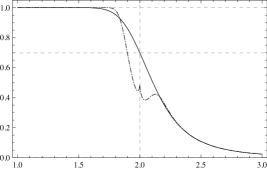
Comparing approximations (4.2) and (4.3) with (4.6), one can argue191919Using heuristic arguments and referring to exact formulas (2.2)–(2.4). that the results for proper and defective $\mathcal{I\hskip-0.5pt/I}$  sums in Example 2.1 must border seamlessly. But the normal (with $0<c<c^{\ast}=\mathsf{E}{Y}/\mathsf{E}{T}$) and quasi–normal (with $c>c^{\ast}$) approximations (4.2) and (4.3) do not border seamlessly. Moreover (see Fig. 3), both of them are either poor, or invalid202020Quasi–normal approximation (4.3) formally requires $c>c^{\ast}$. The existence of $\varkappa>0$ is possible only if the tail of $Y$ is exponentially decreasing. for $c$ at or near the critical value $c^{\ast}$.

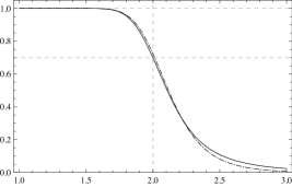
This distressing fact only indicates that the normal and quasi–normal approximations are deficient at $c^{\ast}$. In contrast, the inverse Gaussian approximation (see Fig. 4) does not have such a drawback. The case when $c$ is close to $c^{\ast}$ or even equals $c^{\ast}$ is routinely covered by the inverse Gaussian approximation.

Remark 4.5.

The intuitive explanation of deficiency of normal and quasi–normal approximations in the vicinity of the critical value $c^{\ast}$ is given in [64], Section 9.2.4. It is as follows. For exponentially distributed $X_{i}$ and $Y_{i}$, $i=1,2,\dots$, and $c$ equal to $c^{\ast}$ the compound sum is made up of the random variables with power moments of order no greater than $1/2$. Therefore, there is no reason to expect validity of normal and quasi–normal approximations.∎

The flaw of (4.2) and (4.3) in the vicinity od $c^{\ast}$ is merely a drawback of a particular mathematical technique. However, it has had a major negative impact on insurance modeling: while the insurance process in a close neighborhood of the critical point $c^{\ast}$ is of great importance (see details in [64]), it was overlooked for a long time partly due to this flaw. Moreover, the inverse Gaussian approximation allows (see [66]) to develop a new approach to risk measures different from value at risk (VaR).

5. Limit theorems for $\boldsymbol{\mathcal{R\hskip-0.5pt/D}}$ and proper $\boldsymbol{\mathcal{I\hskip-0.5pt/D}}$  sums

Kesten mentioned the part of modular analysis that deals with the lack of independence. It is best known because the area of “Markov chains, continuous time processes, and other situations in which the independence between summands no longer applies” is of particular interest. Among the tricks which reduce limit theorems for dependent summands to the case of independent summands, Kesten mentioned “Dœblin’s trick”.

Studying limit theorems for $\mathcal{R\hskip-0.5pt/D}$ and proper $\mathcal{I\hskip-0.5pt/D}$  sums, we will combine “Dœblin’s trick” and “Blackwell’s trick” and extend it to compound sums with general modular structure.

5.1. Compound sums with general modular structure

For $t>0$ and a complex basis $(T_{i},X_{i})$, $i=1,2,\dots$, we focus on unaltered complex compound sum ${S}_{N_{t}}$. We denote by $0<\mathcal{J}_{0}<\mathcal{J}_{1}<\dots$ a sequence of random indices, put

$$\begin{gathered}{\mathcal{\tau}}_{\hskip 1.0pt0}=\mathcal{J}_{0},\quad{\mathcal{T}}_{\hskip 1.0pt0}=\sum_{i=1}^{\mathcal{J}_{0}}\;T_{i},\quad{\mathcal{X}}_{\hskip 1.0pt0}=\sum_{i=1}^{\mathcal{J}_{0}}\;X_{i},\\[0.0pt] {\mathcal{\tau}}_{\hskip 1.0ptk}=\mathcal{J}_{k}-\mathcal{J}_{k-1},\quad{\mathcal{T}}_{\hskip 1.0ptk}=\sum_{i=\mathcal{J}_{k-1}+1}^{\mathcal{J}_{k}}T_{i},\quad{\mathcal{X}}_{\hskip 1.0ptk}=\sum_{i=\mathcal{J}_{k-1}+1}^{\mathcal{J}_{k}}X_{i},\end{gathered}$$

where $k=1,2,\dots$, and introduce the following definition.

Definition 5.1.

We say that the basis $(T_{i},X_{i})$, $i=1,2,\dots$, allows a modular structure if there exist a.s.  finite random indices $0<\mathcal{J}_{0}<\mathcal{J}_{1}<\dots$, such that

  • (i)

    the random vectors $({\mathcal{\tau}}_{\hskip 1.0ptk},{\mathcal{T}}_{\hskip 1.0ptk},{\mathcal{X}}_{\hskip 1.0ptk})$ are independent for $k=0,1,\dots$, and identically distributed for $k=1,2,\dots$,

  • (ii)

    ${V}_{\mathcal{J}_{k}}>\max_{0\leqslant i\leqslant\mathcal{J}_{k}-1}{V}_{i}$, $k=0,1,\dots$, i.e., $\mathcal{J}_{i}$, $i=0,1,\dots$, are upper record moments of the sequence ${V}_{n}=\sum_{i=1}^{n}T_{i}$, $n=1,2,\dots$.

For modular i.i.d.  random vectors $({\mathcal{X}}_{\hskip 1.0ptk},{\mathcal{T}}_{\hskip 1.0ptk},{\mathcal{\tau}}_{\hskip 1.0ptk})\overset{d}{=}({\mathcal{X}}_{\hskip 1.0pt},{\mathcal{T}}_{\hskip 1.0pt},{\mathcal{\tau}}_{\hskip 1.0pt})$, $k=1,2,\dots$, we use the shorthand notation $\mu_{{\mathcal{\tau}}_{\hskip 1.0pt}}=\mathsf{E}{\mathcal{\tau}}_{\hskip 1.0pt}$, $\mu_{{\mathcal{T}}_{\hskip 1.0pt}}=\mathsf{E}{\mathcal{T}}_{\hskip 1.0pt}$, $\mu_{{\mathcal{X}}_{\hskip 1.0pt}}=\mathsf{E}{\mathcal{X}}_{\hskip 1.0pt}$, $\sigma_{{\mathcal{\tau}}_{\hskip 1.0pt}}^{2}=\mathsf{D}{\mathcal{\tau}}_{\hskip 1.0pt}$, $\sigma_{{\mathcal{T}}_{\hskip 1.0pt}}^{2}=\mathsf{D}{\mathcal{T}}_{\hskip 1.0pt}$, $\sigma_{{\mathcal{X}}_{\hskip 1.0pt}}^{2}=\mathsf{D}{\mathcal{X}}_{\hskip 1.0pt}$. For $\hat{\mathcal{\tau}}^{\hskip 1.0pt}={\mathcal{\tau}}_{\hskip 1.0pt}-\mu_{{\mathcal{\tau}}_{\hskip 1.0pt}}$, $\hat{\mathcal{T}}^{\hskip 1.0pt}={\mathcal{T}}_{\hskip 1.0pt}-\mu_{{\mathcal{T}}_{\hskip 1.0pt}}$, $\hat{\mathcal{X}}^{\hskip 1.0pt}={\mathcal{X}}_{\hskip 1.0pt}-\mu_{{\mathcal{X}}_{\hskip 1.0pt}}$, and write $\varkappa_{{\mathcal{T}}_{\hskip 1.0pt}{\mathcal{\tau}}_{\hskip 1.0pt}}=\mathsf{E}\hat{\mathcal{T}}^{\hskip 1.0pt}\!\hat{\mathcal{\tau}}^{\hskip 1.0pt}$, $\varkappa_{{\mathcal{X}}_{\hskip 1.0pt}{\mathcal{T}}_{\hskip 1.0pt}}=\mathsf{E}\hat{\mathcal{X}}^{\hskip 1.0pt}\hat{\mathcal{T}}^{\hskip 1.0pt}$, $\varkappa_{{\mathcal{X}}_{\hskip 1.0pt}{\mathcal{\tau}}_{\hskip 1.0pt}}=\mathsf{E}\hat{\mathcal{X}}^{\hskip 1.0pt}\hat{\mathcal{\tau}}^{\hskip 1.0pt}$, $\rho_{{\mathcal{T}}_{\hskip 1.0pt}{\mathcal{\tau}}_{\hskip 1.0pt}}=\varkappa_{{\mathcal{T}}_{\hskip 1.0pt}{\mathcal{\tau}}_{\hskip 1.0pt}}/(\sigma_{{\mathcal{T}}_{\hskip 1.0pt}}\sigma_{{\mathcal{\tau}}_{\hskip 1.0pt}})$ $\rho_{{\mathcal{X}}_{\hskip 1.0pt}{\mathcal{T}}_{\hskip 1.0pt}}=\varkappa_{{\mathcal{X}}_{\hskip 1.0pt}{\mathcal{T}}_{\hskip 1.0pt}}/(\sigma_{{\mathcal{X}}_{\hskip 1.0pt}}\sigma_{{\mathcal{T}}_{\hskip 1.0pt}})$ $\rho_{{\mathcal{X}}_{\hskip 1.0pt}{\mathcal{\tau}}_{\hskip 1.0pt}}=\varkappa_{{\mathcal{X}}_{\hskip 1.0pt}{\mathcal{\tau}}_{\hskip 1.0pt}}/(\sigma_{{\mathcal{X}}_{\hskip 1.0pt}}\sigma_{{\mathcal{\tau}}_{\hskip 1.0pt}})$. We further introduce zero–mean block random variables212121Note that $\mathsf{E}\big{(}{\mathcal{R_{missing}}{}}_{\hskip 1.0pt\!{\mathcal{X}}_{\hskip 1.0pt}\!{\mathcal{T}}_{\hskip 1.0pt}}^{2}\big{)}$ is the same as $\mathsf{D}\big{(}{\mathcal{R_{missing}}{}}_{\hskip 1.0pt\!{\mathcal{X}}_{\hskip 1.0pt}\!{\mathcal{T}}_{\hskip 1.0pt}}\big{)}$ and $\mathsf{E}\big{(}{\mathcal{R_{missing}}{}}_{\hskip 1.0pt\!{\mathcal{\tau}}_{\hskip 1.0pt}\!{\mathcal{T}}_{\hskip 1.0pt}}^{2}\big{)}$ is the same as $\mathsf{D}\big{(}{\mathcal{R_{missing}}{}}_{\hskip 1.0pt\!{\mathcal{\tau}}_{\hskip 1.0pt}\!{\mathcal{T}}_{\hskip 1.0pt}}\big{)}$.

$\displaystyle{\mathcal{R_{missing}}{}}_{\hskip 1.0pt\!{\mathcal{T}}_{\hskip 1.0pt}{\mathcal{\tau}}_{\hskip 1.0pt}}$ $\displaystyle=\mu_{{\mathcal{T}}_{\hskip 1.0pt}}\,{\mathcal{\tau}}_{\hskip 1.0pt}-\mu_{{\mathcal{\tau}}_{\hskip 1.0pt}}{\mathcal{T}}_{\hskip 1.0pt}$ $\displaystyle{\mathcal{R_{missing}}{}}_{\hskip 1.0pt\!{\mathcal{X}}_{\hskip 1.0pt}\!{\mathcal{T}}_{\hskip 1.0pt}}=\mu_{{\mathcal{T}}_{\hskip 1.0pt}}{\mathcal{X}}_{\hskip 1.0pt}-\mu_{{\mathcal{X}}_{\hskip 1.0pt}}{\mathcal{T}}_{\hskip 1.0pt}$
   and
$\displaystyle=\mu_{{\mathcal{T}}_{\hskip 1.0pt}}\hat{\mathcal{\tau}}^{\hskip 1.0pt}-\mu_{{\mathcal{\tau}}_{\hskip 1.0pt}}\hat{\mathcal{T}}^{\hskip 1.0pt},$ $\displaystyle=\mu_{{\mathcal{T}}_{\hskip 1.0pt}}\hat{\mathcal{X}}^{\hskip 1.0pt}-\mu_{{\mathcal{X}}_{\hskip 1.0pt}}\hat{\mathcal{T}}^{\hskip 1.0pt}$

and put

$$\begin{gathered}\mathcal{M}_{N}{\,\!}=\mu_{{\mathcal{\tau}}_{\hskip 1.0pt}}\mu_{{\mathcal{T}}_{\hskip 1.0pt}}^{-1},\quad\mathcal{D}_{N}^{\,2}{\,}=\mathsf{E}\big{(}{\mathcal{R_{missing}}{}}_{\hskip 1.0pt\!{\mathcal{T}}_{\hskip 1.0pt}{\mathcal{\tau}}_{\hskip 1.0pt}}^{2}\big{)}\,\mu_{{\mathcal{T}}_{\hskip 1.0pt}}^{-3},\\[2.0pt] \mathcal{M}_{{S}}{\hskip 0.6pt\!}=\mu_{{\mathcal{X}}_{\hskip 1.0pt}}\mu_{{\mathcal{T}}_{\hskip 1.0pt}}^{-1},\quad\mathcal{D}_{{S}}^{\,2}{\,}=\mathsf{E}\big{(}{\mathcal{R_{missing}}{}}_{\hskip 1.0pt\!{\mathcal{X}}_{\hskip 1.0pt}\!{\mathcal{T}}_{\hskip 1.0pt}}^{2}\big{)}\mu_{{\mathcal{T}}_{\hskip 1.0pt}}^{-3},\\[0.0pt] \mathcal{B}_{{S}N}{\,\!}=\mathsf{E}\big{(}{\mathcal{R_{missing}}{}}_{\hskip 1.0pt\!{\mathcal{T}}_{\hskip 1.0pt}{\mathcal{\tau}}_{\hskip 1.0pt}}{\mathcal{R_{missing}}{}}_{\hskip 1.0pt\!{\mathcal{X}}_{\hskip 1.0pt}\!{\mathcal{T}}_{\hskip 1.0pt}}\big{)}\,\mu_{{\mathcal{T}}_{\hskip 1.0pt}}^{-3},\quad\mathcal{\rho}_{{S}\!N}{\,\!}=\mathcal{B}_{{S}N}{\,}\big{(}\mathcal{D}_{{S}}^{\,}{\,}\mathcal{D}_{N}^{\,}{\,\!}\big{)}^{-1}.\end{gathered}$$

Assumption (i) tackles “dependence complexity”, while (ii) takes hold of “irregularity complexity”, in both cases by reducing the original complex compound sum to a simple modular compound sum with simple modular basis $({\mathcal{T}}_{\hskip 1.0ptk},{\mathcal{X}}_{\hskip 1.0ptk})$, $k=1,2,\dots$. It consists of i.i.d.  modular random vectors with $s$–components positive. Moreover, if ${V}_{\mathcal{J}_{k}}<t$, then crossing level $t$ cannot occur inside $k$th block or inside blocks with a smaller index.

With $\mathsf{R}_{\,}(x,y)=\dfrac{x-\mathcal{\rho}_{{S}\!N}{\,\!}y}{1-\mathcal{\rho}_{{S}\!N}^{2}{\,}}$, we will use the following notation:

$$\mathcal{K}_{(3,0)}=\,\mathsf{E}\big{(}{\mathcal{R_{missing}}{}}_{\hskip 1.0pt\!{\mathcal{X}}_{\hskip 1.0pt}\!{\mathcal{T}}_{\hskip 1.0pt}}^{3}\big{)}\mu_{{\mathcal{T}}_{\hskip 1.0pt}}^{-4}\mathcal{D}_{{S}}^{\,-3}{\,}-3\mathsf{R}_{\,}({L}_{1},{L}_{2}),$$

where

$\displaystyle{L}_{1}=$ $\displaystyle\,\big{(}\varkappa_{{\mathcal{X}}_{\hskip 1.0pt}{\mathcal{\tau}}_{\hskip 1.0pt}}(\mu_{{\mathcal{\tau}}_{\hskip 1.0pt}}\sigma_{{\mathcal{T}}_{\hskip 1.0pt}}^{2}-\mu_{{\mathcal{T}}_{\hskip 1.0pt}}\varkappa_{{\mathcal{T}}_{\hskip 1.0pt}{\mathcal{\tau}}_{\hskip 1.0pt}})-\sigma_{{\mathcal{\tau}}_{\hskip 1.0pt}}^{2}(\mu_{{\mathcal{X}}_{\hskip 1.0pt}}\sigma_{{\mathcal{T}}_{\hskip 1.0pt}}^{2}-\mu_{{\mathcal{T}}_{\hskip 1.0pt}}\varkappa_{{\mathcal{X}}_{\hskip 1.0pt}{\mathcal{T}}_{\hskip 1.0pt}})$
$\displaystyle+\varkappa_{{\mathcal{T}}_{\hskip 1.0pt}{\mathcal{\tau}}_{\hskip 1.0pt}}(\mu_{{\mathcal{X}}_{\hskip 1.0pt}}\varkappa_{{\mathcal{T}}_{\hskip 1.0pt}{\mathcal{\tau}}_{\hskip 1.0pt}}-\mu_{{\mathcal{\tau}}_{\hskip 1.0pt}}\varkappa_{{\mathcal{X}}_{\hskip 1.0pt}{\mathcal{T}}_{\hskip 1.0pt}})\big{)}\mu_{{\mathcal{T}}_{\hskip 1.0pt}}^{-3}\mathcal{D}_{{S}}^{\,-1}{\,}\mathcal{D}_{N}^{\,-2}{\,},$
$\displaystyle{L}_{2}=$ $\displaystyle\,\big{(}-\varkappa_{{\mathcal{X}}_{\hskip 1.0pt}{\mathcal{\tau}}_{\hskip 1.0pt}}(\mu_{{\mathcal{X}}_{\hskip 1.0pt}}\sigma_{{\mathcal{T}}_{\hskip 1.0pt}}^{2}-\mu_{{\mathcal{T}}_{\hskip 1.0pt}}\varkappa_{{\mathcal{X}}_{\hskip 1.0pt}{\mathcal{T}}_{\hskip 1.0pt}})+\sigma_{{\mathcal{X}}_{\hskip 1.0pt}}^{2}(\mu_{{\mathcal{\tau}}_{\hskip 1.0pt}}\sigma_{{\mathcal{T}}_{\hskip 1.0pt}}^{2}-\mu_{{\mathcal{T}}_{\hskip 1.0pt}}\varkappa_{{\mathcal{T}}_{\hskip 1.0pt}{\mathcal{\tau}}_{\hskip 1.0pt}})$
$\displaystyle-\varkappa_{{\mathcal{X}}_{\hskip 1.0pt}{\mathcal{T}}_{\hskip 1.0pt}}(\mu_{{\mathcal{\tau}}_{\hskip 1.0pt}}\varkappa_{{\mathcal{X}}_{\hskip 1.0pt}{\mathcal{T}}_{\hskip 1.0pt}}-\mu_{{\mathcal{X}}_{\hskip 1.0pt}}\varkappa_{{\mathcal{T}}_{\hskip 1.0pt}{\mathcal{\tau}}_{\hskip 1.0pt}})\big{)}\mu_{{\mathcal{T}}_{\hskip 1.0pt}}^{-3}\mathcal{D}_{{S}}^{\,-2}{\,}\mathcal{D}_{N}^{\,-1}{\,}.$

It can be shown by direct algebra that $\mathsf{R}_{\,}\big{(}{L}_{1},{L}_{2}\big{)}=-\big{(}\mu_{{\mathcal{X}}_{\hskip 1.0pt}}\sigma_{{\mathcal{T}}_{\hskip 1.0pt}}^{2}-\mu_{{\mathcal{T}}_{\hskip 1.0pt}}\varkappa_{{\mathcal{X}}_{\hskip 1.0pt}{\mathcal{T}}_{\hskip 1.0pt}}\big{)}\,\mathcal{D}_{{S}}^{\,-1}{\,}\mu_{{\mathcal{T}}_{\hskip 1.0pt}}^{-2}$. Finally, we introduce

$\displaystyle\eta_{\hskip 1.0pt1}$ $\displaystyle=\mathsf{E}{\mathcal{X}}_{\hskip 1.0pt0}+\mu_{{\mathcal{T}}_{\hskip 1.0pt}}^{-1}\sum_{s=1}^{\infty}\int_{-\infty}^{\infty}x\int_{0}^{\infty}\mathsf{P}\big{\{}{\mathcal{\tau}}_{\hskip 1.0pt1}\geqslant s,{\mathcal{N}}_{\hskip 1.0pt}(t)=s,{\mathcal{X}}_{\hskip 1.0pt0}^{\hskip 1.0pt(s)}\in dx\big{\}}\,dt,$
$\displaystyle\eta_{\hskip 1.0pt2}$ $\displaystyle=\mathsf{E}{\mathcal{T}}_{\hskip 1.0pt0}+\mu_{{\mathcal{T}}_{\hskip 1.0pt}}^{-1}\sum_{s=1}^{\infty}\int_{0}^{\infty}t\,\mathsf{P}\big{\{}{\mathcal{\tau}}_{\hskip 1.0pt1}\geqslant s,{\mathcal{N}}_{\hskip 1.0pt}(t)=s\big{\}}\,dt,$
$\displaystyle\eta_{\hskip 1.0pt3}$ $\displaystyle=\mathsf{E}{\mathcal{\tau}}_{\hskip 1.0pt0}+\mu_{{\mathcal{T}}_{\hskip 1.0pt}}^{-1}\sum_{s=1}^{\infty}s\int_{0}^{\infty}\mathsf{P}\big{\{}{\mathcal{\tau}}_{\hskip 1.0pt1}\geqslant s,{\mathcal{N}}_{\hskip 1.0pt}(t)=s\big{\}}\,dt,$

where ${\mathcal{X}}_{\hskip 1.0pt0}^{\hskip 1.0pt(s)}=\sum_{k=\mathcal{J}_{0}+1}^{\mathcal{J}_{0}+s}X_{k}$ and ${\mathcal{N}}_{\hskip 1.0pt}(t)=\inf\big{\{}n\geqslant 1:\sum_{k=\mathcal{J}_{0}+1}^{\mathcal{J}_{0}+n}T_{k}>t\big{\}}$, or $\infty$, if the set is empty.

Theorem 5.1 below is formulated under the following conditions.

Condition $\boldsymbol{V}$ (Non–degenerate correlation matrix) $\mathsf{det}\,{{{Q}}}>0$ for the correlation matrix

$${{{Q}}}={Cor}\big{(}{\mathcal{X}}_{\hskip 1.0pt1},{\mathcal{T}}_{\hskip 1.0pt1},{\mathcal{\tau}}_{\hskip 1.0pt1}\big{)}=\left(\begin{matrix}1&\rho_{{\mathcal{X}}_{\hskip 1.0pt}{\mathcal{T}}_{\hskip 1.0pt}}&\rho_{{\mathcal{X}}_{\hskip 1.0pt}{\mathcal{\tau}}_{\hskip 1.0pt}}\\[0.0pt] \rho_{{\mathcal{X}}_{\hskip 1.0pt}{\mathcal{T}}_{\hskip 1.0pt}}&1&\rho_{{\mathcal{T}}_{\hskip 1.0pt}{\mathcal{\tau}}_{\hskip 1.0pt}}\\[0.0pt] \rho_{{\mathcal{X}}_{\hskip 1.0pt}{\mathcal{\tau}}_{\hskip 1.0pt}}&\rho_{{\mathcal{T}}_{\hskip 1.0pt}{\mathcal{\tau}}_{\hskip 1.0pt}}&1\end{matrix}\right).$$

Condition $\boldsymbol{P}_{\boldsymbol{}}$ (Bounded density condition) For an integer $n\geqslant 1$, there exists a bounded convolution power $f_{{\mathcal{T}}_{\hskip 1.0pt},{\mathcal{\tau}}_{\hskip 1.0pt}}^{*n}(x,n)$ w.r.t.  Lebesgue measure.

Condition $\boldsymbol{L}$ (Lattice condition) The integer–valued random variable ${\mathcal{\tau}}_{\hskip 1.0pt1}$ assumes values in the set of natural numbers with maximal span $1$.

Condition $\boldsymbol{C}$ (Uniform Cramér’s condition)

$$\overline{\lim}_{|t_{1}|\to\infty}\big{|}\,\mathsf{E}\exp\big{\{}it_{1}{\mathcal{X}}_{\hskip 1.0pt}+it_{2}{\mathcal{T}}_{\hskip 1.0pt}+it_{3}{\mathcal{\tau}}_{\hskip 1.0pt}\big{\}}\big{|}<1$$

for all $t_{2},t_{3}\in\mathsf{R}$.

Condition $\boldsymbol{B}_{\boldsymbol{(r,s)}}$ (Block moments condition) For $r,s>0$

  • (i)

    $\mathsf{E}\hskip 1.0pt\big{(}\mathcal{J}_{0}^{\hskip 1.0ptr}\big{)}<\infty$, $\mathsf{E}\big{(}{\mathcal{\tau}}_{\hskip 1.0pt1}^{s}\big{)}<\infty$,

  • (ii)

    $\mathsf{E}\bigg{(}\bigg{[}\displaystyle\sum_{k=1}^{\mathcal{J}_{0}}\big{|}\,T_{k}\big{|}\,\bigg{]}^{r}\bigg{)}<\infty$, $\mathsf{E}\bigg{(}\bigg{[}\displaystyle\sum_{k=\mathcal{J}_{0}+1}^{\mathcal{J}_{1}}\big{|}\,T_{k}\big{|}\,\bigg{]}^{\hskip-1.0pts}\bigg{)}<\infty$,

  • (iii)

    $\mathsf{E}\bigg{(}\bigg{[}\displaystyle\sum_{k=1}^{\mathcal{J}_{0}}\big{|}\,X_{k}\big{|}\,\bigg{]}^{r}\bigg{)}<\infty$, $\mathsf{E}\bigg{(}\bigg{[}\displaystyle\sum_{k=\mathcal{J}_{0}+1}^{\mathcal{J}_{1}}\big{|}\,X_{k}\big{|}\,\bigg{]}^{\hskip-1.0pts}\,\bigg{)}<\infty$.

The following theorem is Theorem 1 (III) in [62].

Theorem 5.1.

Assume that the basis $(T_{i},X_{i})$, $i=1,2,\dots$, of the complex compound sum ${S}_{N_{t}}$ allows a modular structure. If conditions ${V}$, ${P}$, ${L}$, ${C}$, and ${B}_{(k-\frac{3}{2},k)}$ with $k>3$ are satisfied, then there exist polynomials $\mathsf{Q}_{\,r}(x)$, $r=1,2,\dots,k-3$, of degree $3r-1$ such that

$\displaystyle\sup_{x\in\mathsf{R}}\,\bigg{|}\,\mathsf{P}\big{\{}{S}_{N_{t}}-\mathcal{M}_{{S}}{\hskip 0.6ptt}\leqslant x\mathcal{D}_{{S}}^{\,}{\,t^{1/2}}\big{\}}-\varPhi_{\left({0},{1}\right)}(x)$
$\displaystyle\hskip 90.0pt-\sum_{r=1}^{k-3}\frac{\mathsf{Q}_{\,r}(x)}{t^{r/2}}\,\varphi_{\left({0},{1}\right)}(x)\,\bigg{|}=O\big{(}t^{(k-2)/2}\big{)},\quad t\to\infty.$

In particular,

$$\mathsf{Q}_{\,1}(x)=-\frac{1}{6}\;\mathcal{K}_{(3,0)}\mathsf{H}_{2}(x)+\mathsf{R}_{\,}({L}_{1},{L}_{2})-\frac{\mu_{{\mathcal{T}}_{\hskip 1.0pt}}\eta_{\hskip 1.0pt1}-\mu_{{\mathcal{X}}_{\hskip 1.0pt}}\eta_{\hskip 1.0pt2}}{\mathcal{D}_{{S}}^{\,}{\,}\mu_{{\mathcal{T}}_{\hskip 1.0pt}}}.$$
Sketch of proof of Theorem 5.1.

The proof, similarly to the proof of Theorem 3.2, consists of steps A–F.

Step  A:  use of fundamental identity.  Similar to (3.5), we use the total probability rule. Writing

$$\begin{gathered}{\mathcal{X}}_{\hskip 1.0pt}^{[r]}=\sum_{i=1}^{r}X_{i},\ {\mathcal{T}}_{\hskip 1.0pt}^{[r]}=\sum_{i=1}^{r}T_{i},\ {\mathcal{X}}_{\hskip 1.0pt}^{(s)}=\sum_{i=\mathcal{J}_{m}+1}^{\mathcal{J}_{m}+s}X_{i},\ {\mathcal{T}}_{\hskip 1.0pt}^{(s)}=\sum_{i=\mathcal{J}_{m}+1}^{\mathcal{J}_{m}+s}T_{i}\end{gathered}$$

and ${\mathcal{N}}_{\hskip 1.0pt}(t)=\inf\big{\{}s\geqslant 1:{\mathcal{T}}_{\hskip 1.0pt}^{(s)}>t\big{\}}$, we have

$\displaystyle\mathsf{P}\big{\{}{S}_{N_{t}}\leqslant x\big{\}}=\,\sum_{n=1}^{\infty}\mathsf{P}\big{\{}{S}_{N_{t}}\leqslant x,N_{t}=n\big{\}},$

where the right–hand side is the sum of, first, the expression

$\displaystyle\sum_{n=1}^{\infty}\sum_{r}\iint_{\begin{subarray}{c}0\leqslant t_{1}\leqslant t\\[1.0pt] 0\leqslant x_{1}\leqslant x\end{subarray}}\mathsf{P}\Big{\{}{\mathcal{\tau}}_{\hskip 1.0pt0}=r,{\mathcal{T}}_{\hskip 1.0pt}^{[r]}\in dt_{1},{\mathcal{X}}_{\hskip 1.0pt}^{[r]}\in dx_{1}\Big{\}}$
$\displaystyle\hskip 30.0pt\times\mathsf{P}\Big{\{}{\mathcal{\tau}}_{\hskip 1.0pt1}\geqslant n-r,{\mathcal{N}}_{\hskip 1.0pt}(t-t_{1})=n-r,{\mathcal{X}}_{\hskip 1.0pt}^{(n-r)}\leqslant x-x_{1}\Big{\}},$

which corresponds to the absence of complete blocks, and, second, the expression

$\displaystyle\sum_{n=1}^{\infty}\sum_{r,s}\sum_{m=1}^{n-(r+s)}\idotsint_{\begin{subarray}{c}0\leqslant t_{1}+t_{2}\leqslant t\\[1.0pt] 0\leqslant x_{1}+x_{2}\leqslant x\end{subarray}}\mathsf{P}\bigg{\{}\sum_{i=1}^{m}{\mathcal{X}}_{\hskip 1.0pti}\leqslant x-\big{(}x_{1}+x_{2}\big{)},$ (5.1)
$\displaystyle\hskip 100.0pt\sum_{i=1}^{m}{\mathcal{\tau}}_{\hskip 1.0pti}=n-(s+r)\,\bigg{|}\,\sum_{i=1}^{m}{\mathcal{T}}_{\hskip 1.0pti}=t-(t_{1}+t_{2})\big{)}\bigg{\}}$
$\displaystyle\hskip 30.0pt\times f_{{\mathcal{T}}_{\hskip 1.0pt}}^{*m}\big{(}t-(t_{1}+t_{2})\big{)}\,\mathsf{P}\Big{\{}{\mathcal{\tau}}_{\hskip 1.0pt0}=r,{\mathcal{T}}_{\hskip 1.0pt}^{[r]}\in dt_{1},{\mathcal{X}}_{\hskip 1.0pt}^{[r]}\in dx_{1}\Big{\}}$
$\displaystyle\hskip 30.0pt\times\mathsf{P}\Big{\{}{\mathcal{\tau}}_{\hskip 1.0pt1}\geqslant s,{\mathcal{N}}_{\hskip 1.0pt}(t_{2})=s,{\mathcal{X}}_{\hskip 1.0pt}^{(s)}\in dx_{2}\Big{\}}\,dt_{2}.$

It is clear that for large $t$ only the expression (5.1) matters.

In words, in (5.1) the first incomplete block is made up by $r$ summands and the value $t$ cannot be exceeded all over this block because $t_{1}<t$; there are $m$ complete blocks, and exceeding the value $t$ still cannot happen, but it does occurs on the $s$th summand of the the $(m+1)$th complete block consisting of more than $s$ summands.

Steps  B and C  remain essentially the same as in the proof of Theorem 3.2.

Step  D:  application of refined CLT.  The integrand in (5.1) is ready for application of Edgeworth’s expansion in three–dimensional hybrid integro–local–local CLT with non–uniform remainder term. These theorems see in [31][33].

Steps  E and F  are technically much more complicated than in the proof of refined elementary renewal theorem (3.2) and Theorem 3.2 (they require a number of special identities), but use essentially the same analytical methods. ∎

Remark 5.1.

Theorem 3.2 is a corollary of Theorem 5.1. For $\mathcal{I\hskip-0.5pt/I}$  basis $(T_{i},X_{i})$, $i=1,2,\dots$, the modular structure is yielded by random indices $0\equiv\mathbb{\ell}_{0}<\mathbb{\ell}_{1}<\dots$ and, using Wald’s identities, $\mathcal{M}_{{S}}{\hskip 0.6pt}$ is transformed into $M_{{S}}{\,}$, and $\mathcal{K}_{(3,0)}$ is transformed into $K_{(3,0)}$.∎

5.2. Limit theorems for $\boldsymbol{\mathcal{R\hskip-0.5pt/D}}$  sums with Markov dependence

Markov renewal process (see, e.g., [24], [78]) is a homogeneous two–dimensional Markov chain $(\xi_{k},T_{k})$, $k=0,1,\dots$, which takes values in a general state space $(\mathit{E}\times\mathsf{R}^{+},\mathcal{E}\otimes\mathcal{R})$. Its transition functions are defined by a semi–Markov transition kernel. Markov renewal processes and their counterpart, semi–Markov processes, are among the most popular models of applied probability222222See, e.g., two bibliographies on semi–Markov processes [85] and [86]. The former consists of about 600 papers by some 300 authors and the later of almost a thousand papers by more than 800 authors..

In the same way as for renewal process, this model can be reformulated in terms of $\mathcal{R\hskip-0.5pt/D}$  basis $(T_{i},X_{i})$, $i=1,2,\dots$, and $\mathcal{R\hskip-0.5pt/D}$  sum with Markov dependence. Under certain regularity conditions, the sequence $0<\mathcal{J}_{0}<\mathcal{J}_{1}<\dots$ from Definition 5.1 is built in [7], [72]. Theorem analogous to Theorem 5.1 see in [60].

Remark 5.2 (Refined CLT for Markov chains).

In the special case $T_{i}\equiv 1$, the $\mathcal{R\hskip-0.5pt/D}$  sum with Markov dependence becomes the ordinary sum ${S}_{n}$ of random variables defined on the Markov chain $\{\xi_{i}\}_{i\geqslant 0}$.

Originally, “Dœblin’s trick” was applied to ${S}_{n}$ with discrete $\{\xi_{i}\}_{i\geqslant 0}$. Subsequently, it was repeatedly noted (see, e.g., [25] and [68]) that not the full countable space structure is often needed, but just the existence of one single “proper” point. The results then carry over with only notational changes to the countable case and, moreover, to (by means of the “splitting technique” and its counterparts, see [8], [72], [73], and [68]) irreducible recurrent general state space Markov chain $\{\xi_{i}\}_{i\geqslant 0}$ which satisfies strong minorization condition. Using modular advanced technique, for discrete (see [14]) and general state space Markov chains (see [15], [57], [59]) Berry–Esseen’s estimate, Edgeworth’s expansions, and asymptotic results for large deviations in CLT have been obtained.∎

5.3. Limit theorems for proper $\boldsymbol{\mathcal{I\hskip-0.5pt/D}}$  sums with Markov dependence

Markov additive process (see, e.g., [23], [78]) is a generalization of Markov renewal process with $(\xi_{k},T_{k})$, $k=0,1,\dots$, taking values in $(\mathit{E}\times\mathsf{R},\mathcal{E}\otimes\mathcal{R})$ rather than in $(\mathit{E}\times\mathsf{R}^{+},\mathcal{E}\otimes\mathcal{R})$. Under certain regularity conditions, for proper $\mathcal{I\hskip-0.5pt/D}$  sums with Markov dependence, the sequence $0<\mathcal{J}_{0}<\mathcal{J}_{1}<\dots$ from Definition 5.1 is built in [4] and [5]. Loosely speaking, these are the ladder points at which regeneration occurs.

6. Analysis of defective $\boldsymbol{\mathcal{I\hskip-0.5pt/D}}$  sums

For defective $\mathcal{I\hskip-0.5pt/D}$  sums, a deep analytical insight, such as in the case of defective $\mathcal{I\hskip-0.5pt/I}$  sums, is (see, e.g., [70], [74][77]) hardly possible. An alternative is computer–intensive analysis (see, e.g., [2], [50]).

Note that the papers devoted to defective $\mathcal{I\hskip-0.5pt/D}$  sums with Markov dependence are formulated as a study of the ruin probabilities for risk processes of Markovian type. This link with the ruin theory not only suggests rational examples of defective $\mathcal{I\hskip-0.5pt/D}$  sums, but also indicates areas in which they are of major interest.

7. A concluding remark

Due credits must be given to Dœblin (1915–1940), who (see [51], [52], [67]) put forth (see [26][29]) the major innovative ideas of coupling, decomposition and dissection232323The English translation of the title of [26] is “On two problems of Kolmogorov concerning countable Markov chains”, with reference to [48]. Therefore, Dœblin’s glory in this regard is partly shared with Kolmogorov. in Markov chains. The contributions of many scientists after him are mere a development of his seminal ideas. In this regard, compelling is the phrase from [40], that “our goal is to isolate the key ingredients in Dœblin’s proof and use them to derive ergodic theorems for much more general Markov processes on a typically uncountable state space”.

Having created a tool for sequential analysis, Anscombe (see [6]) rediscovered that part of “Dœblin’s trick” (as Kesten called it in [46]), or “Dœblin’s method” (as Kolmogorov called it in [49]), which is the use of Kolmogorov’s inequality for maximum of partial sums. Rényi (see [81], [82]), when he adapted Anscombe’s advance to compound sums ${S}_{N_{t}}$ with $N_{t}$ more general242424In Rényi’s sums (see Remark 2.1), $N_{t}$ is dependent on i.i.d.  summands and $N_{t}/\,t\overset{\scriptscriptstyle{\mathsf{P}}}{\rightarrow}\varrho$, $t\to\infty$, but is of a general form. than in (2.1), acknowledged (see [82]) that “K.L. Chung kindly called my attention to the fact that the main idea of the proof (the application of the inequality of Kolmogorov $\dots$) given in [81] is due to Dœblin (see [26]). It has been recently proved $\dots$ that the method in question can lead to the proof of the most general form of Anscombe’s theorem.” Just the way it is in the world of ideas.

References

  • [1]
  • [2] Albrecher, H., and Kantor, J. (2002) Simulation of ruin probabilities for risk processes of Markovian type, Monte Carlo Methods and Appl., 8, 111–127.
  • [3] Alsmeyer, G. (1988) Second–order approximations for certain stopped sums in extended renewal theory, Advances in Applied Probability, 20, 391–410.
  • [4] Alsmeyer, G. (2000) The ladder variables of a Markov random walk, Probability and Mathematical Statistics, 20, 1, 151–168.
  • [5] Alsmeyer, G. (2018) Ladder epochs and ladder chain of a Markov random walk with discrete driving chain, Advances in Applied Probability, 50, 31–46.
  • [6] Anscombe, F.J. (1952) Large–sample theory of sequential estimation, Proc. Cambridge Phil. Soc., 48, 600–607.
  • [7] Athreya, K.B., McDonald, D., and Ney, P. (1978) Limit theorems for semi–Markov processes and renewal theory for Markov chains, Ann. Probab., 6, 788–797.
  • [8] Athreya, K.B., and Ney, P. (1978) A new approach to the limit theory of recurrent Markov chains, Trans. Amer. Math. Soc., 245, 493–501.
  • [9] von Bahr, B. (1974) Ruin probabilities expressed in terms of ladder height distributions, Scandinavian Actuarial Journal, 57, 190–204.
  • [10] Baldwin, C.Y., and Clark, K.B. (2000) Design Rules. Vol. 1: The Power of Modularity. MIT Press, Cambridge, MA.
  • [11] Bhattacharya, R.N., and Ranga Rao, R. (1976) Normal Approximation and Asymptotic Expansions. John Wiley & Sons, New York.
  • [12] Bingham, N.H. (1989) The work of A.N. Kolmogorov on strong limit theorems, Theory Probab. Appl., 34, 1, 129–139.
  • [13] Blackwell, D. (1953) Extension of a renewal theorem, Pacific J. Math., 3, 315–320.
  • [14] Bolthausen, E. (1980) The Berry–Esseen theorem for functionals of discrete Markov chains, Z. Wahrscheinlichkeitstheorie Verw. Geb., B. 54, 59–73.
  • [15] Bolthausen, E. (1982) The Berry–Esseen theorem for strongly mixing Harris recurrent Markov chains, Z. Wahrscheinlichkeitstheorie Verw. Geb., B. 60, 283–289.
  • [16] Brooks, F.P. (1975) The Mythical Man–Month: Essays on Software Engineering. Addison–Wesley, Reading.
  • [17] Brown, M., and Solomon, H. (1975) A second–order approximation for the variance of a renewal reward process, Stochastic Processes and their Applications, 3, 301–314.
  • [18] Chibisov, D.M. (2016) Bernoulli’s law of large numbers and the strong law of large numbers, Theory Probab. Appl., 60, 318–319.
  • [19] Chow, Y.S., and Teicher, H. (1997) Probability Theory. Independence, Interchangeability, Martingales. Springer Texts in Statistics, 3rd ed., Springer, New York.
  • [20] Chung, K.L. (1967) Markov Chains with Stationary Transition Probabilities. Springer, Berlin, Heidelberg, New York.
  • [21] Cox, D.R. (1970) Renewal Theory. Methuen & Co., London.
  • [22] Cox, D.R., and Miller, H.D. (2001) The Theory of Stochastic Processes. Chapman and Hall/CRC, Boca Raton.
  • [23] Çinlar, E. (1972) Markov additive processes. I, II, Probability Theory and Related Fields, 24, 85–93, 95–121.
  • [24] Çinlar, E. (1975) Markov renewal theory: a survey, Management Science, 21, 727–752.
  • [25] Dacunha–Castelle, D., and Duflo, M. (1986) Probability and Statistics. Vol. II. Springer, New York, Berlin, etc.
  • [26] Dœblin, W. (1938) Sur deux problèmes de M. Kolmogoroff concernant les chaînes dénombrables, Bull. Soc. Math. de France, 66, 210–220.
  • [27] Dœblin, W. (1938) Exposé de la théorie des chaînes simples constants de Markoff à un nombre fini d’états, Revue Math. de l’Union Interbalkanique, 2, 77–105.
  • [28] Dœblin, W. (1940) Éléments d’une théorie générale des chaînes simple constantes de Markoff, Ann. Sci. École Norm. Sup., 57, 61–111.
  • [29] Dœblin, W., and Fortet, R. (1937) Sur des chaînes à liaisons complètes, Bull. Soc. Math. de France, 65, 132–148.
  • [30] Doob, J.L. (1948) Renewal theory from the point of view of the theory of probability, Trans. Amer. Math. Soc., 63, 422–438.
  • [31] Dubinskaite, J. (1982) Limit theorems in $\mathsf{R}^{k}$. I, Lith. Math. J., 22, 129–140.
  • [32] Dubinskaite, J. (1984) Limit theorems in $\mathsf{R}^{k}$. II, Lith. Math. J., 24, 256–265.
  • [33] Dubinskaite, J. (1984) Limit theorems in $\mathsf{R}^{k}$. III, Lith. Math. J., 24, 352–334.
  • [34] Feller, W. (1940) On the integro–differential equations of purely discontinuous Markov processes, Trans. Amer. Math. Soc., 48, 488–515.
  • [35] Feller, W. (1941) On the integral equation of renewal theory, Ann. Math. Stat., 12, 243–267.
  • [36] Feller, W. (1949) Fluctuation theory of recurrent events, Trans. Amer. Math. Soc., 67, 98–119.
  • [37] Feller, W. (1971) An Introduction to Probability Theory and its Applications. Vol. II. 2nd ed., John Wiley & Sons, New York, etc.
  • [38] Gnedenko, B.V., and Korolev, V.Yu. (1996) Random Summation. Limit Theorems and Applications. CRC Press: Boca Raton.
  • [39] Gœtze, F., and Hipp, C. (1983) Asymptotic expansions for sums of weakly dependent random variables, Z. Wahrscheinlichkeitstheorie Verw. Geb., 64, 211–239.
  • [40] Griffeath, D. (1978) Coupling methods for Markov processes. Thesis, Cornell Univ. In: Rota, G.–C. (ed.) Studies in Probability and Ergodic Theory. Advances in Mathematics: Supplementary Studies, Vol. 2, 1–43. Academic Press, New York, etc.
  • [41] Gut, A. (2009) Stopped Random Walks. Limit Theorems and Applications. 2nd ed., Springer–Verlag, New York.
  • [42] Hervé, L., and Pène, F. (2010) The Nagaev–Guivarc’h method via the Keller–Liverani theorem, Bull. Soc. Math. de France, 138, 3, 415–489.
  • [43] Hipp, C. (1985) Asymptotic expansions in the central limit theorem for compound and Markov processes, Z. Wahrscheinlichkeitstheorie Verw. Geb., 69, 361–385.
  • [44] Jewell, W.B. (1967) Fluctuations of a renewal–reward process, J. Math. Anal. Appl., 19, 2, 309–329.
  • [45] Karlin, S., and Taylor, H.M. (1975) A First Course in Stochastic Processes. 2nd ed., Academic Press, New York, etc.
  • [46] Kesten, H. (1977) Book review (of [80]), Bull. Amer. Math. Soc., 83, 696–697.
  • [47] Kingman, J.F.C. (1972) Regenerative phenomena. John Wiley & Sons, London, etc.
  • [48] Kolmogorov, A.N. (1936) Anfangsgründe der Theorie der Markoffschen Ketten mit unendlich vielen möglichen Zuständen, Mat. Sbornik, N. Ser., 1, 607–610.
  • [49] Kolmogorov, A.N. (1949) A local limit theorem for classical Markov chains, Izv. Akad. Nauk SSSR, Ser. Mat. 13, 281–300 (in Russian).
  • [50] Lehtonen, T., and Nyrhinen, H. (1992) On asymptotically efficient simulation of ruin probabilities in a Markovian environment, Scandinavian Actuarial Journal, 60–75.
  • [51] Lévy, P. (1955) W. Dœblin (V. Doblin) (1915–1940), Rev. Histoire Sci. Appl., 8, 107–115.
  • [52] Lindvall, T. (1991) W. Dœblin, 1915–1940, Ann. Probab., 19, 929–934.
  • [53] Loève, M. (1950) Fundamental limit theorems of probability theory, Ann. Math. Stat., 21, 321–338.
  • [54] Lotka, A. (1939) A contribution to the theory of self–renewing aggregates, with special reference to industrial replacement, Ann. Math. Stat., 10, 1–25.
  • [55] Malinovskii, V.K. (1984) On asymptotic expansions in the central limit theorem for Harris recurrent Markov chains, Soviet Math. Dokl., 29, 679–684.
  • [56] Malinovskii, V.K. (1985) On some asymptotic relations and identities for Harris recurrent Markov chains. In: Statistics and Control of Stochastic Processes, Optimization Software, 317–336.
  • [57] Malinovskii, V.K. (1987) Limit theorems for Harris Markov chains. I, Theory Probab. Appl., 31, 269–285.
  • [58] Malinovskii, V.K. (1988) On a limit theorem for dependent random variables, Ann. Academiæ Scientiarum Fennicæ, 13, 225–229.
  • [59] Malinovskii, V.K. (1990) Limit theorems for Harris Markov chains. II, Theory Probab. Appl., 34, 252–265.
  • [60] Malinovskii, V.K. (1991) On integral and local limit theorems for recursive252525Erroneous translation into English. In the original paper published in 1988 in Russian: “recurrent”. Markov renewal processes, Journal of Soviet Math., 57, 4, 3286–3301. [MR 91m: 60161] Translated from: Problems of Stability of Stoch. Models (1988), Ed. V.M. Zolotarev, VNIISI, Moscow, 100–115 (in Russian).
  • [61] Malinovskii, V.K. (1992) Asymptotic expansions in the central limit theorem for stopped random walks, Theory Probab. Appl., 36, 827–829.
  • [62] Malinovskii, V.K. (1994) Limit theorems for stopped random sequences I. Rates of convergence and asymptotic expansions, Theory Probab. Appl., 38, 673–693.
  • [63] Malinovskii, V.K. (1994) Corrected normal approximation for the probability of ruin within finite time, Scandinavian Actuarial Journal, 161–174.
  • [64] Malinovskii, V.K. (2021) Insurance Planning Models. World Scientific, Singapore.
  • [65] Malinovskii, V.K. (2021) Level–Crossing Problems and Inverse Gaussian Distributions. Chapman and Hall/CRC, Boca Raton.
  • [66] Malinovskii, V.K. (2021) Risk Measures and Insurance Solvency Benchmarks. Chapman and Hall/CRC, Boca Raton.
  • [67] Meyn, S.P., and Tweedie, R.L. (1993) The Dœblin decomposition, Contemporary Mathematics, 149, 211–225.
  • [68] Meyn, S.P., and Tweedie, R.L. (2009) Markov Chains and Stochastic Stability. 2nd ed., Cambridge Univ. Press, Cambridge, etc.
  • [69] Mikes, G. (1970) How to Be an Alien: A Handbook for Beginners and Advanced Pupils. Gardners Books.
  • [70] Mikosch, T., and Samorodnitsky, G. (2000) Ruin probability with claims modeled by a stationary ergodic stable process, Ann. Probab., 28, 1814–1851.
  • [71] Nummelin, E. (1978) A splitting technique for Harris recurrent chains, Z. Wahrscheinlichkeitstheorie Verw. Geb., 43, 309–318.
  • [72] Nummelin, E. (1978) Uniform and ratio limit theorems for Markov renewal and semi–regenerative processes on a general state space, Ann. Inst. H. Poincare, Sect. B, Vol. XIV, 119–143.
  • [73] Nummelin, E. (1984) General Irreducible Markov Chains and Non–negative Operators. Cambridge Univ. Press, Cambridge, etc.
  • [74] Nyrhinen, H. (1998) Rough descriptions of ruin for a general class of surplus processes, Advances in Applied Probability, 30, 1008–1026.
  • [75] Nyrhinen, H. (1999) Large deviations for the time of ruin, Journal of Applied Probability, 36, 733–746.
  • [76] Nyrhinen, H. (1999) On the ruin probabilities in a general economic environment, Stochastic Processes and their Applications, 83, 319–330.
  • [77] Nyrhinen, H. (2001) Finite and infinite time ruin probabilities in a stochastic economic environment, Stochastic Processes and their Applications, 92, 265–285.
  • [78] Pacheco, A., Prabhu, N.U., and Tang, L.C. (2009) Markov–modulated Processes and Semiregenerative Phenomena. World Scientific, New Jersey, etc.
  • [79] Parnas, D.L. (1972) On the criteria to be used in decomposing systems into modules, Communications of the Association for Computing Machinery (ACM), 15, 1053–1058.
  • [80] Petrov, V.V. (1975) Sums of Independent Random Variables. Springer, Berlin, etc.
  • [81] Rényi, A. (1957) On the asymptotic distribution of the sum of a random number of independent random variables, Acta Math. Acad. Sci. Hungar., 8, 193–199.
  • [82] Rényi, A. (1960) On the central limit theorem for the sum of a random number of independent random variables, Acta Math. Acad. Sci. Hungar., 11, 97–102.
  • [83] Rio, E. (2017) Asymptotic Theory of Weakly Dependent Random Processes. Springer, New York.
  • [84] Robbins, H. (1948) The asymptotic distribution of the sum of a random number of random variables, Bull. Amer. Math. Soc., 54, 1151–1161.
  • [85] Teugels, J.L. (1976) A bibliography on semi–Markov processes, Journal of Computational and Applied Mathematics, 2, 125–144.
  • [86] Teugels, J.L. (1986) A second bibliography on semi–Markov processes, In: Semi–Markov Models. Theory and Applications, ed. J. Janssen, 507–584, Plenum Press, New York.
  • [87] Tikhomirov, A.N. (1981) On the convergence rate in the central limit theorem for weakly dependent random variables, Theory Probab. Appl., 25, 790–809.
  • [88] Wolff, R.W. (1989) Stochastic Modeling and the Theory of Queues. Prentice–Hall.