Cosmology-independent Photon Mass Limits from Localized Fast Radio Bursts by using Artificial Neural Networks
Abstract
A hypothetical photon mass, , can produce a frequency-dependent vacuum dispersion of light, which leads to an additional time delay between photons with different frequencies when they propagate through a fixed distance. The dispersion measure–redshift measurements of fast radio bursts (FRBs) have been widely used to constrain the rest mass of the photon. However, all current studies analyzed the effect of the frequency-dependent dispersion for massive photons in the standard CDM cosmological context. In order to alleviate the circularity problem induced by the presumption of a specific cosmological model based on the fundamental postulate of the masslessness of photons, here we employ a new model-independent smoothing technique, Artificial Neural Network (ANN), to reconstruct the Hubble parameter function from 34 cosmic-chronometer measurements. By combining observations of 32 well-localized FRBs and the function reconstructed by ANN, we obtain an upper limit of , or equivalently (, or equivalently ) at the () confidence level. This is the first cosmology-independent photon mass limit derived from extragalactic sources.
pacs:
14.70.Bh, 41.20.Jb, 52.25.Os, 95.85.BhI Introduction
As a fundamental postulate of Maxwell’s electromagnetism and Einstein’s special relativity, the principle of the constancy of the speed of light implies the masslessness of photons, as elucidated by the particle-wave duality. This principle is also embraced within the framework of general relativity (GR). However, even a very minute photon mass, if existent, would necessitate new physical theories, such as the renowned de Broglie-Proca theory (De Broglie, 1922; Proca, 1936), the model of massive photons as an explanation for dark energy (Kouwn et al., 2016), and other new ideas in the standard-model extension with massive photons (Spallicci et al., 2021). Consequently, achieving precise constraints on the rest mass of photon, denoted as , remains an imperative.
Numerous experimental and observational constraints on have been derived from various effects resulting from the hypothetical nonzero photon mass. These include tests of Coulomb’s inverse square law (Williams et al., 1971), the Cavendish torsion balance (Lakes, 1998; Luo et al., 2003), gravitational deflection of electromagnetic waves (Lowenthal, 1973), mechanical stability of magnetized gas in galaxies (Chibisov, 1976), magneto-hydrodynamic phenomena of the solar wind (Ryutov, 1997, 2007; Liu and Shao, 2012; Retinò et al., 2016), Jupiter’s magnetic field (Davis et al., 1975), the spindown of a pulsar (Yang and Zhang, 2017), among others. However, these constraints are contingent upon specific theories of massive photons and are thus dynamic tests in nature.
In contrast, a kinematic test based on the dispersion effect of the speed of light in vacuum is more inherently pure (Tu et al., 2005a, b). The dispersion relation for massive photons is governed by
| (1) |
where represents the momentum. The group velocity of a photon with energy can be expressed as
| (2) |
where is the Planck constant and the last term is valid when . Eq. (2) suggests that if two photons with different frequencies are emitted simultaneously from the same source, they will be observed at different times due to their different velocities. Fast radio bursts (FRBs) provide an excellent celestial laboratory for detecting this dispersion effect, owing to their characteristics of (i) short time durations, (ii) long propagation distances, and (iii) low-frequency emissions.
Based on the vacuum dispersion method, several studies have used FRBs to put stringent upper limits on the photon mass (Wu et al., 2016; Bonetti et al., 2016, 2017; Shao and Zhang, 2017; Xing et al., 2019; Wei and Wu, 2020; Wang et al., 2021; Chang et al., 2023; Lin et al., 2023; Wang et al., 2023, 2024). Since FRBs originate at cosmological distances, the cosmic expansion rate has to be considered in constraining the photon mass . In all previous studies, the required information is calculated within the standard CDM cosmological model. It should, however, be emphasized that CDM is rooted in the framework of GR, which also embraces the postulate of the constancy of light speed. Thus, there is a circularity problem in constraining the photon mass. To address this problem, one has to determine the Hubble parameter in a cosmology-independent way.
In this work, we propose a novel nonparametric approach, utilizing the Artificial Neural Network (ANN) technology, to reconstruct a smooth function that best approximates the discrete measurements. By combining observations of well-localized FRBs and the function reconstructed by ANN, we aim to establish a cosmology-independent constraint on the rest mass of the photon. The paper is structured as follows. Section II introduces the theoretical framework and the observational data utilized for constraining the photon mass. Section III presents the cosmology-independent constraints on the photon mass and other relevant parameters. Finally, a brief summary and discussions are given in Section IV.
II Analysis Method and Data
II.1 Theoretical framework
In our analysis, the observed time delay between different frequencies for FRBs is attributed to two main factors: (i) the propagation of photons through the plasma distributed between the source of the FRB and the observer, and (ii) the non-zero rest mass of the photon.
-
•
Due to the interaction between the plasma and electromagnetic waves, photons with higher frequency travel faster than those with lower frequency , resulting in a dispersion effect. The time delay between photons of different frequencies caused by this dispersion effect can be described as (Lorimer and Kramer, 2012; Bentum et al., 2017)
(3) where is the plasma frequency with the number density of electrons , the charge of an electron , the mass of an electron , and the permittivity of vacuum . Here is the dispersion measure (DM) contributed by the plasma, which is defined as the integral of the number density of electrons along the line of propagation, given by .
For an extragalactic source, can be primarily divided into four components: the contributions from the Milky Way’s interstellar medium (), the Galactic halo (), the intergalactic medium (IGM; ), and the host galaxy (). Therefore, is given by
(4) where the factor converts the DM component of the host galaxy in the rest frame, denoted as , to the observed value .
-
•
According to Eq. (2), the time delay between massive photons of high and low frequencies can be expressed as:
(5) where is a newly defined function related to redshift,
(6) where is the Hubble parameter at redshift . Note that here differs from the dimensionless redshift function that defined in previous works, and it is in units of .
In our analysis, the total observed time delay is
| (7) |
Observationally, the time delay of all FRBs exhibits a frequency dependence of , while both and follow a behavior. Hence, it is natural for us to analogously define the equivalent DM arising from the massive photons as (Shao and Zhang, 2017)
| (8) |
Thus, the observed DM obtained from fitting the behavior in the total frequency-dependent time delay, can be written as:
| (9) |
Once we are able to properly estimate the value of each DM term in Eq. (4), can then be effectively extracted from , thereby providing an upper limit on the photon mass .
The term arising from the ionizing medium around our galaxy is well modeled by some galactic electron distribution models. Here we adopt the NE2001 model (Cordes and Lazio, 2002) for its wide application. The value of is challenging to estimate accurately, but it has been expected to lie within the range of (Prochaska and Zheng, 2019; Keating and Pen, 2020). Here, we conservatively adopt a Gaussian prior of (Wu et al., 2022; Wang et al., 2023).
The DM due to the IGM, , depends on the cosmological model and is largely influenced by the number of halos intersected along the propagation path. Due to density perturbations on large-scale structures, it is challenging to calculate the precise value of for individual FRBs. Instead, we typically calculate the average value of using (Deng and Zhang, 2014)
| (10) |
where is the baryon density parameter at the present day, is the Hubble constant, is the fraction of baryon in the IGM (Fukugita et al., 1998), is the gravitational constant, and is the mass of proton. The redshift-dependent function (in units of ) is defined by
| (11) |
However, the actual value of may deviate from the average due to the inhomogeneity of IGM. To account for this variability, we employ a one-parameter model to simulate the probability distribution of (Miralda-Escudé et al., 2000; Macquart et al., 2020; Wang et al., 2021), which is given by
| (12) |
where , is a normalization constant to ensure the integral of to be unity, is chosen to satisfy , and (Macquart et al., 2020). The fractional standard deviation of is approximated as , where is the free parameter that quantifies the strength of baryon feedback (Macquart et al., 2020). Both semi-analytic models and numerical simulations of the IGM and galaxy halos showed that the probability distribution of can be well fitted by the quasi-Gaussian form (i.e., Eq. 12) (McQuinn, 2014; Macquart et al., 2020). Therefore, this analytic form is adopted in our analysis.
The term is contributed by the source environment and the interstellar medium of the host galaxy, implying that the value of may vary significantly across different sources. To model this variability, we adopt a log-normal distribution for the probability density function of with the expression as (Macquart et al., 2020)
| (13) | ||||
where and are free parameters which are used to estimate the mean and standard deviation of , respectively.
With the analyses stated above, we formulate the joint likelihood function for a sample of localized FRBs as
| (14) |
where is the number of FRBs and denotes the likelihood for the -th FRB with the corrected observable DM as
| (15) | ||||
For a certain FRB at the redshift of , we can estimate the probability distribution of with the combination of Eqs. (12), (13), and (15), which gives the expression as
| (16) | ||||
Note that by Eq. (8), is a constant at a given . Denoting , , and as the probability density functions of random variables , , and , respectively. The equality holds for every non-negative independent random variables , , and , such that . As and are non-negative independent random variables, by setting , , and , it is easy to derive Eq. (16).
By maximizing the likelihood function , we can place constraints on the parameters in our model, including the rest mass of the photon . Nevertheless, there are two redshift-dependent functions, and (see Eqs. 6 and 11), to be determined. In previous works (Wu et al., 2016; Bonetti et al., 2016, 2017; Shao and Zhang, 2017; Xing et al., 2019; Wei and Wu, 2020; Wang et al., 2021; Chang et al., 2023; Lin et al., 2023; Wang et al., 2023), the conventional approach is to adopt the flat CDM cosmological model and replace the denominator with . Subsequently, and are calculated by treating the cosmological parameters and as fixed values. However, it is crucial to note that the CDM model is established within the framework of Einstein’s theory of GR, which is derived from one of the fundamental postulates–the masslessness of photons. Consequently, adopting this model introduces a logical circularity problem in constraining the rest mass of the photon. To circumvent this issue, it is necessary to employ a cosmology-independent method to describe the relation between the Hubble parameter and redshift .
II.2 Artificial Neural Network
Gaussian Process (GP) is a widely-used approach for studying cosmology in a model-independent manner. This method assumes that the reconstructed value at a given point follows a Gaussian distribution, and the relationship between function values at different points is characterized by a selected covariance function (Seikel et al., 2012). Besides, the reconstructed function of from GP tends to underestimate errors and is significantly influenced by the prior of the Hubble constant (Wei and Wu, 2017; Wang et al., 2017). In contrast, ANN, inspired by biological neural networks, is a mathematical model primarily used to discover intricate relationships between input and output data. The reconstructed function based on ANN makes no assumptions about the observational data and is entirely data-driven without parameterization of the function. Recently, Ref. Wang et al. (2020) developed a public code called ReFANN111https://github.com/Guo-Jian-Wang/refann for reconstructing functions from data using ANN. Their reconstructed function showed no sensitivity to the setting of , indicating that reconstructing from observational data using ANN may be more reliable than using GP. To make a cosmology-independent determination of , in this work we will reconstruct a smooth curve of from 34 model-independent measurements of using ReFANN.
The first step in using ReFANN to reconstruct a function from data is to find the best parameter configuration for the model used to train the data. Following the approach of Ref. Wang et al. (2020), we determine the optimal network model by minimizing the risk (Wasserman et al., 2001):
| (17) | ||||
where is the number of sample and is the fiducial value of at redshift . For our purposes, we only consider the number of hidden layers and neurons in the hidden layer. Through experimentation, we determined that the optimal model configuration involves a single hidden layer with 4096 neurons. Additionally, to reduce sensitivity to initialization and stabilize the distribution among variables, we employ batch normalization (Ioffe and Szegedy, 2015) in our network model, with the batch size set to half of the number of data points. We also use the Exponential Linear Unit (Clevert et al., 2015) as the activation function, with the hyperparameter set to be 1. Furthermore, we utilize the Adam optimizer (Kingma and Ba, 2014) to update the network parameters in each iteration of the training process.
Subsequently, we train this optimal network model with the observational data. This training process provides us with a predicted value of and its associated error at a given redshift . This predicted function represents an approximate reconstruction of based on the ANN model trained with observational data.
| Refs. | |||
| () | () | ||
| 0.09 | 69 | 12 | Jimenez et al. (2003) |
| 0.17 | 83 | 8 | Simon et al. (2005) |
| 0.27 | 77 | 14 | |
| 0.4 | 95 | 17 | |
| 0.9 | 117 | 23 | |
| 1.3 | 168 | 17 | |
| 1.43 | 177 | 18 | |
| 1.53 | 140 | 14 | |
| 1.75 | 202 | 40 | |
| 0.48 | 97 | 62 | Stern et al. (2010) |
| 0.88 | 90 | 40 | |
| 0.1791 | 75 | 4 | Moresco et al. (2012) |
| 0.1993 | 75 | 5 | |
| 0.3519 | 83 | 14 | |
| 0.5929 | 104 | 13 | |
| 0.6797 | 92 | 8 | |
| 0.7812 | 105 | 12 | |
| 0.8754 | 125 | 17 | |
| 1.037 | 154 | 20 | |
| 0.07 | 69 | 19.6 | Zhang et al. (2014) |
| 0.12 | 68.2 | 26.2 | |
| 0.2 | 72.9 | 29.6 | |
| 0.28 | 88.8 | 36.6 | |
| 1.363 | 160 | 33.6 | Moresco (2015) |
| 1.965 | 186.5 | 50.4 | |
| 0.3802 | 83 | 13.5 | Moresco et al. (2016) |
| 0.4004 | 77 | 10.2 | |
| 0.4247 | 87.1 | 11.2 | |
| 0.4497 | 92.8 | 12.9 | |
| 0.4783 | 80.9 | 9 | |
| 0.47 | 89 | 49.6 | Ratsimbazafy et al. (2017) |
| 0.75 | 98.8 | 33.6 | Borghi et al. (2022) |
| 0.8 | 113.1 | 25.22 | Jiao et al. (2023) |
| 1.26 | 135 | 65 | Tomasetti et al. (2023) |
II.3 Hubble parameter Data
The Hubble parameter , which quantifies the expansion rate of the universe as a function of time (or equivalently redshift), has been extensively used for exploring the nature of dark energy and testing modified theories of gravity. can be measured using two main methods. One approach is based on the detection of the radial baryon acoustic oscillation features (Gaztañaga et al., 2009; Blake et al., 2012; Samushia et al., 2013). However, this method relies on assumptions about the underlying cosmological model, typically the CDM model. Therefore, in our analysis, we focus exclusively on measurements obtained using another method, namely the cosmic chronometers (CC) method (Jimenez and Loeb, 2002). This method is model-independent as it relies on minimal assumptions, primarily the use of a Friedmann-Lemaître-Robertson-Walker metric. In this method, by combining the definition of and the relation between the scale factor and redshift, , can be rewritten as
| (18) |
This means that one can achieve a model-independent determination of by calculating the differential age of the universe using passively evolving galaxies at various redshifts. We compile the latest 34 CC measurements in Table 1, covering the redshift range of .
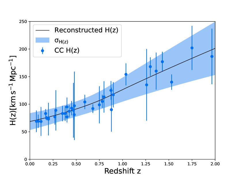
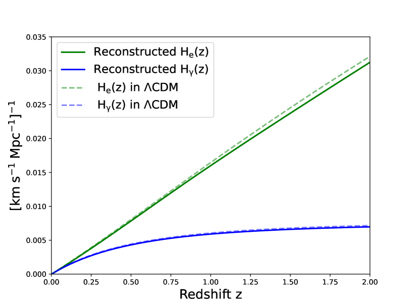
Having obtained the dataset of , we adopt ANN to reconstruct the function within the redshift range of , and the results are shown in Fig. 1. The black line represents the best fit, and the blue shaded area indicates the 1 confidence region of the reconstructed function. The redshift-dependent and functions can then be derived by integrating the reconstructed function with respect to redshift. As shown in Fig. 2, the reconstructed and functions exhibit significant differences in behavior as a function of redshift . Such distinctions are crucial for breaking parameter degeneracy and enhancing sensitivity in testing the photon mass when a few redshift measurements of FRBs are available (Bonetti et al., 2016, 2017; Shao and Zhang, 2017; Wei and Wu, 2020; Bentum et al., 2017). For comparison, we also plot and functions within the framework of the flat CDM model using Planck 2018 parameters ( and ) (Planck Collaboration et al., 2020). The corresponding theoretical curves are presented in Fig. 2 as dashed lines. It is evident that the reconstructions of and are roughly consistent with the predictions of the standard CDM model, implying that the ANN method can offer a reliable reconstructed function from the observational data.
II.4 Fast Radio Burst Data
Expanding upon the sample of 23 localized FRBs utilized in Ref. Wang et al. (2023), we incorporate 9 new localized FRBs recently detected by the 110-antenna Deep Synoptic Array Law et al. (2023). Note that another two new FRBs with redshift measurements, FRB 20220319D and FRB 20220914A, are not included in our sample. FRB 20220319D exhibits an observed value of , while the value calculated using the NE2001 model stands at , leading to its exclusion from our analysis. Furthermore, FRB 20220914A is omitted due to its notable deviation from the expected – relation outlined in Eq. (10). The total 32 localized FRBs, including their respective redshifts, , and , are provided in Table 2.
| Name | Refs. | |||
| FRB 20121102 | 0.19273 | 557 | 188.0 | Chatterjee et al. (2017) |
| FRB 20180301 | 0.3304 | 536 | 152.0 | Bhandari et al. (2022) |
| FRB 20180916 | 0.0337 | 348.76 | 200.0 | Marcote et al. (2020) |
| FRB 20180924 | 0.3214 | 361.42 | 40.5 | Bannister et al. (2019) |
| FRB 20181112 | 0.4755 | 589.27 | 102.0 | Prochaska et al. (2019) |
| FRB 20190102 | 0.291 | 363.6 | 57.3 | Bhandari et al. (2020) |
| FRB 20190523 | 0.66 | 760.8 | 37.0 | Ravi et al. (2019) |
| FRB 20190608 | 0.1178 | 338.7 | 37.2 | Chittidi et al. (2021) |
| FRB 20190611 | 0.378 | 321.4 | 57.83 | Heintz et al. (2020) |
| FRB 20190614 | 0.6 | 959.2 | 83.5 | Law et al. (2020) |
| FRB 20190711 | 0.522 | 593.1 | 56.4 | Heintz et al. (2020) |
| FRB 20190714 | 0.2365 | 504 | 38.0 | Heintz et al. (2020) |
| FRB 20191001 | 0.234 | 506.92 | 44.7 | Heintz et al. (2020) |
| FRB 20191228 | 0.2432 | 297.5 | 33.0 | Bhandari et al. (2022) |
| FRB 20200430 | 0.16 | 380.1 | 27.0 | Heintz et al. (2020) |
| FRB 20200906 | 0.3688 | 577.8 | 36.0 | Bhandari et al. (2022) |
| FRB 20201124 | 0.098 | 413.52 | 123.2 | Ravi et al. (2022) |
| FRB 20210117 | 0.2145 | 730 | 34.4 | James et al. (2022) |
| FRB 20210320 | 0.27970 | 384.8 | 42 | James et al. (2022) |
| FRB 20210807 | 0.12927 | 251.9 | 121.2 | James et al. (2022) |
| FRB 20211127 | 0.0469 | 234.83 | 42.5 | James et al. (2022) |
| FRB 20211212 | 0.0715 | 206 | 27.1 | James et al. (2022) |
| FRB 20220207C | 0.043040 | 262.38 | 79.3 | Law et al. (2023) |
| FRB 20220307B | 0.28123 | 499.27 | 135.7 | Law et al. (2023) |
| FRB 20220310F | 0.477958 | 462.24 | 45.4 | Law et al. (2023) |
| FRB 20220418A | 0.622000 | 623.25 | 37.6 | Law et al. (2023) |
| FRB 20220506D | 0.30039 | 396.97 | 89.1 | Law et al. (2023) |
| FRB 20220509G | 0.089400 | 269.53 | 55.2 | Law et al. (2023) |
| FRB 20220610A | 1.016 | 1457.624 | 31 | Ryder et al. (2022) |
| FRB 20220825A | 0.241397 | 651.24 | 79.7 | Law et al. (2023) |
| FRB 20220920A | 0.158239 | 314.99 | 40.3 | Law et al. (2023) |
| FRB 20221012A | 0.284669 | 441.08 | 54.4 | Law et al. (2023) |
III Results
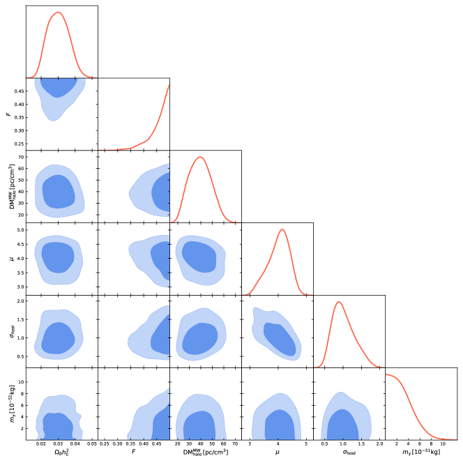
We explore the posterior probability distributions of the free parameters by maximizing the joint likelihood function (Eq. 14) using emcee, an affine-invariant Markov Chain Monte Carlo (MCMC) ensemble sampler implemented in Python (Foreman-Mackey et al., 2013). The free parameters of our model now include the baryon density parameter (where ), the DM contribution from the Milky Way’s halo , the parameters related to the probability distributions for and (i.e., , , and ), and the photon mass . In our MCMC analysis, we set uniform priors on , , , , and . For , we set a Gaussian prior, , within the wide range of . To incorporate the error of the ANN reconstruction into our analysis, at each MCMC step, we sample the Hubble rate function according to the Gaussian distribution with mean and standard deviation . Here is the best-fit function reconstructed by ANN and is the error of the reconstructed function.
The constraint results for these six parameters are summarized in Table 3. For the photon mass , both the and upper limits are presented. Posterior distributions and confidence regions for these parameters are displayed in Fig. 3. Notably, the constraints on are determined as
| (19) |
and
| (20) |
at the and confidence level, respectively. Meanwhile, we find that the baryon density parameter is optimized to be , which is compatible with the value inferred from Planck 2018 () at the confidence level (Planck Collaboration et al., 2020).
To investigate the impact of the prior assumption of on our results, we also perform a parallel comparative analysis of the FRB data using a flat prior on . The corresponding resulting constraints on all parameters are also reported in Table 3. Comparing these inferred parameters with those obtained from the Gaussian prior (see line 1 in Table 3), it is clear that, except for the best-fit value of , the prior assumption of only has a minimal influence on our results.
| Priors of | ||||||
|---|---|---|---|---|---|---|
| Gaussian prior | ||||||
| Flat prior |
IV Discussion and conclusions
As a matter of fact, it is impossible to prove experimentally that the rest mass of a photon is strictly zero. According to the uncertainty principle of quantum mechanics, the ultimately measurable order of magnitude for the photon mass is , where is the reduced Planck constant and is the age of our universe. However, due to the immense importance of Maxwell’s theory and Einstein’s theory of relativity, it is still intellectually stimulating and scientifically significant to approach this ultimate limit by various experiments.
FRBs provide the current best celestial laboratory to test the photon mass via the dispersion method. Constraining with cosmological FRBs, however, one has to know the cosmic expansion rate . In all previous studies, the required information is estimated within the standard CDM cosmological model. Such estimations would involve a circularity problem in constraining , since CDM itself is built on the framework of GR and GR embraces the postulate of the constancy of light speed. In this work, aiming to overcome the circularity problem, we have employed an ANN technology to reconstruct a cosmology-independent function from the discrete CC data.
By combining the DM– measurements of 32 localized FRBs with the reconstructed function from 34 CC data, we have placed the first cosmology-independent photon mass limit. Our results show that the and confidence-level upper limits on the photon mass are (or equivalently ) and (or equivalently ), respectively. Previously, under the assumption of fiducial CDM cosmology, Ref. (Wang et al., 2021) obtained an upper limit of at the confidence level by using a catalog of 129 FRBs (most of them without redshift measurement, and the observed values were used to estimate the pseudo redshifts). Ref. (Lin et al., 2023) obtained () by analyzing a sample of 17 localized FRBs in the flat CDM model. Ref. (Wang et al., 2023) obtained () for flat CDM using a sample of 23 localized FRBs. Despite not assuming a specific cosmological model, the precision of our constraint from 32 localized FRBs is comparable to these previous results. Most importantly, this highlights the validity of our approach and suggests that as the number of CC measurements increases, we can expect even more reliable model-independent tests of the photon mass.
Acknowledgements.
We are grateful to the anonymous referees for their helpful comments. This work is partially supported by the National SKA Program of China (2022SKA0130100), the National Natural Science Foundation of China (grant Nos. 12373053, 12321003, and 12041306), the Key Research Program of Frontier Sciences (grant No. ZDBS-LY-7014) of Chinese Academy of Sciences, International Partnership Program of Chinese Academy of Sciences for Grand Challenges (114332KYSB20210018), the CAS Project for Young Scientists in Basic Research (grant No. YSBR-063), the CAS Organizational Scientific Research Platform for National Major Scientific and Technological Infrastructure: Cosmic Transients with FAST, and the Natural Science Foundation of Jiangsu Province (grant No. BK20221562).References
- De Broglie (1922) L. De Broglie, J. Phys. Radium 3, 422 (1922).
- Proca (1936) A. Proca, J. Phys. Radium 7 7, 347 (1936).
- Kouwn et al. (2016) S. Kouwn, P. Oh, and C.-G. Park, Phys. Rev. D 93, 083012 (2016), arXiv:1512.00541 [astro-ph.CO] .
- Spallicci et al. (2021) A. D. A. M. Spallicci, J. A. Helayël-Neto, M. López-Corredoira, and S. Capozziello, European Physical Journal C 81, 4 (2021), arXiv:2011.12608 [astro-ph.CO] .
- Williams et al. (1971) E. R. Williams, J. E. Faller, and H. A. Hill, Phys. Rev. Lett. 26, 721 (1971).
- Lakes (1998) R. Lakes, Phys. Rev. Lett. 80, 1826 (1998).
- Luo et al. (2003) J. Luo, L.-C. Tu, Z.-K. Hu, and E.-J. Luan, Phys. Rev. Lett. 90, 081801 (2003).
- Lowenthal (1973) D. D. Lowenthal, Phys. Rev. D 8, 2349 (1973).
- Chibisov (1976) G. V. Chibisov, Uspekhi Fizicheskikh Nauk 119, 551 (1976).
- Ryutov (1997) D. D. Ryutov, Plasma Physics and Controlled Fusion 39, A73 (1997).
- Ryutov (2007) D. D. Ryutov, Plasma Physics and Controlled Fusion 49, B429 (2007).
- Liu and Shao (2012) L.-X. Liu and C.-G. Shao, Chinese Physics Letters 29, 111401 (2012).
- Retinò et al. (2016) A. Retinò, A. D. A. M. Spallicci, and A. Vaivads, Astroparticle Physics 82, 49 (2016), arXiv:1302.6168 [hep-ph] .
- Davis et al. (1975) J. Davis, L., A. S. Goldhaber, and M. M. Nieto, Phys. Rev. Lett. 35, 1402 (1975).
- Yang and Zhang (2017) Y.-P. Yang and B. Zhang, Astrophys. J. 842, 23 (2017), arXiv:1701.03034 [astro-ph.HE] .
- Tu et al. (2005a) L.-C. Tu, H.-L. Ye, and J. Luo, Chinese Physics Letters 22, 3057 (2005a).
- Tu et al. (2005b) L.-C. Tu, J. Luo, and G. T. Gillies, Reports on Progress in Physics 68, 77 (2005b).
- Wu et al. (2016) X.-F. Wu, S.-B. Zhang, H. Gao, et al., Astrophys. J. Lett. 822, L15 (2016), arXiv:1602.07835 [astro-ph.HE] .
- Bonetti et al. (2016) L. Bonetti, J. Ellis, N. E. Mavromatos, et al., Physics Letters B 757, 548 (2016), arXiv:1602.09135 [astro-ph.HE] .
- Bonetti et al. (2017) L. Bonetti, J. Ellis, N. E. Mavromatos, et al., Physics Letters B 768, 326 (2017), arXiv:1701.03097 [astro-ph.HE] .
- Shao and Zhang (2017) L. Shao and B. Zhang, Phys. Rev. D 95, 123010 (2017), arXiv:1705.01278 [hep-ph] .
- Xing et al. (2019) N. Xing, H. Gao, J.-J. Wei, et al., Astrophys. J. Lett. 882, L13 (2019), arXiv:1907.00583 [astro-ph.HE] .
- Wei and Wu (2020) J.-J. Wei and X.-F. Wu, Research in Astronomy and Astrophysics 20, 206 (2020), arXiv:2006.09680 [astro-ph.HE] .
- Wang et al. (2021) H. Wang, X. Miao, and L. Shao, Physics Letters B 820, 136596 (2021), arXiv:2103.15299 [astro-ph.HE] .
- Chang et al. (2023) C.-M. Chang, J.-J. Wei, S.-b. Zhang, and X.-F. Wu, JCAP 2023, 010 (2023), arXiv:2207.00950 [astro-ph.HE] .
- Lin et al. (2023) H.-N. Lin, L. Tang, and R. Zou, Mon. Not. R. Astron. Soc. 520, 1324 (2023), arXiv:2301.12103 [gr-qc] .
- Wang et al. (2023) B. Wang, J.-J. Wei, X.-F. Wu, and M. López-Corredoira, JCAP 2023, 025 (2023), arXiv:2304.14784 [astro-ph.HE] .
- Wang et al. (2024) Y.-B. Wang, X. Zhou, A. Kurban, and F.-Y. Wang, Astrophys. J. 965, 38 (2024), arXiv:2403.06422 [astro-ph.HE] .
- Lorimer and Kramer (2012) D. R. Lorimer and M. Kramer, Handbook of Pulsar Astronomy (2012).
- Bentum et al. (2017) M. J. Bentum, L. Bonetti, and A. D. Spallicci, Advances in Space Research 59, 736 (2017).
- Shao and Zhang (2017) L. Shao and B. Zhang, Phys. Rev. D 95, 123010 (2017).
- Cordes and Lazio (2002) J. M. Cordes and T. J. W. Lazio, arXiv e-prints , astro-ph/0207156 (2002), arXiv:astro-ph/0207156 [astro-ph] .
- Prochaska and Zheng (2019) J. X. Prochaska and Y. Zheng, Mon. Not. R. Astron. Soc. 485, 648 (2019), arXiv:1901.11051 [astro-ph.GA] .
- Keating and Pen (2020) L. C. Keating and U.-L. Pen, Mon. Not. R. Astron. Soc. 496, L106 (2020), arXiv:2001.11105 [astro-ph.GA] .
- Wu et al. (2022) Q. Wu, G.-Q. Zhang, and F.-Y. Wang, Mon. Not. R. Astron. Soc. 515, L1 (2022), arXiv:2108.00581 [astro-ph.CO] .
- Deng and Zhang (2014) W. Deng and B. Zhang, Astrophys. J. Lett. 783, L35 (2014), arXiv:1401.0059 [astro-ph.HE] .
- Fukugita et al. (1998) M. Fukugita, C. J. Hogan, and P. J. E. Peebles, Astrophys. J. 503, 518 (1998), arXiv:astro-ph/9712020 [astro-ph] .
- Miralda-Escudé et al. (2000) J. Miralda-Escudé, M. Haehnelt, and M. J. Rees, Astrophys. J. 530, 1 (2000), arXiv:astro-ph/9812306 [astro-ph] .
- Macquart et al. (2020) J. P. Macquart, J. X. Prochaska, M. McQuinn, et al., Nature (London) 581, 391 (2020), arXiv:2005.13161 [astro-ph.CO] .
- McQuinn (2014) M. McQuinn, Astrophys. J. Lett. 780, L33 (2014), arXiv:1309.4451 [astro-ph.CO] .
- Seikel et al. (2012) M. Seikel, C. Clarkson, and M. Smith, JCAP 2012, 036 (2012), arXiv:1204.2832 [astro-ph.CO] .
- Wei and Wu (2017) J.-J. Wei and X.-F. Wu, Astrophys. J. 838, 160 (2017), arXiv:1611.00904 [astro-ph.CO] .
- Wang et al. (2017) G.-J. Wang, J.-J. Wei, Z.-X. Li, et al., Astrophys. J. 847, 45 (2017), arXiv:1709.07258 [astro-ph.CO] .
- Wang et al. (2020) G.-J. Wang, X.-J. Ma, S.-Y. Li, and J.-Q. Xia, Astrophys. J. Suppl. Ser. 246, 13 (2020), arXiv:1910.03636 [astro-ph.CO] .
- Wasserman et al. (2001) L. Wasserman, C. J. Miller, R. C. Nichol, et al., arXiv e-prints , astro-ph/0112050 (2001), arXiv:astro-ph/0112050 [astro-ph] .
- Ioffe and Szegedy (2015) S. Ioffe and C. Szegedy, arXiv e-prints , arXiv:1502.03167 (2015), arXiv:1502.03167 [cs.LG] .
- Clevert et al. (2015) D.-A. Clevert, T. Unterthiner, and S. Hochreiter, arXiv e-prints , arXiv:1511.07289 (2015), arXiv:1511.07289 [cs.LG] .
- Kingma and Ba (2014) D. P. Kingma and J. Ba, arXiv e-prints , arXiv:1412.6980 (2014), arXiv:1412.6980 [cs.LG] .
- Jimenez et al. (2003) R. Jimenez, L. Verde, T. Treu, and D. Stern, Astrophys. J. 593, 622 (2003), arXiv:astro-ph/0302560 [astro-ph] .
- Simon et al. (2005) J. Simon, L. Verde, and R. Jimenez, Phys. Rev. D 71, 123001 (2005), arXiv:astro-ph/0412269 [astro-ph] .
- Stern et al. (2010) D. Stern, R. Jimenez, L. Verde, et al., JCAP 2010, 008 (2010), arXiv:0907.3149 [astro-ph.CO] .
- Moresco et al. (2012) M. Moresco, A. Cimatti, R. Jimenez, et al., JCAP 2012, 006 (2012), arXiv:1201.3609 [astro-ph.CO] .
- Zhang et al. (2014) C. Zhang, H. Zhang, S. Yuan, et al., Research in Astronomy and Astrophysics 14, 1221-1233 (2014), arXiv:1207.4541 [astro-ph.CO] .
- Moresco (2015) M. Moresco, Mon. Not. R. Astron. Soc. 450, L16 (2015), arXiv:1503.01116 [astro-ph.CO] .
- Moresco et al. (2016) M. Moresco, L. Pozzetti, A. Cimatti, et al., JCAP 2016, 014 (2016), arXiv:1601.01701 [astro-ph.CO] .
- Ratsimbazafy et al. (2017) A. L. Ratsimbazafy, S. I. Loubser, S. M. Crawford, et al., Mon. Not. R. Astron. Soc. 467, 3239 (2017), arXiv:1702.00418 [astro-ph.CO] .
- Borghi et al. (2022) N. Borghi, M. Moresco, and A. Cimatti, Astrophys. J. Lett. 928, L4 (2022), arXiv:2110.04304 [astro-ph.CO] .
- Jiao et al. (2023) K. Jiao, N. Borghi, M. Moresco, and T.-J. Zhang, Astrophys. J. Suppl. Ser. 265, 48 (2023), arXiv:2205.05701 [astro-ph.CO] .
- Tomasetti et al. (2023) E. Tomasetti, M. Moresco, N. Borghi, et al., Astron. & Astrophys. 679, A96 (2023), arXiv:2305.16387 [astro-ph.CO] .
- Gaztañaga et al. (2009) E. Gaztañaga, A. Cabré, and L. Hui, Mon. Not. R. Astron. Soc. 399, 1663 (2009), arXiv:0807.3551 [astro-ph] .
- Blake et al. (2012) C. Blake, S. Brough, M. Colless, et al., Mon. Not. R. Astron. Soc. 425, 405 (2012), arXiv:1204.3674 [astro-ph.CO] .
- Samushia et al. (2013) L. Samushia, B. A. Reid, M. White, et al., Mon. Not. R. Astron. Soc. 429, 1514 (2013), arXiv:1206.5309 [astro-ph.CO] .
- Jimenez and Loeb (2002) R. Jimenez and A. Loeb, Astrophys. J. 573, 37 (2002), arXiv:astro-ph/0106145 [astro-ph] .
- Bentum et al. (2017) M. J. Bentum, L. Bonetti, and A. D. A. M. Spallicci, Advances in Space Research 59, 736 (2017), arXiv:1607.08820 [astro-ph.IM] .
- Planck Collaboration et al. (2020) Planck Collaboration et al., Astron. & Astrophys. 641, A6 (2020), arXiv:1807.06209 [astro-ph.CO] .
- Law et al. (2023) C. J. Law, K. Sharma, V. Ravi, et al., arXiv e-prints , arXiv:2307.03344 (2023), arXiv:2307.03344 [astro-ph.HE] .
- Chatterjee et al. (2017) S. Chatterjee, C. J. Law, R. S. Wharton, et al., Nature (London) 541, 58 (2017), arXiv:1701.01098 [astro-ph.HE] .
- Bhandari et al. (2022) S. Bhandari, K. E. Heintz, K. Aggarwal, et al., Astron. J. 163, 69 (2022), arXiv:2108.01282 [astro-ph.HE] .
- Marcote et al. (2020) B. Marcote, K. Nimmo, J. W. T. Hessels, et al., Nature (London) 577, 190 (2020), arXiv:2001.02222 [astro-ph.HE] .
- Bannister et al. (2019) K. W. Bannister, A. T. Deller, C. Phillips, et al., Science 365, 565 (2019), arXiv:1906.11476 [astro-ph.HE] .
- Prochaska et al. (2019) J. X. Prochaska, J.-P. Macquart, M. McQuinn, et al., Science 366, 231 (2019), arXiv:1909.11681 [astro-ph.GA] .
- Bhandari et al. (2020) S. Bhandari, E. M. Sadler, J. X. Prochaska, et al., Astrophys. J. Lett. 895, L37 (2020), arXiv:2005.13160 [astro-ph.GA] .
- Ravi et al. (2019) V. Ravi, M. Catha, L. D’Addario, et al., Nature (London) 572, 352 (2019), arXiv:1907.01542 [astro-ph.HE] .
- Chittidi et al. (2021) J. S. Chittidi, S. Simha, A. Mannings, et al., Astrophys. J. 922, 173 (2021), arXiv:2005.13158 [astro-ph.GA] .
- Heintz et al. (2020) K. E. Heintz, J. X. Prochaska, S. Simha, et al., Astrophys. J. 903, 152 (2020), arXiv:2009.10747 [astro-ph.GA] .
- Law et al. (2020) C. J. Law, B. J. Butler, J. X. Prochaska, et al., Astrophys. J. 899, 161 (2020), arXiv:2007.02155 [astro-ph.HE] .
- Ravi et al. (2022) V. Ravi, C. J. Law, D. Li, et al., Mon. Not. R. Astron. Soc. 513, 982 (2022), arXiv:2106.09710 [astro-ph.HE] .
- James et al. (2022) C. W. James, E. M. Ghosh, J. X. Prochaska, et al., Mon. Not. R. Astron. Soc. 516, 4862 (2022), arXiv:2208.00819 [astro-ph.CO] .
- Ryder et al. (2022) S. D. Ryder, K. W. Bannister, S. Bhandari, et al., arXiv e-prints , arXiv:2210.04680 (2022), arXiv:2210.04680 [astro-ph.HE] .
- Foreman-Mackey et al. (2013) D. Foreman-Mackey, D. W. Hogg, D. Lang, and J. Goodman, Pub. Astro. Soc. Pacific 125, 306 (2013), arXiv:1202.3665 [astro-ph.IM] .