Evolution of random representable matroids: minors, circuits, connectivity and the critical number

Abstract

We study the evolution of random matroids represented by the sequence of random matrices over $\mathbb{F}_{q}$ where columns are added one after the other, and each column vector is a uniformly random vector in $\mathbb{F}_{q}^{n}$, independent of each other. We study the appearance of matroid minors, the appearance of circuits, the evolution of the connectivities and the critical number. We settle several open problems in the literature.

1 Introduction

Random graphs were first introduced by Erdős and Rényi [6] in 1959, and in particular they studied the evolution of random graphs by studying a random process of graphs on a set of $n$ vertices, where the edges are added one after the other in the process. The most astonishing phenomenon in the study of random graph evolution is the characterisation of phase transitions of various (often increasing) graph properties. For instance, initially, the graph is acyclic with each component being a tree of bounded order. Then, small cycles may start to appear whereas each component remains in small size and contains at most one cycle. At the time where the number of edges is around $n/2$, small components start to rapidly connect to each other and form a giant component in which more complicated graph structures start to appear. Long cycles and graph minors of fixed sizes simultaneously appear at the time the giant component emerges. Other well studied graph properties and graph parameters include connectivity, Hamiltonicity, the appearance of given subgraphs, chromatic number, etc.

The Erdős-Rényi graph process immediately induces a random process on graphical matroids, which motivates the generalisations to other classes of random matroid processes. One generalisation is to consider the matroids represented by the incidence matrices of random uniform hypergraphs, which was introduced by Cooper, Frieze and Pegden [4], and was more formally described and studied as an evolutionary random process in [7]. The other generalisation is to consider uniformly random vectors over a finite field and add them one after the other independently, and consider the random matroids represented by these matrices. This model was first introduced by Kelly and Oxley [9, 10]. In their model, they consider random subsets of the elements in the complete projective geometry $PG(n-1,q)$ where $q$ is a prime power. Two related models were introduced and studied. In the first one, $PG(n-1,q;p)$ where $p\in[0,1]$, every element in $PG(n-1,q)$ is kept independently with probability $p$. In the second model $PG(n-1,q;m)$ where $m$ is an integer between 0 and $(q^{n}-1)/(q-1)$, a uniformly random subset of $m$ elements of $PG(n-1,q)$ is selected. Obviously, $PG(n-1,q;p)$ and $PG(n-1,q;m)$ are analogs of ${\mathcal{G}}(n,p)$ and ${\mathcal{G}}(n,m)$ for random graphs, and $PG(n-1,q;m)$ is precisely $PG(n-1,q;p)$ conditioned to $|PG(n-1,q;p)|=m$; i.e. exactly $m$ elements are selected. After that, Kordecki [12, 13], Kordecki and Luczak [14, 15] further studied matroid properties of these models, including circuits, connectivity, and submatroids, etc. Soon after the introduction of $PG(n-1,q;m)$ and $PG(n-1,q;p)$, Kelly and Oxley [8] introduced a slightly different model $M([U_{q}]_{n\times m})$. In this model, $[U_{q}]_{n\times m}$ is a uniformly random $n\times m$ matrix over $\mathbb{F}_{q}$, and $M([U_{q}]_{n\times m})$ is the matroid represented by $[U_{q}]_{n\times m}$. Due to the independence of the column vectors, $[U_{q}]_{n\times m}$ is a little easier to analyse than $PG(n-1,q;p)$ and $PG(n-1,q;m)$. Indeed, as noted by all the authors that followed this study, these three models are asymptotically equivalent for all the problems (e.g. rank, circuits and connectivity) they were studying. We give a proof of their equivalence in Proposition 1 below.

In this paper, we use the last model introduced by Kelly and Oxley [8], however we stress that columns are added one by one and we are interested in the evolution of the matroids represented by this random process of matrices. Let $\mathbb{F}_{q}$ denote the finite field of order $q$ where $q$ is a prime power. Let ${\boldsymbol{v}}$ be a uniformly random vector in $\mathbb{F}_{q}^{n}$, and let $(v_{i})_{i\geq 1}$ be a sequence of random vectors that are independent copies of ${\boldsymbol{v}}$. Finally, for every $m\geq 1$, let $A_{m}=[v_{1},\ldots,v_{m}]$ be the $n\times m$ matrix formed by including the first $m$ vectors $v_{1},\ldots,v_{m}$ in the sequence, and let $M[A_{m}]$ be the matroid represented by $A_{m}$. Notice that for every $m\geq 1$, $A_{m}$ has the same distribution as $[U_{q}]_{n\times m}$. We study various matroid properties and parameters of $M[A_{m}]$ as $m$ grows. In particular, we take a thorough study of the time when matroid minors of small ranks appear, the appearance of the projective geometry of growing rank of $n$ as a minor, the appearance of the circuits of different lengths, the evolution of the connectivity, and the growth rate of the critical number. We discuss them in turn in the coming subsections. We start our discussions by unifying the notions of the three models $PG(n-1,q;p)$, $PG(n-1,q;m)$ and $M[A_{m}]$ and show their asymptotic equivalence. The following Gaussian binomial coefficients will be used throughout the paper, which counts the $k$-dimensional subspaces of $\mathbb{F}_{q}^{n}$:

$$\genfrac{[}{]}{0.0pt}{}{n}{k}_{q}:=\prod_{i=0}^{k-1}\frac{q^{n-i}-1}{q^{k-i}-1};\quad[n]_{q}:=\genfrac{[}{]}{0.0pt}{}{n}{1}_{q}=\frac{q^{n}-1}{q-1}.$$

Notice that $PG(n-1,q)$ contains exactly $[n]_{q}$ elements. Given a sequence of probability spaces indexed by $n$, we say a sequence of events $A_{n}$ occurs asymptotically almost surely (a.a.s.) if $\lim_{n\to\infty}{\mathbb{P}}(A_{n})=1$. The standard Landau notation and basic matroid notions such as simple matroid, free matroid, and the rank of a matroid will be introduced in Section 2.

Proposition 1.

The three models (M1): $M[A_{m}]$, (M2): $PG(n-1,q;m)$ and (M3): $PG(n-1,q;p)$, are related as follows:

1. (M1), conditioned on the event that $M[A_{m}]$ is simple, is equivalent to (M2).

2. (M3), conditioned on the event that precisely $m$ elements of $PG(n-1,q)$ are included, is equivalent to (M2).

3. If $m=o(q^{n/2})$ then (M1) and (M2) are asymptotically equivalent.

Proof.  Parts (a,b) are obvious. For part (c), suppose that $m=o(q^{n/2})$. By part (i), it suffices to show that a.a.s. $M[A_{m}]$ is simple. The probability that $A_{m}$ has a zero column is at most $mq^{-n}=o(1)$. Each element in $PG(n-1,q)$ corresponds to exactly $q-1$ vectors in $\mathbb{F}_{q}^{n}$. Thus, the probability that $A_{m}$ has two linearly dependent columns is at most $\binom{m}{2}[n]_{q}(q-1)^{2}q^{-2n}=o(1)$. Hence, a.a.s. $M[A_{m}]$ is a simple matroid.    

1.1 Minors

Let $N$ be an $\mathbb{F}_{q}$-representable matroid. Let $\tau_{\texttt{N-minor}}$ be the smallest $m$ such that $M[A_{m}]$ contains $N$ as a minor (the definition of matroid minor is given in Section 2). Altschuler and Yang [1] determined the critical window in which $\tau_{\texttt{N-minor}}$ lies, provided that the size of $N$ is fixed, i.e. independent of $n$. Given a matrix or a matroid $M$, let $\text{{crk}}(M)$ denote the co-rank of $M$. Given a random variable $X_{n}$ and a real number $x_{n}$, we write $X_{n}=O_{p}(x_{n})$ if

$$\lim_{\varepsilon\to 0}\limsup_{n\to\infty}\left({\mathbb{P}}(X_{n}<\varepsilon x_{n})+{\mathbb{P}}(X_{n}>\varepsilon^{-1}x_{n})\right)=0.$$

Theorem 2.

Suppose $N$ is a fixed non-free $\mathbb{F}_{q}$-representable matroid.

1. (Theorems 5 and 6 of [1]) Let $k\geq 0$ be a positive integer. There exist constants $C,D>0$ depending on $N$, $q$ and $k$ such that

   $$\liminf_{n\to\infty}{\mathbb{P}}(\tau_{\texttt{N-minor}}\leq m)>C\quad\text{if }m=n+k\ \text{and}\ k\geq 1$$

   $$\limsup_{n\to\infty}{\mathbb{P}}(\tau_{\texttt{N-minor}}\leq m)\leq D\quad\text{if }m=n-k.$$

2. (Theorems 3 and 8 of [1]) $\tau_{\texttt{N-minor}}=n+O_{p}(1)$.

Note that if $N$ is a free matroid with rank $r$ such that $n-r\to\infty$ then it is easy to see (e.g. it follows easily from the proof of Lemma 22) that a.a.s. all the columns of $A_{r}$ are linearly independent and thus a.a.s. $\tau_{\texttt{N-minor}}=r$. On the other hand, if $N$ is not $\mathbb{F}_{q}$-representable then $N$ can never be a minor of $M[A_{m}]$, no matter how large $m$ is. Therefore, in the discussions of matroid minors we only focus on non-free $\mathbb{F}_{q}$-representable matroid.

Altschuler and Yang gave specific bounds $C,D$ in Theorem 2(a). Interested readers can find them in [1]. We do not express them here, as these bounds only give qualitative information about ${\mathbb{P}}(|\tau_{\texttt{N-minor}}-n|>k)$ for $k\to\infty$, which they used to come to the conclusion of Theorem 2(b). However these bounds give little information about ${\mathbb{P}}(\tau_{\texttt{N-minor}}\leq n+k)$ when $|k|$ is small. Our first result is a strengthening of Theorem 2(a) by providing the precise limiting distribution of $\tau_{\texttt{N-minor}}-n$. For convenience, we define $\sum_{i=j}^{h}a_{i}$ to be 0 and $\prod_{i=j}^{h}a_{i}$ to be 1 if $h<j$ for any sequence of real numbers or real functions $a_{i}$. Given a power series $P(z)$ let $[z^{n}]P(z)$ denote the coefficient of $z^{n}$ in $P(z)$.

Theorem 3.

Let $N$ be a fixed $\mathbb{F}_{q}$-representable matroid and let $r$ and $c$ denote the rank and the co-rank of $N$ respectively. Suppose that $c\geq 1$. Then, for any fixed $k\in{\mathbb{Z}}$,

$$\lim_{n\to\infty}{\mathbb{P}}(\tau_{\texttt{N-minor}}=n+k)=C_{c,k},$$

where $C_{c,k}=0$ if $k>c$; and if $k\leq c$ then

$$C_{c,k} = \beta_{c,k}q^{k-c}\sum_{i=0}^{c-1}\left(\alpha_{c,k,0}+\sum_{i=1}^{c-1}\frac{1}{\prod_{j=1}^{i}(1-q^{-j})}\alpha_{c,k,i}\right),$$

$$\beta_{c,k} = \prod_{j=c+1-k}^{\infty}(1-q^{-j}),$$

$$\alpha_{c,k,i} = [z^{c-1-i}]\prod_{j=0}^{c-k-1}(1-zq^{-j})=(-1)^{c-1-i}\sum_{*}q^{-\sum_{r=1}^{c-1-i}j_{r}},$$

where the summation $\sum_{*}$ in the expression for $\alpha_{c,k,i}$ is over all integers $0\leq j_{1}<j_{2}<\ldots<j_{c-1-i}\leq c-k-1$.

We plot below the limiting point-wise probabilities ${\mathbb{P}}(\tau_{\texttt{N-minor}}=n+k)$ for $k\in[-10,5]$ when $(q,c)=(2,1)$ (the one on the left) and when $(q,c)=(2,2)$ (the one in the middle). The last figure on the right compares the limiting cumulative distribution function ${\mathbb{P}}(\tau_{\texttt{N-minor}}\leq n+k)$, in red dots, with the bounds in Theorem 2(a) by Altschuler and Yang, in green curve. Recall that the bounds in Theorem 2(a) are upper bounds for non-positive $k$ and lower bounds for positive $k$.

Our second result improving over Altschuler and Yang’s is a hitting time result of $\tau_{\texttt{N-minor}}$ when the rank and the co-rank of $N$ are fixed or slowly growing functions of $n$. Let $\tau_{\texttt{crk=c}}$ be the smallest $m$ such that the co-rank of $A_{m}$ is equal to $c$. This is well defined as the co-rank of $A_{m}$ is non-decreasing as $m$ grows.

Theorem 4.

Suppose that $N$ is an $\mathbb{F}_{q}$-representable non-free matroid such that $rq^{rc}=o(n)$, where $r$ and $c$ denote the rank and the co-rank of $N$ respectively. Then a.a.s. $\tau_{\texttt{N-minor}}=\tau_{\texttt{crk=c}}$.

As a direct corollary, we prove that a.a.s. an $N$-minor is formed by step $n+\text{{crk}}(N)$, improving Theorem 2(b). On the other hand, there is a non-vanishing probability that the first $N$-minor is created precisely during the step $n+\text{{crk}}(N)$.

Corollary 5.

Suppose that $N$ is a fixed non-free $\mathbb{F}_{q}$-representable matroid. Let $c$ be the co-rank of $N$. Then, a.a.s. $\tau_{\texttt{N-minor}}=n+O_{p}(1)$. Moreover, letting $\gamma_{q,c}=\prod_{j=c}^{\infty}(1-q^{-j})$, we have

$$\lim_{n\to\infty}{\mathbb{P}}(\tau_{\texttt{N-minor}}\leq n+c)=1;\quad\lim_{n\to\infty}{\mathbb{P}}(\tau_{\texttt{N-minor}}\leq n+c-1)=1-\gamma_{q,c},$$

for every $(q,c)$. Moreover,

$$\lim_{q\to\infty}\gamma_{q,c}=1\quad\mbox{for every $c$};\quad\lim_{c\to\infty}\gamma_{q,c}=1\quad\mbox{for every $q$}.$$

The next corollary shows that $\tau_{\texttt{N-minor}}$ has a 1-point concentration if $|N|$ is not too large, and $\text{{crk}}(N)=\omega(1)$. Here, $|N|$ denotes the size of $N$, which is the number of elements in $N$.

Corollary 6.

Suppose that $N$ is an $\mathbb{F}_{q}$-representable non-free matroid. If $\text{{crk}}(N)=\omega(1)$ and $|N|\leq(2-\varepsilon)\sqrt{\log_{q}n}$ for some fixed $\varepsilon>0$, then a.a.s. $\tau_{\texttt{N-minor}}=n+\text{{crk}}(N)$.

Note that the matroid $N$ in Theorems 2, 3, 4 and Corollaries 5 and 6 is general, and does not need to be simple. In the next corollary of Theorem 4, we generalise Theorem 2 and study $\tau_{\texttt{PGr}}$, the minimum integer $m$ such that $M[A_{m}]$ contains the complete projective geometry $PG(r-1,q)$ as a minor. All the logarithms in the paper are natural logarithms with base $e$, unless otherwise with a specified base.

Theorem 7.

Suppose that $r=\omega(1)$. Let $\zeta=[r]_{q}$.

1. A.a.s. $\tau_{\texttt{PGr}}\leq n+\zeta\log\zeta+\omega(\zeta)$.

2. If $r=\omega(\log n)$ then a.a.s. $\tau_{\texttt{PGr}}\sim\zeta\log\zeta$.

3. If $N$ is an $\mathbb{F}_{q}$-representable simple non-free matroid with rank $r\leq\alpha\log n$ for any fixed $\alpha<1/\log q$ then a.a.s. $\tau_{\texttt{N-minor}}\sim n$.

Remark 8.

Theorem 7 determines the asymptotic value of $\tau_{PGr}$ provided that $r\leq(1-\varepsilon)\log_{q}n$ for some fixed $\varepsilon>0$, or $r=\omega(\log n)$. However, we did not manage to prove a lower bound for $\tau_{PGr}$ that matches its upper bound in Theorem 7(a) for $\log_{q}n\leq r=\Theta(\log n)$. There is a trivial lower bound $n+\zeta-r=n+(1+o(1))\zeta$, since the co-rank of $A_{m}$ must be at least the co-rank of $PG(r-1,q)$ (see Lemma 23 below). It is possible that in the range $\log_{q}n\leq r=\Theta(\log n)$, both the upper bound (Theorem 7(a)) and the lower bound ($n+(1+o(1))\zeta$) are not tight.

The proofs of Theorems 3, 4 and 7, and the proofs of Corollaries 5 and 6 will be presented in Section 3.

1.2 Circuits

The circuits in a matroid (see its formal definition in Section 2) are minimal dependent subsets and are analogs of cycles in a graph. The appearance of the circuits with constant length has been studied by Kelly and Oxley [8], whereas the longer circuits were investigated by Kordecki and Łuczak [15]. We collect and restate their results in the following theorem.

Theorem 9.

1. (Theorem 5.1 of [8]) Suppose that $k=o(m)$ and that $m^{k}q^{-n}$ is bounded. Then

   $$\Pr(M[A_{m}]\text{has no $k$-circuits})\sim\exp\left(-\frac{(q-1)^{k-1}}{k!}\frac{m^{k}}{q^{n}}\right).$$

2. (Theorem 6 of [15]) For each $1\leq k\leq n+1$, let $\mu_{k}=\binom{m}{k}(q-1)^{k}q^{-n}.$

   1. If $\mu_{k}\to 0$, then a.a.s. $M[A_{m}]$ does not contain a $k$-circuit.

   2. If $\mu_{k}\to\infty$ and either $n-k\to\infty$ or $k(m-k)/m\to\infty$, then a.a.s. $M[A_{m}]$ contains a $k$-circuit.

Remark 10.

Kordecki and Łuczak’s result [15] was proved for $PG(n-1,q;m)$. The same holds for $M[A_{m}]$ by Proposition 1. The original statement of [15, Theorem 6] was slightly stronger, by considering the appearance of circuits whose lengths lie in a specified interval. For simplicity we stated a simplified version. The value $\mu_{k}$ is the asymptotic number of circuits with length $k$ in $PG(n-1,q;m)$ and $M[A_{m}]$.

Theorem 9 provides the full information on the types of circuits that are likely or unlikely to appear in $M[A_{m}]$ for every $m$. We give a few interesting corollaries of Theorem 9 in terms of $\tau_{\texttt{k-circ}}$, the minimum integer $m$ such that $M[A_{m}]$ has a circuit with length $k$. Given $0<a\leq 1$, define

$$g_{a}(y)=y\log y+a\log(q-1)-a\log a-(y-a)\log(y-a)-\log q,\quad\text{for}\ y\geq a,$$ (1)

where $0\log 0$ is defined to be 0 so that $g_{a}(y)$ is continuous at $y=a$.

Corollary 11.

1. Let $k$ be a fixed positive integer. Then, $\tau_{\texttt{k-circ}}=\Theta_{p}(q^{n/k})$.

2. If $k\to\infty$ and $k=o(n)$ then a.a.s. $\tau_{\texttt{k-circ}}\sim\frac{1}{e(q-1)}kq^{n/k}$.

3. If $k\sim an$ for some fixed $0<a\leq 1$ then $g_{a}(y)$ has a unique root $b$, and a.a.s. $\tau_{\texttt{k-circ}}\sim bn$.

Remark 12.

For $0<a\leq 1$, let $b=b(a)$ be the unique root of $g_{a}(y)$. Then $b$ is strictly convex and has a minimum value of $1$, achieved at $a^{*}:=\frac{q-1}{q}$. Moreover, $b(1)<2$ and $b(a)\to\infty$ as $a\to 0$.

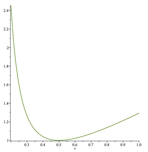
Figure 1: Plot of $b(a)$

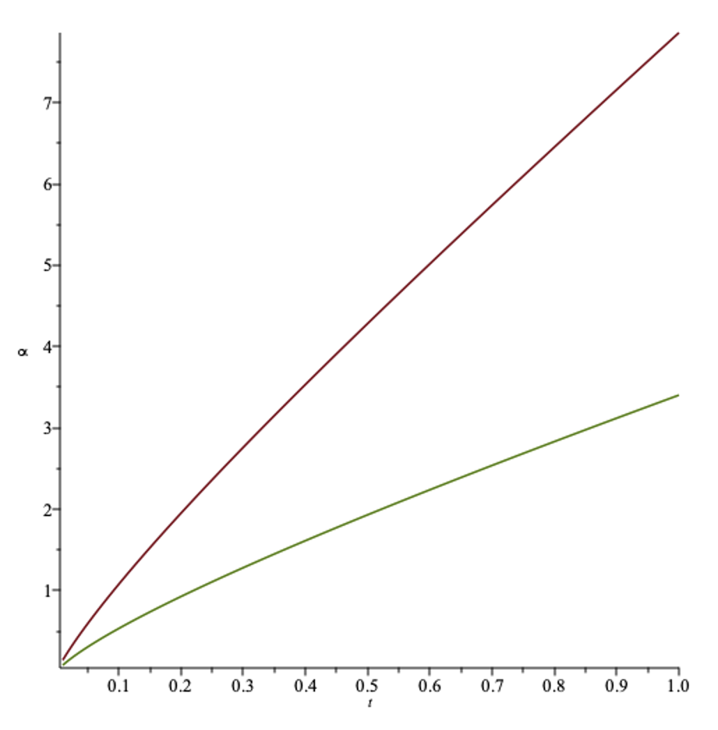
Figure 2: Upper bound of $\alpha$ from Kelly and Oxley and our lower bound

Remark 12 follows from simple calculus and we include its proof in the Appendix for interested readers. A plot of $b(a)$ for $q=2$ is given below in Figure 1. Following Remark 12 we immediately obtain the following interesting corollary about the length of the first appearing circuit and the appearing time of the first Hamilton circuit (i.e. the circuit with length $n$).

Corollary 13.

1. The first circuit appearing in $M[A_{m}]$ has length asymptotic to $(1-q^{-1})n$;

2. The first Hamilton circuit appears in less than $2n$ steps for every finite field $\mathbb{F}_{q}$.

The proofs for Corollaries 11 and 13 are given in Section 4.

1.3 Connectivity

The concept of vertex-connectivity in graphs generalizes naturally to matroids. It is easily seen that a graph $G$ is $k$-vertex-connected if and only if it is not the union of two edge-disjoint subgraphs $G_{1},G_{2}$ such that $\min\{|V(G_{1})|,|V(G_{2})|\}>k$, and $|V(G_{1})\cap V(G_{2})|<k$; the latter is equivalent to $|V(G_{1})|+|V(G_{2})|-|V(G)|<k$.

Analogously, a vertical $k$-separation in a matroid $M$ is a partition $(A_{1},A_{2})$ of $M$ so that

1. $\min\{\text{{rk}}(A_{1}),\text{{rk}}(A_{2})\}\geq k$, and

2. $\text{{rk}}(A_{1})+\text{{rk}}(A_{2})-\text{{rk}}(M)\leq k-1$.

The vertical connectivity $\kappa(M)$ is defined to be the smallest $k$ such that $M$ has a vertical $k$-separation. It may be the case that $M$ has no vertical $k$-separations for any $k$, in which case $\kappa(M)=\infty$; this holds, for instance, if $M={\mathbb{F}}_{q}^{n}$.

From the perspective of graph theory, this is the most natural notion of matroid connectivity; indeed, if $G$ is a graph with no isolated vertex, then the value of $\kappa$ for the graphic matroid $M(G)$ is equal to the vertex connectivity of $G$: see [21], Theorem 8.6.1. (Incidentally, this fact is the reason for the unnatural-looking offset by one in condition ii).

However, $\kappa$ fails to have a certain natural matroid property: invariance under duality. Each matroid $M$ has a dual matroid $M^{*}$, and the relationship between $M$ and $M^{*}$ is crucial in much of matroid theory – for instance, we have $M^{**}=M$, and matroid duality agrees with planar duality in the case of the graphic matroids of planar graphs. It is not necessary here to discuss matroid duality in detail, but we comment that the rank function of the dual matroid is given by $\text{{rk}}^{*}(X)=|X|+\text{{rk}}(E(M)\setminus X)-\text{{rk}}(M)$ (see [21], Proposition 2.1.9).

In general, we have $\kappa(M)\neq\kappa(M^{*})$, so vertical connectivity has a dual notion. A cyclic $k$-separation of $M$ is a vertical $k$-separation of $M^{*}$, and the cyclic connectivity $\kappa^{*}(M)$ is the smallest $k$ such that $M$ has a cyclic $k$-separation. Similarly as before, $\kappa^{*}(M)$ defined to be $\infty$ if no cyclic separation exists. Using the above formula for the dual rank function, one can easily show that a partition $(A_{1},A_{2})$ of $M$ is a cyclic $k$-separation of $M$ if and only if

1. $\text{{rk}}(A_{i})<|A_{i}|$ for each $i$, and

2. $\text{{rk}}(A_{1})+\text{{rk}}(A_{2})-\text{{rk}}(M)\leq k-1$.

Condition i can be replaced with the requirement that $A_{1}$ and $A_{2}$ are dependent, or by the condition $\min(\text{{rk}}^{*}(A_{1}),\text{{rk}}^{*}(A_{2}))\geq k$. It is harder to relate this intuitively to graphs, except to comment that, if $M$ is the graphic matroid of a planar graph $G$, then the cyclic connectivity of $M$ is the vertex connectivity of a planar dual of $G$. One way to construct a small cyclic separation in a matroid $M$ is simply to take a small circuit; if $C$ is a circuit of $M$ for which $E(M)\setminus C$ is a dependent set, then $(C,E(M)\setminus C)$ satisfies i, and $\text{{rk}}(C)+(\text{{rk}}(E(M)\setminus C)-\text{{rk}}(M))\leq|C|-1+0$, so $C$ gives a cyclic $|C|$-separation, implying that $\kappa^{*}(M)\leq|C|$. In the setting of planar duality, this corresponds to a fact that a small cycle in the planar dual of $G$ gives rise to a small cut in $G$.

Evidently cyclic connectivity is not invariant under matroid duality. However, there is a third notion of connectivity that is. A Tutte $k$-separation of $M$ is a partition $(A_{1},A_{2})$ of $M$ so that

1. $\min\{|A_{1}|,|A_{2}|\}\geq k$, and

2. $\text{{rk}}(A_{1})+\text{{rk}}(A_{2})-\text{{rk}}(M)<k-1$.

The Tutte connectivity $t(M)$ is the smallest $k$ so that $G$ is Tutte $k$-connected. Each cyclic or vertical $k$-separation is also a Tutte $k$-separation, which implies that $t(M)\leq\min(\kappa(M),\kappa^{*}(M))$. In fact, one can show that if $|M|\geq 3$ and $t(M)<\infty$, then there is always either a vertical or a cyclic $t(M)$-separation, which implies that equality holds. This fact is essentially stated in [21], Proposition 8.6.6, but the notation is slightly different from ours in edge cases, as $\kappa(M)$ and $\kappa^{*}(M)$ are defined in [21] to always be finite.

Proposition 14.

If $M$ is a matroid with $|M|\geq 3$, then $t(M)=\min\{\kappa(M),\kappa^{*}(M)\}$.

This fact shows that Tutte connectivity is invariant under matroid duality, so in a sense it is the most natural connectivity notion of the three; usually the unadorned ‘connectivity’ of a matroid refers to the Tutte connectivity.

The girth $\operatorname{gir}(M)$ of a matroid $M$ is the size of a smallest circuit of $M$, or $\infty$ if $M$ is independent. We have seen that in nontrivial cases, small circuits give small cyclic separations. It follows that the girth usually provides an upper bound for the connectivity of a matroid. The following bound ([21], Theorem 8.6.4) will be useful.

Proposition 15.

If $M$ is a matroid that is not a uniform matroid $U_{r,n}$ with $n\geq 2r-1$, then $t(M)=\min(\kappa(M),\operatorname{gir}(M))$.

A striking difference between matroid and graph connectivities is the monotonicity. From the definitions it is easy to see that all of the Tutte, the vertical, and the cyclic connectivities are not monotone; i.e. adding elements to a matroid may decrease the connectivity. Our first observation is that $\kappa(M[A_{m}])$ is a.a.s. monotonely non-decreasing as $m$ grows. On the other hand, the Tutte connectivity first follows $\kappa(M[A_{m}])$, and then after some linear number of steps, it becomes governed by $\text{gir}(M[A_{m}])$ and decreases as $m$ grows. The evolutionay trajectory of $\kappa^{*}(M[A_{m}])$ is very different from $\kappa(M[A_{m}])$, which starts from $\infty$ and in the end is governed by $\text{gir}(M[A_{m}])$. We will study $\kappa^{*}(M[A_{m}])$ in a different paper.

Theorem 16.

1. A.a.s. $\kappa(M[A_{m}])$ is monotonely non-decreasing as $m$ increases.

2. A.a.s. $t(M[A_{m}])=\kappa(M[A_{m}])$ for all $m=n+o(n)$.

3. A.a.s. there exists $\hat{m}=\Theta(n)$ such that $t(M[A_{m}])=\kappa(M[A_{m}])$ for all $m<\hat{m}$, and $t(M[A_{m}])<\kappa(M[A_{m}])$ for all $m\geq\hat{m}$.

Thanks to the monotonicity of the vertical connectivity of $M[A_{m}]$ as shown in Theorem 16(a), it is natural to define $\tau_{\text{k-conn}}$ to be the smallest $m$ such that $M[A_{m}]$ is vertically $k$-connected. Due to Proposition 15 and our good understanding of $\tau_{\texttt{k-circ}}$ from Corollary 11, $\tau_{\text{k-conn}}$ and $\tau_{\texttt{k-circ}}$ together would immediately determine the evolution of $t(M[A_{m}])$. The limiting distribution of $\tau_{\text{k-conn}}$ has been determined by Kordecki and Łuczak [15] when $k$ is a constant; whereas an upper bound on $\tau_{\text{k-conn}}$ was provided by Kelly and Oxley [8] when $k$ is linear in $n$.

Theorem 17.

[15, Theorem 4] Let $k\geq 2$ and $m-n-(k-1)\log_{q}n\to c$ for some constant $c$. Then

$$\lim_{n\to\infty}{\mathbb{P}}\big{(}M[A_{m}]\text{ is $k$-connected}\big{)}=\exp\big{(}-(q-1)^{k-2}q^{-c}/(k-1)!\big{)}.$$

Kelly and Oxley give the following upper bounds for when $M[A_{n\times m}]$ becomes $k$-connected.

Theorem 18.

1. ([8, Theorem 4.4]) A.a.s. $\kappa(M[A_{m}])=\infty$ if $m\geq(1+\alpha)n$ where $\alpha$ is any constant such that

   $$\alpha>\frac{\log(2q-1)}{2\log q-\log(2q-1)}.$$

2. ([8, Theorem 4.5] ) Suppose that $k\sim tn$ for some fixed $0<t<1$ then a.a.s. $\tau_{\text{k-conn}}\leq(1+\alpha)n$ for any constant $\alpha$ such that

   $$t\log\left[\frac{(1+t)\alpha}{t^{2}}\right]<(\alpha-t)\ln q-2t.$$

Our contributions are the determination of the sharp phase transition of $\tau_{\text{k-conn}}$ for all $k=o(n)$, and a lower bound on $\tau_{\text{k-conn}}$ for $k=\Theta(n)$.

Theorem 19.

1. Suppose $k\to\infty$ and $k=o(n)$. Then, a.a.s. $\tau_{\text{k-conn}}-n\sim k\log_{q}(n/k)$.

2. Suppose that $k\sim tn$ for some fixed $0<t<1$. Then, a.a.s. $\tau_{\text{k-conn}}\geq(1+\alpha)n$ where $\alpha$ is any constant satisfying the following.

   $$t\log\frac{1+\alpha}{t}+(1+\alpha-t)\log\frac{1+\alpha}{1+\alpha-t}+t\log(q-1)-\alpha\log q>0.$$ (2)

Our lower bound on $\tau_{\text{k-conn}}$ for linear $k$ does not match the upper bound in Theorem 18. See Figure 2 for the plot in which we compare the upper bounds by Kelly and Oxley and the lower bounds in Theorem 19(b); the horizontal axis is for $t=k/n$, and the vertical axis is for $n^{-1}\tau_{\text{k-conn}}-1$. Determining the asymptotic value of $\tau_{\text{k-conn}}$ for $k=\Theta(n)$ is an interesting open problem.

The proofs for Theorems 16 and 19 will be given in Section 5.

1.4 Critical number

The critical number is an extension of the notion of the chromatic number of graphs to matroids. It is easy to see that a graph $G$ is $2^{k}$-colourable if and only if $E(G)$ is the union of $k$ edge cuts of $G$. For each set $U\subseteq V(G)$, the edge cut $\delta(U)$ corresponds to the set of support-$2$ vectors in ${\mathbb{F}}_{2}^{V}$ that have a nonzero dot product with the characteristic vector $1_{U}$. Hence, we can form an analogue of chromatic number by defining $\chi_{q}(M)$ for each matroid $M\subseteq{\mathbb{F}}_{q}^{n}$ to be the minimum $k$ such that there are vectors $v_{1},\dotsc,v_{k}\in{\mathbb{F}}_{q}^{n}$ such that, for all $w\in M$, the dot product $w^{T}v_{i}$ is nonzero for some $i\in[k]$. In other words, $\chi_{q}(M)$ is the minimum integer $k$ such that there exists an $(n-k)$-dimensional subspace $S$ of $\mathbb{F}_{q}^{n}$ such that $M\cap S=\emptyset$. We call $\chi_{q}(M)$ the critical number of $M$; it has previously been called the critical exponent. It can be seen as the right analogue of chromatic number in a variety of contexts; see [21], p. 588 for a discussion.

Our goal is to determine when $M[A_{m}]$ has critical number $k$ for all $1\leq k\leq n$. (In the range of values for $m$ that we consider, $A_{m}$ will a.a.s. not contain a zero column, so the critical number is well-defined). Notice that the critical number starts at 1 (i.e. when $m=1$) and increases monotonically with $m$ (i.e. as more columns are added). Also, notice that the critical number cannot skip over any values of $k$, since adding one column can increase the critical number by at most one. Thus, we focus on determining the step when the critical number of $M[A_{m}]$ jumps from $k$ to $k+1$ for $1\leq k\leq n-1$.

Let $\tau_{\texttt{k-crt}}$ be the minimum integer $m$ such that $\chi_{q}(M[A_{m}])=k+1$. In other words, $\tau_{\texttt{k-crt}}$ is the precise step where the critical number jumps from $k$ to $k+1$. We obtain the following theorem whose proof will be presented in Section 6.

Theorem 20.

Let $k$ be a positive integer such that $k\leq n-\log_{q}n-\log_{q}\log n-\omega(1)$. Then, a.a.s. $\tau_{\texttt{k-crt}}\sim-k(n-k)\log q/\log(1-q^{-k})$.

Remark 21.

Note that our theorem covers all positive integers $k$ up to distance $\log_{q}n+\log_{q}\log n+\omega(1)$ from $n$. For greater $k$ up to $n-1$ we have the trivial asymptotic upper bound $nq^{n}\log q$ on $\tau_{\texttt{k-crt}}$ from coupon collection (with $q^{n}$ coupons).

1.5 Other related work

Other than the rank, circuits, connectivity, critical number, minors that are discussed in this paper, the thresholds and limiting distributions of the number of small submatroids were studied by Oxley [20], and further extended by Kordecki [12, 13].

The uniformly random matroid on $n$ elements was introduced and studied by Mayhew, Newman, Welsh and Whittle [17]. Research in this direction focuses on enumeration of matroids and matroid extensions. We refer the readers to [16, 3, 19, 11, 22] for results in this field.

2 Preliminary

A matroid is defined on a pair $M=(E,{\mathcal{I}})$ where $E$ is a set called the ground set of the matroid $M$, and ${\mathcal{I}}\subseteq 2^{E}$ denotes the set of independent sets of $M$. The size of $M$ is $|E|$, the number of elements in the ground set. The rank of $M$, denoted by $\text{{rk}}(M)$, is the size of a largest independent set. The co-rank of $M$, denoted by $\text{{crk}}(M)$, is defined by $|E|-\text{{rk}}(M)$. Let $\mathbb{F}$ be a field. A matroid $M=(E,{\mathcal{I}})$ is said $\mathbb{F}$-representable if there is a matrix $A=[a_{p}]_{p\in E}$ over $\mathbb{F}$, where the columns of $A$ are indexed by elements in $E$, such that $S\subseteq E$ is an independent set if and only if $\{a_{p}:p\in S\}$ is a linearly independent set. A matroid $M$ is free if $E(M)$ is an independent set, and $M$ is simple if $M$ does not have dependent subsets of cardinality one or two. Consequently, if $M$ is represented by a matrix $A$ over $\mathbb{F}$, then $M$ is free if all columns of $A$ are linearly independent, and $M$ is simple if $A$ does not contain the zero column, or two linearly dependent columns. The uniform matroid $U_{r,n}=([n],{\mathcal{I}})$ is the matroid on ground set $[n]$ such that ${\mathcal{I}}$ consists of all subsets of $[n]$ of cardinality at most $r$. A circuit of a matroid is a minimal dependent subset of elements in $M$. In other words, every proper subset of a circuit is an independent set. The length of a circuit is the number of elements in the circuit.

Suppose that $M=(E,{\mathcal{I}})$ and $X\subseteq E$. The deletion of $X$ from $M$ is defined by $M\setminus X=(E\setminus X,\{I\in{\mathcal{I}}:I\cap X=\emptyset\})$. The contraction of $X$ from $M$ is defined by $M/X=(E\setminus X,{\mathcal{I}}^{*})$ where

$${\mathcal{I}}^{*}=\{I\in{\mathcal{I}}:I\cap X=\emptyset,I\cup J\in{\mathcal{I}}\ \text{for some maximal independent subset $J$ of $X$}\}.$$

A submatroid of $M$ is any matroid obtained by deleting a subset of elements in $M$; whereas a minor of $M$ is a matroid obtained by deleting and contracting elements in $M$. If $M$ is a matroid represented by a matrix $A$ over a field $\mathbb{F}$, then there are matrix operations described as follows which yield representations for submatroids and minors of $A$.

Given a matrix $A$ over $\mathbb{F}$ where columns are indexed by $E$, and $X\subseteq E$, let $A_{X}$ denote the matrix obtained from $A$ by only including columns in $X$. Let $A_{E/X}$ be any matrix obtained by first obtaining matrix $B\sim A$ via row operations such that

$$B_{X}=\left[\begin{array}[]{cc}I_{a\times a}&*\\ 0&0\end{array}\right],\quad\text{where $a=\text{{rk}}(A_{X})$},$$

and then deleting the $a$ rows where $I_{a\times a}$ lies, together with all the columns in $X$. Suppose that $A=[a_{p}]_{p\in E}$ is a matrix representing $M=(E,{\mathcal{I}})$, and $X\subseteq E$. Then, $M\setminus X$ is represented by $A_{E\setminus X}$ and $M/X$ is represented by $A_{E/X}$. We refer the readers to Oxley [21] for other basics in matroid theory.

Finally, we use standard Landau notation in this paper. Given sequences of real numbers $a_{n}$ and $b_{n}$, we say $a_{n}=O(b_{n})$ if there exists $C>0$ such that $|a_{n}|\leq C|b_{n}|$ for every $n$. We say $a_{n}=o(b_{n})$ if $\lim_{n\to\infty}a_{n}/b_{n}=0$. We say $a_{n}=\Theta(b_{n})$ or $a_{n}\asymp b_{n}$ if $a_{n},b_{n}>0$ and $a_{n}=O(b_{n})$ and $b_{n}=O(a_{n})$. Finally, we write $a_{n}=\omega(b_{n})$ if $a_{n},b_{n}>0$ and $b_{n}=o(a_{n})$.

3 Minors

Lemma 22 (Lemma 2 of [1]).

For every $m\leq n$,

$${\mathbb{P}}\big{(}\text{{rk}}(A_{m})=m\big{)}=\prod_{i=0}^{m-1}(1-q^{i-n}).$$

Proof. It follows immediately by the fact that given the first $i\leq m-1$ column vectors of $A_{m}$ being linearly independent, the probability that the $(i+1)$-th column vector falls in the span of the first $i$ column vectors is equal to $q^{i-n}$.    

Lemma 23.

If $M$ is a matroid containing $N$ as a minor, then $\text{{crk}}(M)\geq\text{{crk}}(N)$.

Proof. Let $e\in E(M)$. In both the case of deleting $e$ or contracting $e$, the rank of $M$ decreases by at most one, and the size of the ground set of $M$ decreases by exactly one. Thus, $\text{{crk}}(M)\geq\text{{crk}}(M\setminus e)$ and $\text{{crk}}(M)\geq\text{{crk}}(M/e)$. The result follows.    

Proof of Theorem 4. By Lemma 23, $\tau_{\texttt{N-minor}}\geq\tau_{\texttt{crk=c}}$. To prove that a.a.s. $\tau_{\texttt{N-minor}}\leq\tau_{\texttt{crk=c}}$, consider the following equivalent way of generating the process $A_{m}$ for $m\leq\tau_{\texttt{crk=c}}$. As each column vector $v_{i}$ is drawn, we only expose whether $v_{i}$ lies in the subspace generated by $v_{1},\ldots,v_{i-1}$. If it is, we colour the column red; otherwise we colour it blue. Stop the process when there are exactly $c$ red columns. The following claim follows by Lemma 22.

Claim 24.

A.a.s. the first $n/2$ columns are blue.

Next, we expose all the column vectors corresponding to the blue columns. Let $A_{B}$ denote the submatrix of $A_{m}$ composed of all blue columns of $A_{m}$. Since the column vectors of $A_{B}$ are linearly independent, $A_{B}$ is row equivalent to the identity matrix, with possibly a few zero rows underneath. In other words, there is an invertible matrix $P$ such that $PA_{B}=\left[\begin{subarray}{c}I\\ \boldsymbol{0}\end{subarray}\right]$ where $\boldsymbol{0}$ are a set of all-0 vectors.

Finally, we expose the column vectors corresponding to the red columns. Note that each red column vector is a uniformly random vector in the span of the blue column vectors generated before it.

Claim 25.

Suppose that $v$ is a red column vector and there are $i$ blue columns before $v$. Then, $Pv\sim\left[\begin{subarray}{c}[U_{q}]^{i\times 1}\\ \boldsymbol{0}\end{subarray}\right]$.

In other words, $Pv$ has the same distribution as the vector obtained by appending $n-i$ 0’s after a uniformly random vector in $\mathbb{F}_{q}^{i}$.

Consider $M=M[A_{m}]$. Take the first $n/2$ blue columns of $A_{m}$ and partition them into $t:=\lceil n/2r\rceil$ groups $I_{1},\ldots,I_{t}$ (by discarding the remaining columns if $n/2$ is not divisible by $r$), where $I_{1}$ denotes the first $r$ blue columns, $I_{2}$ denotes the next $r$ blue columns, etc. The a.a.s. existence of at least $n/2$ blue columns in $A_{m}$ is guaranteed by Claim 24. Let $X_{j}$ be the matrix obtained from $A_{m}$ by contracting all blue columns except for the blue columns in $I_{j}$ for $1\leq j\leq t$. Then, each $X_{j}$ has form $[I_{r\times r}\mid R_{j}]$.

Claim 26.

$(R_{j})_{j=1}^{t}$ are mutually independent, and each $R_{j}\sim[U_{q}]^{r\times c}$.

Since $N$ is $\mathbb{F}_{q}$ representable, we may represent $N$ by a rank-$r$ matrix of form $[I_{r\times r}\mid R]$ for some $r\times c$ matrix $R$ over $\mathbb{F}_{q}$. By definition, $M$ contains $N$ as a minor if $R_{j}=R$ for some $1\leq j\leq t$. By Claim 26, this occurs with probability $q^{-rc}$ for each $1\leq j\leq t$. Moreover, all $R_{j}$ are independent. Thus, the probability that $M$ has an $N$-minor is at least

$$1-(1-q^{-rc})^{t}\geq 1-\exp\left(-\frac{n}{2r}q^{-rc}\right)=1-o(1),$$

since $rq^{rc}=o(n)$.    

It remains to prove Claims 25 and 26.

Proof of Claim 25.  Let $v_{1},\ldots,v_{i}$ denote the $i$ blue column vectors that appear before $v$. Let $z_{1},\ldots,z_{i}$ be i.i.d. uniform random variables in $\mathbb{F}_{q}$. Since $v$ is a uniform random vector in $\langle v_{1},\ldots,v_{i}\rangle$, the span of $v_{1},\ldots,v_{i}$, $v\sim\sum_{j=1}^{i}z_{j}v_{j}$. Hence,

$$Pv\sim\sum_{j=1}^{i}z_{j}Pv_{j}.$$

The claim follows by the distribution of $z_{1},\ldots,z_{i}$ and the fact that $P[v_{1},\ldots,v_{i}]=\left[\begin{subarray}{c}I_{i\times i}\\ \boldsymbol{0}\end{subarray}\right]$.    

Proof of Claim 26.  Let $A_{R}$ be the matrix formed by the red columns of $A_{m}$. By Claim 24 we may assume that the first $n/2$ columns of $A_{m}$ are all blue, and thus by Claim 25, the submatrix of $PA_{R}$ formed by the first $n/2$ rows has distribution $[U_{q}]^{n/2\times c}$. The claim follows by noticing that $R_{1}$ is the first $r$ rows of $PA_{R}$, $R_{2}$ is the next $r$ rows of $PA_{R}$, etc.    

Proof of Theorem 3. By Theorem 4, $\tau_{\texttt{N-minor}}=n+k$ if $\text{{crk}}(A_{n+k-1})=c-1$ and $\text{{crk}}(A_{n+k})=c$, which happens if $\text{{rk}}(A_{n+k-1})=\text{{rk}}(A_{n+k})=n+k-c$. Our derivation of ${\mathbb{P}}(\text{{rk}}(A_{n+k-1})=\text{{rk}}(A_{n+k})=n+k-c)$ is an easy adaptation of the proof of [14, Fact 3]. For each $1\leq j\leq n+k-c$, let $u_{j}$ be the number of column vectors $v$ that are added in the process $(A_{m})_{m=1}^{n+k}$ that lies in the subspace ${\mathcal{S}}$ generated by the column vectors added before $v$ when the dimension of ${\mathcal{S}}$ is equal to $j$. Then, letting $u:=\sum_{j=0}^{n+k-c}u_{j}$, $\text{{rk}}(A_{n+k-1})=\text{{rk}}(A_{n+k})=n+k-c$ if and only if $u=c$ and $u_{n+k-c}\geq 1$. Moreover, all $u_{j}$s are independent random variables, and for each $1\leq j\leq n+k-c-1$, $u_{j}$ has geometric distribution with probability $q^{j-n}$. It follows then that

$${\mathbb{P}}\Big{(}\text{{rk}}(A_{n+k-1})=\text{{rk}}(A_{n+k})=n+k-c\Big{)}$$

$$\hskip 28.45274pt=[z^{c}]\left(\prod_{j=0}^{n+k-c-1}\sum_{h=0}^{\infty}(zq^{j-n})^{h}(1-q^{j-n})\right)\left(\sum_{h=1}^{\infty}(zq^{k-c})^{h}\right)$$

$$\hskip 28.45274pt=[z^{c}](1+O(q^{-n}))\beta_{k,c}zq^{k-c}\prod_{t=c-k}^{n}\frac{1}{1-zq^{-t}}$$

$$\hskip 28.45274pt=q^{k-c}\beta_{k,c}[z^{c-1}](1+O(q^{-n}+zq^{-n}))\prod_{t=c-k}^{\infty}\frac{1}{1-zq^{-t}}$$

$$\hskip 28.45274pt=q^{k-c}\beta_{k,c}[z^{c-1}](1+O(q^{-n}+zq^{-n}))\prod_{t=0}^{c-k-1}(1-zq^{-t})\prod_{t=0}^{\infty}\frac{1}{1-zq^{-t}}.$$

By Euler’s formula (see [2, Corollary 2.2]), if $|t|<1$ and $|z|<1$ then

$$\prod_{i=0}^{\infty}\frac{1}{1-zt^{i}}=1+\sum_{i=1}^{\infty}\frac{z^{i}}{\prod_{j=1}^{i}(1-t^{j})}.$$

Thus,

$${\mathbb{P}}\Big{(}\tau_{\texttt{N-minor}}=n+k\Big{)}$$

$$\hskip 28.45274pt=q^{k-c}\beta_{k,c}[z^{c-1}](1+O(q^{-n}+zq^{-n}))\left(\prod_{t=0}^{c-k-1}(1-zq^{-t})\right)\left(1+\sum_{i=1}^{\infty}\frac{z^{i}}{\prod_{j=1}^{i}(1-q^{-j})}\right)$$

$$\hskip 28.45274pt\sim\beta_{k,c}q^{k-c}\left([z^{c-1}]\prod_{t=0}^{c-k-1}(1-zq^{-t})+\sum_{i=1}^{c-1}\frac{1}{\prod_{j=1}^{i}(1-q^{-j})}[z^{c-1-i}]\prod_{t=0}^{c-k-1}(1-zq^{-t})\right).$$

The theorem follows.    

Proof of Corollary 5.  The claim that ${\mathbb{P}}(\tau_{\texttt{N-minor}}\leq n+c)=1-o(1)$ follows by Theorem 3. Moreover, $C_{c,c}$ in Theorem 3 is equal to $\gamma_{q,c}=\prod_{j=c}^{\infty}(1-q^{-j})>0.$ Hence, $\lim_{n\to\infty}{\mathbb{P}}(\tau_{\texttt{N-minor}}\leq n+c-1)=1-\gamma_{q,c}$.    

Proof of Corollary 6.  Since $|N|\leq(2-\varepsilon)\sqrt{\log_{q}n}$, $rc\leq(1-\varepsilon)\log_{q}^{n}$ where $r=\text{{rk}}(N)$ and $c=\text{{crk}}(N)$, and thus $rq^{rc}=o(n)$. By Theorem 4, a.a.s. $\tau_{\texttt{N-minor}}=\tau_{\texttt{crk=c}}$. Since $c=\omega(1)$, a.a.s. $\tau_{\texttt{crk=c}}=n+\omega(1)$ by Lemma 22. It follows then that a.a.s. $\text{{rk}}(A_{\texttt{crk=c}})=n$ and consequently $\tau_{\texttt{crk=c}}=n+\text{{crk}}(N)$.   

Before proving Theorem 7, we present a probabilistic tool of Poisson approximation of the balls-into-bins model.

Lemma 27.

Suppose $b$ balls are placed into $k$ bins, independently and uniformly at random. Let ${\mathcal{E}}$ be the event that every bin gets at least one ball. Set $\lambda=b/k$. Then

$${\mathbb{P}}({\mathcal{E}})\leq 2(1-e^{-\lambda})^{k}\leq 2e^{-ke^{-\lambda}}\qquad\text{and}\qquad{\mathbb{P}}(\overline{{\mathcal{E}}})\leq 2ke^{-\lambda}.$$

Proof. Let $Y_{1},\ldots,Y_{k}$ be independent Poisson variables each with mean $\lambda$. Then, the distribution of the number of balls in bins is the same as $(Y_{1},\ldots,Y_{k})$ conditioned to $\sum_{i=1}^{k}Y_{i}=b$ (see e.g. [18, Theorem 5.6] for a proof). By Theorem 5.10 of [18] (with $f(x_{1},\ldots,x_{k})$ be the indicator variable that $x_{i}\geq 1$ for every $1\leq i\leq k$ or $f(x_{1},\ldots,x_{k})$ be the indicator variable that $x_{i}=0$ for some $1\leq i\leq k$),

$${\mathbb{P}}({\mathcal{E}})\leq 2{\mathbb{P}}(Y_{i}\geq 1\forall i)=2(1-e^{-\lambda})^{k};\quad{\mathbb{P}}(\overline{{\mathcal{E}}})\leq 2{\mathbb{P}}(Y_{i}=0\ \text{for some}\ i)\leq 2ke^{-\lambda}.~{}~{}\vrule height=8.0pt,width=4.0pt,depth=0.0pt$$

We also need the following lemma from [1] concerning the distribution of a uniformly random vector in $\mathbb{F}_{q}^{n}$ after a change of basis.

Lemma 28.

[1, Lemma 5] Suppose that $P\in\mathbb{F}_{q}^{n\times n}$ is invertible, then $PA_{m}\sim[U_{q}]^{n\times m}$.

Next, we assume that $r=r(n)\to\infty$. Recall that

$$\zeta=\genfrac{[}{]}{0.0pt}{}{r}{1}_{q}=\frac{q^{r}-1}{q-1}.$$

Note that $PG(r-1,q)$ has $\zeta$ elements.

Proof of Theorem 7.  For part (a), let $f=\omega(\zeta)$ and $f=o(\zeta\log\zeta)$. First we prove that a.a.s.

$$\tau_{\texttt{PGr}}\leq n+\zeta\log\zeta+2f.$$

Set $m=n+\zeta\log\zeta+2f$. By Lemma 22, a.a.s. the first $n+f$ columns of $A_{m}$ have rank $n$. Following these, there are $b=\zeta\log\zeta+f$ columns. After a change of basis, we obtain the following matrix that is row equivalent to $A_{m}$:

$$[I_{n\times n}\quad*\quad B],$$

where $I_{n\times n}$ is the $n$ by $n$ identity matrix, $*$ is a set of $f$ columns, and $B$ is obtained from the above $b$ columns after the change of basis. By Lemma 28, $B\sim[U_{q}]^{n\times b}$.

Deleting the $f$ columns in $*$ and contracting all but the first $r$ columns in $I_{n\times n}$ we obtain

$$[I_{r\times r}\quad B_{r}],$$

where $B_{r}$ is the $r\times b$ matrix obtained from the first $r$ rows of $B$. Hence, $B_{r}\sim[U_{q}]^{r\times b}$. By definition $M[I_{r\times r}\ \ B_{r}]$ is a minor of $A_{m}$. It is thus sufficient to prove that $B_{r}$ contains all elements in $PG(r-1,q)$. (It suffices to prove that $B_{r}$ contains all elements other than those already contained in $I_{r\times r}$. However it does not change the bound in any significant way.)

Consider each element of $PG(r-1,q)$ as a bin and consider each column of $B_{r}$ as a ball. We say a ball $j$ is thrown into a bin $z$ if the $j$-th column vector of $B_{r}$ corresponds to one of the $q-1$ vectors associated to the $z$-th bin. Hence, $B_{r}$ contains all elements in $PG(r-1,q)$ if and only if every bin receives at least one ball. A ball here corresponds to a nonzero column vector, and it is easy tho show that a.a.s. at most $f/2$ of the $b$ columns can be zero columns. Hence, the total number of balls is at least $b-f/2$, and the total number of bins is equal to $\zeta$. Setting $\lambda=(b-f/2)/\zeta=\log\zeta+f/2\zeta$ and by Lemma 27,

$${\mathbb{P}}(\tau_{\texttt{PGr}}>m)\leq 2\zeta e^{-\lambda}=O(q^{r}e^{-\log\zeta-f/2\zeta})=O(\exp(-f/2\zeta+O(1)))=o(1),$$

as $\log\zeta=r\log q+O(1)$.

For part (b), the upper bound immediately follows from part (a). For the lower bound, fix $\varepsilon>0$ and we prove that if $r=\omega(\log n)$ then a.a.s. $\tau_{\texttt{PGr}}\geq(1-\varepsilon)\zeta\log\zeta$. Set $m=(1-\varepsilon)\zeta\log\zeta$. By Lemma 22, we may assume that $A_{m}$ has rank $n$. For each $J\subseteq[m]$ where $|J|=n-r$, let $X_{J}$ be the indicator variable that $A_{J}$ has rank $n-r$, and the contraction of columns in $J$ produces a matroid that contains $PG(r-1,q)$ as a minor. Let $X=\sum_{J}X_{J}$ over all such subsets $J$. We claim that for every $J$,

$${\mathbb{E}}X_{J}\leq 2\exp(-\zeta^{\varepsilon}).$$ (3)

Then,

$${\mathbb{E}}X=2\binom{m}{n-r}\exp(-\zeta^{\varepsilon})\leq\exp\left(n\log m-\zeta^{\varepsilon}\right)=\exp(-\zeta^{\varepsilon}+O(nr))=o(1),$$

where the last equation above holds as $r=\omega(\log n)$. The lower bound for (b) follows by the Markov inequality. It only remains to prove (3).

Proof of (3).  Similarly as before, the rank of $A_{m}$ is a.a.s. $n$ and the contraction of columns in $J$ where $|J|=n-r$ produces a matrix $[I_{r\times r}\ \ B]$, where each column of $B$ is a uniform random vector in $\mathbb{F}_{q}^{r}$, provided that $A_{J}$ has rank $n-r$. Moreover, $B$ has $b=m-(n-r)\leq(1-\varepsilon)\zeta\log\zeta$ columns. By Lemma 27 (with $\lambda=b/\zeta\leq(1-\varepsilon)\log\zeta$),

$${\mathbb{P}}(X_{J}=1)\leq 2\exp\big{(}-\zeta e^{-(1-\varepsilon)\log\zeta}\big{)}=2\exp(-\zeta^{\varepsilon}).$$

Finally, for part (c), the upper bound is again implied by part (a), noticing that $\zeta\log\zeta=o(n)$ for the range of $r$ in part (c), and the fact that $PG(r-1,q)$ contains every $\mathbb{F}_{q}$-representable minors of rank $r$. The lower bound follows since a.a.s. $A_{m}$ is a free matroid if $m-n\to-\infty$ and thus a.a.s. $\tau_{\texttt{N-minor}}\geq n-\omega(1)$.    

4 Circuits

Proof of Corollary 11.  For (a), set $m=cq^{n/k}$ where $c>0$ is fixed. Then by Theorem 9(a),

$$\Pr(M[A_{m}]\ \text{has no $k$-circuits})\sim\exp\left(-\frac{(q-1)^{k-1}c^{k}}{k!}\right).$$

Moreover, the above probability tends to 1 if $c\to 0$, and tends to 0 if $c\to\infty$. Therefore, $\tau_{\texttt{k-circ}}=\Theta_{p}(q^{n/k})$.

For (b), assume that $k,m\to\infty$ and $k=o(m)$. Let $\mu_{k}$ be as defined in Theorem 9. Then,

$$\log\mu_{k} = \log\tbinom{m}{k}+k\log(q-1)-n\log q,$$ (4)

where, by Stirling’s formula,

$$\log\tbinom{m}{k} =m\log m-k\log k-(m-k)\log(m-k)+o(1)$$

$$=m\log m-k(\log m+\log k/m)-(m-k)(\log m+\log(1-k/m))+o(1)$$

$$=k\log\big{(}\tfrac{m}{k}\big{)}+(m-k)\frac{k}{m}+O(k^{2}/m)=k\log\big{(}\tfrac{em}{k}\big{)}+o(k).$$ (5)

Fix $c>0$. Setting $m=c\tfrac{1}{e(q-1)}kq^{n/k}$, we find that $k=o(m)$ and thus by (4) and (5) we obtain

$$\log\mu_{k}=k\log(cq^{n/k})+o(k)-n\log q=k\log c+o(k).$$

It follows now that $\mu_{k}=o(1)$ if $c<1$ and $\mu_{k}=\omega(1)$ if $c>1$. Thus, part (b) follows by Theorem 9(b).

For part (c), we need the following claim about the function $g_{a}(y)$.

Claim 29.

For every $0<a\leq 1$, there exists a unique $b$ such that $g_{a}(b)=0$. Moreover, $g^{\prime}_{a}(b)>0$.

Let $b$ be the unique root of $g_{a}(y)$. Set $m=cbn$ for some fixed $c>0$. By Stirling’s formula and a similar calculation as before, provided that $cb>a$,

$$\log\mu_{k} = -k\log(k/m)-(m-k)\log(1-k/m)+k\log(q-1)-n\log q+O(\log n)$$

$$\sim n\left(-a\log a+cb\log cb-(cb-a)\log(cb-a)+a\log(q-1)-\log q\right)=ng_{a}(cb).$$

By the definition of $b$ and Claim 29, $\mu_{k}=o(1)$ if $c<1$ and $\mu_{k}=\omega(1)$ if $c>1$. Part (c) follows. It only remains to prove Claim 29 and verify that $b>a$ (hence $cb>a$ for $c=1\pm\varepsilon$ for every sufficiently small $\varepsilon>0$).

Proof of $b>a$.  This follows immediately from the facts that $g_{a}(y)$ is defined on $y\geq a$ and that $g_{a}(a)=a\log(q-1)-\log q<0$.

Proof of Claim 29.  We find that $g^{\prime}_{a}(y)=\log y-\log(y-a)>0$ for all $y>a$. Moreover, $\lim_{y\to\infty}g_{a}(y)=\infty$, and we have shown that $g_{a}(a)<0$. It follows that $g_{a}(y)$ has a unique root $b>a$.    

Proof of Corollary 13.  Part (b) follows by Remark 12 that $b(1)<2$ (the proof of Remark 12 is given in the Appendix). For part (a), let $a^{*}=1-q^{-1}$ and let $b=b(a^{*})=1$. By Remark 12 and Corollary 11(c), a.a.s. at some step $m=(1+o(1))n$, $M[A_{m}]$ has a circuit whose length is asymptotic to $a^{*}n$. It remains to show that a.a.s. the first circuit cannot have length that is not asymptotic to $a^{*}n$. Fix $\varepsilon>0$. We prove that there exists $c=c(\varepsilon)>0$ such that a.a.s. there is no circuit of length greater than $(a^{*}+\varepsilon)n$ or shorter than $(a^{*}-\varepsilon)n$ by step $m=(1+c)n$. Note that the expected number of circuits of length $k$ in $M[A_{m}]$ is asymptotic to $\mu_{k}$ given in Theorem 9(b). For every $k\geq(a^{*}+\varepsilon)n$ or $k\leq(a^{*}-\varepsilon)n$, let $a_{k}=\lim_{n\to\infty}k/n$ (without loss of generality we may assume that $a_{k}$ exists by the subsubsequence principle) and let $b_{k}$ be the unique root of $g_{a_{k}}(y)$. By the condition on $k$ and since $b$ is strictly convex by Remark 12, it follows that $b_{k}>b(a^{*})+\delta=1+\delta$ for some fixed $\delta=\delta(\varepsilon)>0$. Let $m=(1+\delta/2)n=c^{\prime}b_{k}n$ for some $c^{\prime}\leq 1-\delta/4$. We have shown in the previous proof that $\log\mu_{k}\sim ng_{a_{k}}(c^{\prime}b_{k})<-c^{\prime\prime}n$ for some fixed $c^{\prime\prime}=c^{\prime\prime}(\varepsilon)>0$, as $c^{\prime}<1$. Hence, the probability that $M[A_{m}]$ has a circuit of length greater than $(a^{*}+\varepsilon)n$ or shorter than $(a^{*}-\varepsilon)n$ is at most $ne^{-c^{\prime\prime}n}=o(1)$ by the union bound (over all $k$ such that $k\geq(a^{*}+\varepsilon)n$ and $k\leq(a^{*}-\varepsilon)n$) and the Markov inequality.    

5 Connectivity

Lemma 30 (Proposition 3 of [5]).

If $M=(E,\mathcal{I})$ contains a vertically $k$-connected submatroid with the same rank as $M$, then $M$ is vertically $k$-connected.

Proof.  Let $e\in E$ such that $M\setminus e$ has the same rank as $M$. That is, $\text{{rk}}(E\setminus\{e\})=\text{{rk}}(E)$. It suffices to show that if $M$ is not vertically $k$-connected, then neither is $M\setminus e$. Therefore, suppose $M$ has a vertical $\ell$-separation $(X,Y)$ for some $\ell<k$. That is, $\text{{rk}}(X)+\text{{rk}}(Y)\leq\text{{rk}}(E)+\ell-1$ and $\text{{rk}}(X),\text{{rk}}(Y)\geq\ell$. Without loss of generality we may assume that $e\in X$. Let $X^{\prime}=X\setminus\{e\}$. If $\text{{rk}}(X^{\prime})=\text{{rk}}(X)$, then $(X^{\prime},Y)$ is a vertical $\ell$-separation of $M\setminus e$. If $\text{{rk}}(X^{\prime})=\text{{rk}}(X)-1$, then $(X^{\prime},Y)$ is a vertical $(\ell-1)$-separation of $M\setminus e$. In either case, $M\setminus e$ is not vertically $k$-connected.    

Proof of Theorem 16(a).  Let $f\to\infty$ be a slowly growing function of $n$. Obviously, a.a.s. $\kappa(M[A_{m}])=1$ for steps $m\leq n-f$, as $M[A_{m}]$ is a free matroid. We leave it as an easy exercise that a.a.s. $\kappa(M[A_{m}])$ remains one for all $n-f\leq m\leq n+f$. Finally, we know that a.a.s. the rank of $A_{m}$ is $n$ for $m=n+f$. Combining all, a.a.s. $\kappa(M[A_{m}])=1$ for all $m\leq n+f$, and $\kappa(M[A_{m}])$ is non-decreasing for all $m\geq n+f$ by Lemma 30.    

Proof of Theorem 19.  We first prove the upper bound in part (a) by extending the proof of Kelly and Oxley [8, Theorem 4.5]. Fix $\varepsilon>0$. Set $m=n+(1+2\varepsilon)k\log_{q}(n/k)$. Let $f=\omega(1)$ be a slowly growing function of $n$. Let $D$ be the first $n-f$ columns of $A_{m}$. Let ${\mathcal{E}}_{\ell}$ be the event that $M[A_{m}]$ is vertically $\ell$-separated, $\text{{rk}}(A_{m})=n$, and all columns of $D$ are independent. Since a.a.s. all columns of $D$ are linearly independent and $\text{{rk}}(A_{m})=n$, we have

$${\mathbb{P}}(M[A_{m}]\ \text{is not vertically $k$-connected})\leq o(1)+\sum_{\ell\leq k-1}{\mathbb{P}}({\mathcal{E}}_{\ell}).$$ (6)

The probability of ${\mathcal{E}}_{\ell}$ was upper bounded by Kelly and Oxley in the following lemma.

Lemma 31.

([8, Lemma 4.7]) ${\mathbb{P}}\big{(}{\mathcal{E}}_{\ell}\big{)}\leq\sum_{j=\ell}^{\lfloor\frac{1}{2}(n+\ell-1)\rfloor}b(\ell,j)$ where

$$\binom{m-|D|}{n+\ell-1-|D|}\binom{n+\ell-1}{j}\left(\frac{q^{j}+q^{n+\ell-1-j}-q^{\ell-1}}{q^{n}}\right)^{m-(n+\ell-1)}.$$

We will prove the following claim.

Claim 32.

${\mathbb{P}}(M[A_{m}]\ \text{is not vertically $k$-connected})\leq O(nk\cdot b(k-1,k-1))+o(1).$

Proof of Claim 32.  By (6) and Lemma 31, it suffices to show that $b(\ell,j)$ is maximized at $(\ell,j)=(k-1,k-1)$. Fix $1\leq\ell\leq k-1$ and $\ell\leq j<\lfloor\frac{1}{2}(n+\ell-1)\rfloor$. Then

$$\frac{b(\ell,j)}{b(\ell,j+1)}=\frac{j+1}{n+\ell-1-j}\left(\frac{q^{j}+q^{n+\ell-1-j}-q^{\ell-1}}{q^{j+1}+q^{n+\ell-2-j}-q^{\ell-1}}\right)^{m-(n+\ell-1)}.$$

Let $A$ be the fraction inside the parentheses above, and let $B=(q^{2}+1)/2q$. We first prove that $A\geq B$. Note that $A\geq B$ if and only if

$$2q^{j+1}+2q^{n+\ell-j}-2q^{\ell}\geq q^{j+3}+q^{n+\ell-j}-q^{\ell+1}+q^{j+1}+q^{n+\ell-2-j}-q^{\ell-1},$$

which holds if and only if

$$(q^{2}-1)q^{n+\ell-2-j}+q^{\ell-1}(q-1)^{2}\geq(q^{2}-1)q^{j+1}.$$

Since $j<(n+\ell-1)/2$, we have $n+\ell-2-j\geq j+1$. This verifies that $A\geq B$. Therefore,

$$\frac{b(\ell,j)}{b(\ell,j+1)}\geq\frac{A^{m-(n+\ell-1)}}{n}\geq\frac{B^{m-n-k}}{n}\geq 1,$$

where the last inequality holds by the definition of $B$ and by the setting of $m$. Thus, $b(\ell,j)$ is decreasing in $j$. Next, write $b(\ell,\ell)=XYZ$, where

$$X=\binom{m-n}{\ell-1},\quad Y=\binom{n+\ell-1}{n-1},\quad Z=\left(\frac{q^{\ell}+q^{n-1}-q^{\ell-1}}{q^{n}}\right)^{m-n-\ell+1}.$$

Then $Y$ is increasing in $\ell$. Since $2\ell<2k\leq m-n$, so is $X$. Also, $Z$ is increasing in $\ell$ since its base is less than one and increasing in $\ell$, and its exponent is decreasing in $\ell$. Therefore, $b(\ell,\ell)$ is increasing in $\ell$, so $b(\ell,j)\leq b(\ell,\ell)\leq b(k-1,k-1)$, as required.   

Observe that

$$b(k-1,k-1) =\binom{m-n+f}{k-2+f}\binom{n+k-2}{k-1}\left(\frac{q^{k-1}+q^{n-1}-q^{k-2}}{q^{n}}\right)^{m-n-k+2}$$

$$\leq\left(\frac{4k\log_{q}(n/k)}{k}\right)^{k+f}\left(\frac{4n}{k}\right)^{k}\left(\frac{1+q^{k-n}}{q}\right)^{(1+\varepsilon)k\log_{q}(n/k)},$$

where to derive the last inequality above we used the fact that $m-n-k+2=(1+2\varepsilon)k\log_{q}(n/k)-k+2\geq(1+\varepsilon)k\log_{q}(n/k)$ since $k=o(n)$. Therefore, using that $n-k\to\infty$, we have

$$\log\big{[}nk\cdot b(k-1,k-1)\big{]}$$

$$\leq\log(nk)+(k+f)\log\log(n/k)+k\log(n/k)+O(k)+(1+\varepsilon)k\log_{q}(n/k)(-\log q+O(q^{k-n}))$$

$$=-\varepsilon k\log(n/k)+O(\log n+k\log\log(n/k)))$$

which goes to $-\infty$ since $k=o(n)$ and $k=\omega(1)$. Thus, $nk\cdot b(k-1,k-1)$ tends to zero. By Claim 32, a.a.s. $M[A_{m}]$ is vertically $k$-connected.

Next we prove the lower bounds in part (a) and (b) by the second moment method. A straight application of the second moment method to all possible separations would lead to failure due to heavy correlations. Instead we carefully craft the counting structures that imply the existence of a certain type of vertical $(k-1)$-separations. For a pair $(I,S)$, where $I$ is a subset of $k-1$ columns of $A_{m}$ and $S$ is an $(n-1)$-dimensional subspace of $\mathbb{F}_{q}^{n}$, define $X_{I,S}$ to be the indicator variable that

1. $I\subseteq S^{c}$, and all columns of $I$ are linearly independent, and

2. All column vectors in $A_{m}\setminus I$ are in $S$, and $\text{{rk}}(A_{m}\setminus I)\geq k-1$.

Let $I^{c}$ denote $A_{m}\setminus I$, the set of vectors not in $I$. Note that (ii) above implies that $k-1\leq\text{{rk}}(I^{c})\leq n-1$. Thus, $X_{I,S}=1$ for some $(n-1)$-dimensional subspace $S$ immediately implies that $(I,I^{c})$ is an $(k-1)$-separation. Therefore, it suffices to show that $X:=\sum X_{I,S}$ is a.a.s. positive, where the summation is taken over all $(k-1)$-subset of columns of $A_{m}$ and all $(n-1)$-dimensional subspaces of $\mathbb{F}_{q}^{n}$.

For each given $(I,S)$, the events in (i) and (ii) are independent. Let $v_{1},\ldots,v_{k-1}$ be the column vectors in $I$. For each $1\leq i\leq k-1$, the probability that $v_{i}\in\langle v_{1},\ldots,v_{i-1}\rangle\cup S$ conditional on that $v_{1},\ldots,v_{i-1}$ are linearly independent, and that none of them are in $S$ is

$$\left\{\begin{array}[]{ll}q^{-n}(q^{i-1}+q^{n-1}-q^{i-2})&\text{if}\ i\geq 2\\ q^{-1}&\text{if}\ i=1.\end{array}\right.$$

Thus, the probability of event (i) is (provided that $k/n<1-\varepsilon$ for some $\varepsilon>0$)

$$(1-q^{-1})\prod_{i=2}^{k-1}(1-q^{-n}(q^{i-1}+q^{n-1}-q^{i-2}))\sim(1-q^{-1})^{k-1}.$$

Similarly, the probability of events (ii) is asymptotic to $q^{-(m-k+1)}$. Consequently,

$${\mathbb{E}}X_{I,S}\sim\mu:=(q-1)^{k-1}q^{-m}\quad\text{and}\quad{\mathbb{E}}X\sim\binom{m}{k-1}\genfrac{[}{]}{0.0pt}{}{n}{1}_{q}\mu.$$

For part (a), set $m=n+(1-\varepsilon)k\log_{q}(n/k)$. For part (b), set $m=(1+\alpha)n$ where $\alpha$ satisfies (2). We first verify that $\log{\mathbb{E}}X=\omega(1)$ in both parts. Suppose that $k=o(n)$ and $k=\omega(1)$. Then, $m=n+(1-\varepsilon)k\log_{q}(n/k)$ and hence,

$$\log{\mathbb{E}}X =k\log(n/k)+n\log q+(k-1)\log(q-1)-m\log q+O(k+\log n)$$

$$=\varepsilon k\log(n/k)+O(k+\log n)\to\infty,$$

implying that ${\mathbb{E}}X=\omega(1)$. Suppose that $k\sim tn$ for some $0<t<1$. Then, by (2),

$$\log{\mathbb{E}}X =\left(t\log\frac{1+\alpha}{t}+(1+\alpha-t)\log\frac{1+\alpha}{1+\alpha-t}+t\log(q-1)-\alpha\log q+o(1)\right)n\to\infty.$$

Next, we prove that ${\mathbb{E}}X(X-1)\leq(1+o(1))({\mathbb{E}}X)^{2}$. Consider a pair $(X_{I_{i},S_{i}},X_{I_{j},S_{j}})$. Let $h=|I_{i}\cap I_{j}|$. Note that if $X_{I_{i},S_{i}}X_{I_{j},S_{j}}=1$ then $I_{i}\subseteq S_{i}^{c},\ I_{j}\subseteq S_{j}^{c},\ I_{i}^{c}\subseteq S_{i},\ I_{j}^{c}\subseteq S_{j}$. It follows that $I_{i}\cap I_{j}\subseteq(S_{i}\cup S_{j})^{c},\ I_{i}\setminus I_{j}\subseteq S_{j}\setminus S_{i},\ I_{j}\setminus I_{i}\subseteq S_{i}\setminus S_{j}$ and $(I_{i}\cup I_{j})^{c}\subseteq S_{i}\cap S_{j}.$

We further consider two cases. If $S_{i}\neq S_{j}$, then $\dim(S_{i}\cap S_{j})=n-2$, and so $|S_{i}\cap S_{j}|=q^{n-2}$. Thus,

$${\mathbb{E}}X_{I_{i},S_{i}}X_{I_{j},S_{j}} \leq{\mathbb{P}}\big{(}I_{i}\cap I_{j}\subseteq(S_{i}\cup S_{j})^{c}\big{)}{\mathbb{P}}\big{(}I_{i}\setminus I_{j}\subseteq S_{j}\setminus S_{i}\big{)}{\mathbb{P}}\big{(}I_{j}\setminus I_{i}\subseteq S_{i}\setminus S_{j}\big{)}{\mathbb{P}}\big{(}(I_{i}\cup I_{j})^{c}\subseteq S_{i}\cap S_{j}\big{)}$$

$$=\left(\frac{|(S_{i}\cup S_{j})^{c}|}{q^{n}}\right)^{|I_{i}\cap I_{j}|}\left(\frac{|S_{j}\setminus S_{i}|}{q^{n}}\right)^{|I_{i}\setminus I_{j}|}\left(\frac{|S_{i}\setminus S_{j}|}{q^{n}}\right)^{|I_{j}\setminus I_{i}|}\left(\frac{|S_{i}\cap S_{j}|}{q^{n}}\right)^{|(I_{i}\cup I_{j})^{c}|}$$

$$=(1-2q^{-1}+q^{-2})^{h}(q^{-1}-q^{-2})^{k-1-h}(q^{-1}-q^{-2})^{k-1-h}(q^{-2})^{m-2(k-1-h)-h}$$

$$=\left(\frac{q-1}{q}\right)^{2h}\left(\frac{q-1}{q^{2}}\right)^{k-1-h}\left(\frac{q-1}{q^{2}}\right)^{k-1-h}\left(\frac{1}{q^{2}}\right)^{m-2(k-1-h)-h}=\mu^{2}.$$

On the other hand, if $S_{i}=S_{j}$, then $X_{I_{i},S_{i}}X_{I_{j},S_{j}}=1$ implies that $I_{i}\cap I_{j}\subseteq S_{i}^{c},\ I_{i}\setminus I_{j}\subseteq\emptyset,\ I_{j}\setminus I_{i}\subseteq\emptyset,\ (I_{i}\cup I_{j})^{c}\subseteq S_{i}$, which implies that $I_{i}=I_{j}$ and $X_{I_{i},S_{i}}=1$. Therefore, ${\mathbb{E}}X_{i}X_{j}$ is nonzero only if $i=j$, in which case, ${\mathbb{E}}X_{I_{i},S_{i}}X_{I_{j},S_{j}}=\mu$. Thus,

$${\mathbb{E}}X^{2} =\sum_{(I_{i},S_{i}),(I_{j},S_{j})}X_{I_{i},S_{i}}X_{I_{j},S_{j}}=\sum_{I_{i},I_{j},S_{i}\neq S_{j}}{\mathbb{E}}X_{I_{i},S_{i}}X_{I_{j},S_{j}}+\sum_{I_{i}=I_{j},S_{i}=S_{j}}{\mathbb{E}}X_{I_{i},S_{i}}X_{I_{j},S_{j}}$$

$$=\binom{m}{k-1}\genfrac{[}{]}{0.0pt}{}{n}{1}\binom{m}{k-1}\left(\genfrac{[}{]}{0.0pt}{}{n}{1}-1\right)\mu^{2}+{\mathbb{E}}X\sim({\mathbb{E}}X)^{2}.$$

By Chebyshev’s inequality, a.a.s. $X>0$, and therefore there exists a vertical $(k-1)$-separation. Now Theorem 19 follows by the definition of vertical connectivity and Theorem 16(a).    

Proof of Theorem 16(b,c).  By Theorem 19, $\kappa(M[A_{m}])=o(n)$ if $m=n+o(n)$. On the other hand, $\text{gir}(M[A_{m}])=\Theta(n)$ for all $m=n+o(n)$, by Corollary 11. It is easy to see that a.a.s. for every step $m$ after the creation of the first circuit, $A_{m}$ is not isomorphic to any uniform matroid. Thus, part (b) follows now by Proposition 15.

Part (c) follows by Proposition 15, and the fact that a.a.s. $\kappa(M[A_{m}])$ is monotonely non-decreasing by part (a), and that $\text{gir}(M[A_{m}])$ is monotonely non-increasing.   

6 Critical number

The following two lemmas follow from well known results in counting subspaces of a vector space (see e.g. page 162 of [21]). We include proofs for self-containment. Recall that we write $a_{n}\asymp b_{n}$ if $a_{n}=\Theta(b_{n})$.

Lemma 33.

For any $0\leq k\leq n$,

$$\genfrac{[}{]}{0.0pt}{}{n}{k}_{q}=\genfrac{[}{]}{0.0pt}{}{n}{n-k}_{q}\asymp q^{k(n-k)},$$

which is the number of $k$-dimensional (and $(n-k)$-dimensional) subspaces of $\mathbb{F}_{q}^{n}$.

Proof. By definition,

$$\genfrac{[}{]}{0.0pt}{}{n}{k}_{q}=\genfrac{[}{]}{0.0pt}{}{n}{n-k}_{q}=\prod_{i=0}^{k-1}\frac{q^{n-i}-1}{q^{k-i}-1}\asymp\prod_{i=0}^{k-1}\frac{q^{n-i}}{q^{k-i}}=q^{k(n-k)}.~{}~{}\vrule height=8.0pt,width=4.0pt,depth=0.0pt$$

Lemma 34.

Let $S$ be any $k$-dimensional subspace of $\mathbb{F}_{q}^{n}$, and let $N(n,k,j,\ell)$ be the number of $j$-dimensional subspaces of $\mathbb{F}_{q}^{n}$ that intersect with $S$ in dimension $\ell$. Then

$$N(n,k,j,\ell)=q^{(k-\ell)(j-\ell)}\genfrac{[}{]}{0.0pt}{}{k}{\ell}_{q}\genfrac{[}{]}{0.0pt}{}{n-k}{j-\ell}_{q}.$$

Proof. There are $\genfrac{[}{]}{0.0pt}{}{k}{\ell}_{q}$ ways to choose an $\ell$-dimensional subspace $U$ of $S$.

Given $U$, there are $q^{n}-q^{k}$ vectors that are not in $S$. Adding any such vector into $U$ results an extension of $U$ into an $(\ell+1)$-dimensional subspace $U_{1}$ such that $S\cap U_{1}=U$. Then, there are $q^{n}-q^{k+1}$ vectors that are not in $S+U_{1}$ whose addition extends $U_{1}$ to an $(\ell+2)$-dimensional subspace $U_{2}$. Repeat this, and we find that there are

$$\prod_{i=0}^{j-\ell-1}(q^{n}-q^{k+i})$$

ways to extend $U$ to a $j$-dimensional subspace $W=U_{j-\ell}$ whose intersection with $S$ is $U$. However, by the same counting scheme (by considering vectors in $W\setminus U_{i}$, $0\leq i\leq j-\ell-1$ with $U_{0}=U$ this time), each such $j$-dimensional subspace $W$ can be constructed in $(q^{j}-q^{\ell})(q^{j}-q^{\ell+1})\cdots(q^{j}-q^{j-1})$ ways. It follows now that

$$N(n,k,j,\ell)=\genfrac{[}{]}{0.0pt}{}{k}{\ell}_{q}\prod_{i=0}^{j-\ell-1}\frac{q^{n}-q^{k+i}}{q^{j}-q^{\ell+i}}=q^{(k-\ell)(j-\ell)}\genfrac{[}{]}{0.0pt}{}{k}{\ell}_{q}\genfrac{[}{]}{0.0pt}{}{n-k}{j-\ell}_{q}.~{}~{}\vrule height=8.0pt,width=4.0pt,depth=0.0pt$$

By Lemma 34,

$$N(n,n-k,n-k,n-2k+h)=q^{(k-h)^{2}}\genfrac{[}{]}{0.0pt}{}{n-k}{n-2k+h}_{q}\genfrac{[}{]}{0.0pt}{}{k}{k-h}_{q}=q^{(k-h)^{2}}\genfrac{[}{]}{0.0pt}{}{n-k}{k-h}_{q}\genfrac{[}{]}{0.0pt}{}{k}{h}_{q}.$$ (7)

By Lemma 33,

$$N(n,n-k,n-k,n-2k+h)\asymp q^{(k-h)^{2}}q^{(k-h)(n-2k+h)}q^{h(k-h)}=q^{(n-k+h)(k-h)}.$$

Lemma 35.

Let $N,M,k$ be positive integers such that $N\geq M\geq k$. Then

$$\genfrac{[}{]}{0.0pt}{}{N}{k}_{q}=q^{(N-M)k}\genfrac{[}{]}{0.0pt}{}{M}{k}_{q}\left(1+O(q^{k-M})\right).$$

Proof. 

$$\genfrac{[}{]}{0.0pt}{}{N}{k}_{q} =\frac{(q^{N}-1)(q^{N-1}-1)\cdots(q^{N-k+1}-1)}{(q^{k}-1)(q^{k-1})\cdots(q-1)}=\frac{q^{N}q^{N-1}\cdots q^{N-k+1}}{(q^{k}-1)(q^{k-1})\cdots(q-1)}\left(1+O(q^{k-N})\right)$$

$$=q^{(N-M)k}\frac{q^{M}q^{M-1}\cdots q^{M-k+1}}{(q^{k}-1)(q^{k-1})\cdots(q-1)}\left(1+O(q^{k-N})\right)$$

$$=q^{(N-M)k}\frac{(q^{M}-1)(q^{M-1}-1)\cdots(q^{M-k+1}-1)}{(q^{k}-1)(q^{k-1})\cdots(q-1)}\left(1+O(q^{k-N}+q^{k-M})\right)$$

$$=q^{(N-M)k}\genfrac{[}{]}{0.0pt}{}{M}{k}_{q}\left(1+O(q^{k-M})\right).~{}~{}\vrule height=8.0pt,width=4.0pt,depth=0.0pt$$

Proof of Theorem 20.  Fix $0<\varepsilon<1$. Let $S_{1},\dots,S_{r}$, where $r=\genfrac{[}{]}{0.0pt}{}{n}{k}_{q}$, be the set of $(n-k)$-dimensional subspaces of $\mathbb{F}_{q}^{n}$. Let $E$ be the set of column vectors in $A_{m}$. For every $1\leq i\leq r$, let $X_{i}$ be the indicator variable for $S_{i}\cap E=\emptyset$, and let $X=\sum_{i=1}^{r}X_{i}$. Hence $M[A_{m}]$ is $k$-colourable if and only if $X>0$. It is easy to see that

$${\mathbb{E}}X_{i}=\mu:=(1-q^{-k})^{m}\quad\text{and}\quad{\mathbb{E}}X=\genfrac{[}{]}{0.0pt}{}{n}{k}_{q}\mu.$$

By Lemma 33,

$$\\ log{\mathbb{E}}X=k(n-k)\log q+m\log(1-q^{-k}),$$

which goes to $\infty$ if $m=-(1-\varepsilon)k(n-k)\log q/\log(1-q^{-k})$, and goes to $-\infty$ if $m=-(1+\varepsilon)k(n-k)\log q/\log(1-q^{-k})$.

It suffices now to show that ${\mathbb{E}}X(X-1)\sim({\mathbb{E}}X)^{2}$ if $m=-(1-\varepsilon)k(n-k)\log q/\log(1-q^{-k})$. Consider a pair of distinct $(n-k)$-dimensional subspaces $(S_{i},S_{j})$. Let $h=\dim(S_{i}\cap S_{j})-(n-2k)$. Thus, $\max\{0,2k-n\}\leq h\leq k-1$. Note that $X_{i}X_{j}=1$ if and only if $(S_{i}\cup S_{j})\cap E=\emptyset,$ and

$$|S_{i}\cup S_{j}|=|S_{i}|+|S_{j}|-|S_{i}\cap S_{j}|=2q^{n-k}-q^{n-2k+h}.$$

Therefore,

$${\mathbb{E}}X_{i}X_{j}=\left(1-\frac{|S_{i}\cup S_{j}|}{q^{n}}\right)^{m}=\pi_{h}:=(1-2q^{-k}+q^{-2k+h})^{m}.$$

Notice that $\pi_{0}=\mu^{2}$. For $0\leq h\leq k$, let $N_{h}$ denote the number of $(n-k)$-dimensional subspaces whose intersection with $S_{i}$ is $n-2k+h$ (notice that this number is independent of $S_{i}$). Then

$${\mathbb{E}}X(X-1)=\sum_{i,j}{\mathbb{E}}X_{i}X_{j}=\sum_{i=1}^{r}\sum_{h=\max\{0,2k-n\}}^{k-1}\ \sum_{\begin{subarray}{c}\dim(S_{i}\cap S_{j})\\ =n-2k+h\end{subarray}}{\mathbb{E}}X_{i}X_{j}=\genfrac{[}{]}{0.0pt}{}{n}{k}_{q}\sum_{h=\max\{0,2k-n\}}^{k-1}N_{h}\pi_{h}.$$

Claim 36.

Suppose that $(q,k)\neq(2,1)$. Let $\Lambda=2\log n$. If $k\leq n/2-\Lambda$ then $\sum_{h=0}^{k-1}N_{h}\pi_{h}\sim N_{0}\pi_{0}$. If $k\geq n/2+\Lambda$ then $\sum_{h=2k-n}^{k-1}N_{h}\pi_{h}\sim N_{2k-n}\pi_{2k-n}$. If $|k-n/2|\leq\Lambda$ then $\sum_{h=\max\{0,2k-n\}}^{k-1}N_{h}\pi_{h}\sim\sum_{h=\max\{0,2k-n\}}^{2\Lambda}N_{h}\mu^{2}$.

We first consider the case that $(q,k)\neq(2,1)$. By (7) and Lemma 35,

$$N_{0} = N(n,n-k,n-k,n-2k)=q^{k^{2}}\genfrac{[}{]}{0.0pt}{}{n-k}{k}_{q}\sim\genfrac{[}{]}{0.0pt}{}{n}{k}_{q}\quad\mbox{if $n/2-k=\omega(1)$}$$

$$N_{2k-n} = N(n,n-k,n-k,0)=q^{(n-k)^{2}}\genfrac{[}{]}{0.0pt}{}{k}{n-k}_{q}\sim\genfrac{[}{]}{0.0pt}{}{n}{n-k}_{q}\quad\mbox{if $k-n/2=\omega(1)$.}$$

Thus, if $n/2-k\geq\log n$ then

$${\mathbb{E}}X^{2}\sim\genfrac{[}{]}{0.0pt}{}{n}{k}_{q}N_{0}\pi_{0}\sim\genfrac{[}{]}{0.0pt}{}{n}{k}^{2}_{q}\mu^{2}=({\mathbb{E}}X)^{2}.$$

On the other hand, if $k-n/2\leq\log n$ and $n-k\geq\log_{q}n+\log_{q}\log n+\omega(1)$ then

$${\mathbb{E}}X(X-1) \sim \genfrac{[}{]}{0.0pt}{}{n}{k}_{q}N_{2k-n}\pi_{2k-n}\sim\genfrac{[}{]}{0.0pt}{}{n}{k}^{2}_{q}\left(1-2q^{-k}+q^{-n}\right)^{m}$$

$$= \genfrac{[}{]}{0.0pt}{}{n}{k}^{2}_{q}\left((1-q^{-k})^{2}+O(q^{-n})\right)^{m}=({\mathbb{E}}X)^{2}(1+O(mq^{-n}))\sim({\mathbb{E}}X)^{2}.$$

We know that

$$\genfrac{[}{]}{0.0pt}{}{n}{k}_{q}=\sum_{h=\max\{0,2k-n\}}^{k}N_{h}.$$

However,

$$\frac{N_{h}}{N_{h-1}}\asymp q^{-2h+2k-n+1}\leq 1/q\quad\mbox{for all $\max\{0,2k-n\}+1\leq h\leq k$}.$$

It follows that

$$\genfrac{[}{]}{0.0pt}{}{n}{k}_{q}\sim\sum_{h=\max\{0,2k-n\}}^{\log n}N_{h}.$$

Thus, ${\mathbb{E}}X(X-1)\sim\genfrac{[}{]}{0.0pt}{}{n}{k}_{q}^{2}\mu^{2}=({\mathbb{E}}X)^{2}$. The theorem for the case that $(q,k)\neq(2,1)$ follows by combining all the three ranges of $k$.

In the case $(q,k)=(2,1)$ the critical number jumps from one to two when the first even circuit appears, which occurs in some step $n+O_{p}(1)\sim n$. Hence the theorem holds for the case $(q,k)=(2,1)$ as well.    

The proof of Claim 36 uses the following inequality.

Lemma 37.

$(1-q^{-k})^{2}>kq^{-k}$ for all positive integers $q\geq 2$ and $k\geq 1$ except that $(q,k)=(2,1)$.

Proof. Let $f_{q}(x)=(1-q^{-x})^{2}-xq^{-x}$ for $x\geq 1$. We find that $f_{q}^{\prime}(x)=q^{-x}((2-2q^{-x}+x)\log q-1)>0$. Moreover, $f_{q}(1)=1-3q^{-1}+q^{-2}>0$ except that $q=2$, and $f_{q}(2)=1-4q^{-2}+q^{-4}>0$ for all $q\geq 2$. The first assertion follows. Similarly letting $g(x)=(1-2^{-k})^{2}\log 2-k2^{-2k+1}$ the second assertion follows by $g^{\prime}(x)=2^{-2k+1}(2k\log 2-1+2^{k}-(\log 2)^{2})>0$ and $g(2)>0$.    

Proof of Claim 36.  Note that

$$\pi_{h}\leq((1-q^{-k})^{2}+q^{-2k+h})^{m} \leq \mu^{2}\exp\left(m\frac{q^{-2k+h}}{(1-q^{-k})^{2}}\right),\quad\mbox{for all $\max\{0,2k-n\}\leq h\leq k$}.$$

Note also that and $\pi_{h}\sim\mu^{2}$ if $k-h\geq 4\log n$.

$$\frac{N_{h}}{N_{0}}\asymp q^{-h(n-2k+h)}\quad\frac{N_{h}}{N_{2k-n}}\asymp q^{-h(n-2k+h)}.$$

It suffices to show that for every $h$,

$$N_{h}\pi_{h}/N_{0}\pi_{0}=N_{h}\pi_{h}/N_{0}\mu^{2}=o(1/k).$$ (8)

We consider the following cases of $k$:

In the first case we consider $k=O(1)$. For every $1\leq h\leq k$

$$\log\frac{N_{h}\pi_{h}}{N_{0}\pi_{0}}=-hn\log q+m\frac{q^{-2k+h}}{(1-q^{-k})^{2}}+O(1)\leq-n\log q\left(h-k\frac{q^{-k}}{(1-q^{-k})^{2}}+o(1)\right),$$

where the above inequality used $-\log(1-q^{-k})\geq q^{-k}$. Since $h\geq 1$, the above is $-\Theta(n)$ by Lemma 37. Thus, (8) holds when $k=O(1)$.

In the second case we consider $k=\omega(1)$ and $n/2-k\geq\log n$:

$$\log\frac{N_{h}\pi_{h}}{N_{0}\pi_{0}} = -h(n-2k+h)\log q+m\frac{q^{-2k+h}}{(1-q^{-k})^{2}}+O(1)$$ (9)

$$\leq -h(n-2k+h)\log q+(1+O(q^{-k}))k(n-k)q^{-k+h}\log q.$$

It suffices to prove that

$$h(n-2k+h)>(1+\alpha)k(n-k)q^{-k+h}$$ (10)

for some constant $\alpha>0$. Let $0<\varepsilon<1/8$. We further discuss two cases:

(a). $h/k\leq 1-\varepsilon$. If $n-2k=\Theta(n)$. Then the left hand side of (10) is $\Theta(n)$, whereas the right hand side above is $o(n)$ since $k=\omega(1)$. Thus (10) holds. If $n-2k=o(n)$. Then, $k=\Theta(n)$. Hence the right hand side above is $o(1)$ whereas the left hand side is $\Theta(\log n)$. Thus (10) holds.

(b). $h/k\geq 1-\varepsilon$. Let $c=k-h$. Then, $1\leq c\leq\varepsilon k$. The inequality (10) is equivalent to

$$q^{c}(k(n-k)-c(n-c))>(1+\alpha)k(n-k).$$ (11)

Since $c\leq\varepsilon k$ and $k\leq n/2$, $c(n-c)\leq 2\varepsilon k(n-k)$. Hence, the left hand side of (11) is at least $(1-2\varepsilon)q^{c}k(n-c)\geq(3/4)q^{c}k(n-k)$, which is greater than the right hand side as $q\geq 2$ and $c\geq 1$.

In the third case we consider $k-n/2\geq\log n$. As $k=\omega(1)$ we have that (9) still holds after replacing $N_{0}\pi_{0}$ by $N_{2k-n}\pi_{2k-n}$, and thus it suffices to prove (10), i.e.

$$q^{k-h}h(n-2k+h)>(1+\alpha)k(n-k)\quad\mbox{for all $2k-n+1\leq h\leq k-1$}.$$ (12)

Similarly as before, if $h/k\leq 1-\varepsilon$ then we can easily verify (12). Suppose that $h\geq(1-\varepsilon)k$. Consider the derivative of $f(h)=q^{-h}x(n-2k+h)$ we find that $f^{\prime}(h)=q^{-h}((\log q)h(2k-n-h)+2h-2k+n)$. Taking the derivative of $(\log q)h(2k-n-h)+2h-2k+n$ we obtain $(2k-n-2h)\log q+2<0$ for all $(1-\varepsilon)k\leq h\leq k-1$. Hence, $f$ is concave in the interval $(1-\varepsilon)k\leq h\leq k-1$. Thus, to verify (12) it suffices to show that $f(h)>k(n-k)$ for $h=(1-\varepsilon)k$ and for $h=k-1$. We have already argued that (12) holds for $h=(1-\varepsilon)k$. For $h=k-1$, the left hand side of (12) is $q(k-1)(n-k-1)$ which is clearly greater than the right hand side with sufficiently small $\alpha$ as $q\geq 2$, $k\geq n/2$ and $n-k=\omega(1)$.

In the final case let’s consider the case that $k=n/2+O(\Lambda)$. It is easy to see that for $k$ in this range and for $h$ between $\max\{0,2k-n\}+1$ and $2\Lambda$, $\pi_{h}\sim\mu^{2}$. It is thus sufficient to prove that

$$\frac{N_{h}\pi_{h}}{N_{*}\pi_{*}}=o(1/n),\quad\mbox{where $*=\max\{0,2k-n\}$.}$$

For simplicity we assume that $k\leq n/2$ and the case that $k\geq n/2$ is symmetric.

We have (9) and want to prove (10) for every $1\leq h\leq 2\Lambda$. The left hand side is at least 1, and the right hand side is $o(1)$. So the inequality holds.    

Appendix

Proof of Remark 12.  Since $g_{a}(b(a))=0$, we have

$$b(a)\log b(a)+a\log(q-1)=a\log a+(b(a)-a)\log(b(a)-a)+\log q\quad\text{for every $0<a\leq 1$}.$$ (13)

Differentiating with respect to $a$ gives

$$b^{\prime}\big{(}\log b-\log(b-a)\big{)}=\log a-\log(q-1)-\log(b-a).$$ (14)

Implicitly differentiating again gives

$$b^{\prime\prime}\big{(}\log b-\log(b-a)\big{)}ab(b-a)=a^{2}(b^{\prime})^{2}-2abb^{\prime}+b^{2}=(ab^{\prime}-b)^{2}\geq 0.$$

Thus, $b^{\prime\prime}(a)\geq 0$ for every $0<a\leq 1$, and so $b$ is convex. Moreover, we found that $(a,b)=(a^{*},1)$ where $a^{*}=1-1/q$ satisfies (13), implying that $b(a^{*})=1$. Moreover, plugging $(a,b)=(a^{*},1)$ into (14) gives $b^{\prime}(a^{*})=0$, which means that $a^{*}$ minimizes $b(a)$. Lastly, observe that $g_{1}(2)>0$ and $g_{a}(1/a)\to-\log q$ as $a\to 0$. Since for every fixed $a>0$, $g_{a}(y)$ is an increasing function of $y$ on $y\geq a$, it follows that $b(1)<2$ and that for $a$ sufficiently small, $b(a)>1/a$. Hence $b(a)\to\infty$ as $a\to 0$.

References

[1]
J. Altschuler and E. Yang.
Inclusion of forbidden minors in random representable matroids.
Discrete Mathematics, 340(7):1553–1563, 2017.
[2]
G. E. Andrews.
The theory of partitions.
Number 2. Cambridge university press, 1998.
[3]
N. Bansal, R. A. Pendavingh, and J. G. van der Pol.
On the number of matroids.
Combinatorica, 35:253–277, 2015.
[4]
C. Cooper, A. Frieze, and W. Pegden.
Minors of a random binary matroid.
Random Structures & Algorithms, 55(4):865–880, 2019.
[5]
W. H. Cunningham.
On matroid connectivity.
Journal of Combinatorial Theory Series B, 30(1):94–99, 1981.
[6]
P. Erdős and A. Rényi.
On random graphs i.
Publ. math. debrecen, 6(290-297):18, 1959.
[7]
P. Gao and P. Nelson.
Minors of matroids represented by sparse random matrices over finite
fields.
arXiv preprint arXiv:2307.15685, 2023.
[8]
D. G. Kelly and J. matroid.
On random representable matroids.
Studies in Applied Mathematics, 71(3):181–205, 1984.
[9]
D. G. Kelly and J. G. matroid.
Asymptotic properties of random subsets of projective spaces.
In Mathematical Proceedings of the Cambridge Philosophical
Society, volume 91, pages 119–130. Cambridge University Press, 1982.
[10]
D. G. Kelly and J. G. matroid.
Threshold functions for some properties of random subsets of
projective spaces.
The Quarterly Journal of Mathematics, 33(4):463–469, 1982.
[11]
D. E. Knuth.
The asymptotic number of geometries.
Journal of Combinatorial Theory, Series A, 16(3):398–400,
1974.
[12]
W. Kordecki.
Strictly balanced submatroids in random subsets of projective
geometries.
In Colloquium Mathematicum, volume 2, pages 371–375, 1988.
[13]
W. Kordecki.
Small submatroids in random matroids.
Combinatorics, Probability and Computing, 5(3):257–266, 1996.
[14]
W. Kordecki and T. Łuczak.
On random subsets of projective spaces.
In Colloquium Mathematicae, volume 62, pages 353–356, 1991.
[15]
W. Kordecki and T. Łuczak.
On the connectivity of random subsets of projective spaces.
Discrete mathematics, 196(1-3):207–217, 1999.
[16]
L. Lowrance, J. matroid, C. Semple, and D. Welsh.
On properties of almost all matroids.
Advances in Applied Mathematics, 50(1):115–124, 2013.
[17]
D. Mayhew, M. Newman, D. Welsh, and G. Whittle.
On the asymptotic proportion of connected matroids.
European Journal of Combinatorics, 32(6):882–890, 2011.
[18]
M. Mitzenmacher and E. Upfal.
Probability and computing: Randomization and probabilistic
techniques in algorithms and data analysis.
Cambridge university press, 2017.
[19]
P. Nelson.
Almost all matroids are non-representable.
arXiv preprint arXiv:1605.04288, 2016.
[20]
J. G. Oxley.
Threshold distribution functions for some random representable
matroids.
In Mathematical Proceedings of the Cambridge Philosophical
Society, volume 95, pages 335–347. Cambridge University Press, 1984.
[21]
J. G. Oxley.
Matroid theory, Second Edition.
Oxford University Press, USA, 2011.
[22]
R. Pendavingh and J. Van Der Pol.
On the number of bases of almost all matroids.
Combinatorica, 38:955–985, 2018.