Out-of-Distribution Detection using Maximum Entropy Coding
Abstract
Given a default distribution and a set of test data this paper seeks to answer the question if it was likely that was generated by . For discrete distributions, the definitive answer is in principle given by Kolmogorov-Martin-Löf randomness. In this paper we seek to generalize this to continuous distributions. We consider a set of statistics . To each statistic we associate its maximum entropy distribution and with this a universal source coder. The maximum entropy distributions are subsequently combined to give a total codelength, which is compared with . We show that this approach satisfied a number of theoretical properties.
For real world data usually is unknown. We transform data into a standard distribution in the latent space using a bidirectional generate network and use maximum entropy coding there. We compare the resulting method to other methods that also used generative neural networks to detect anomalies. In most cases, our results show better performance.
I Introduction
We consider the following problem. Given a default distribution (which could be continuous or discrete), and a set of test data (which for now does not have to be IID), we would like to determine if it is likely that was generated by or by another distribution. For (binary) discrete data, this problem was solved theoretically by Kolmogorov and Martin-Löf through Kolmogorov complexity [21]. The starting point is what is called a P-test, which can be thought of as testing a specific data statistic (e.g., is the mean the correct one according to ). There are many such statistics, and a universal test is one that includes all statistics. Martin-Löf showed that a universal (sum) P-test is given by when is uniform, where is Kolmogorov complexity. Replacing Kolmogorov complexity (which is uncomputable) with a universal source coder, this was used to develop Atypicality in [18].
In this paper we consider the following specific problem. We start with a continuous distribution over and IID test data . The question is if is likely to have been generated by . This problem is known as out-of-distribution (OOD) detection and is also called group anomaly detection (GAD). For this setup, Kolmogorov complexity cannot be directly applied. Our aim in this paper is to still use the principles of Martin-Löf randomness [21] to develop principled methods. We base this on statistics of the data, to which we associate maximum entropy distributions, which can in turn be used for coding.
I-A Related Work
There have been a number of works on OOD or GAD, and we will just discuss a few. In statistics there are for example the Kolmogorov-Smirnoff (KS) test [7] and the Pearson test [20].
In machine learning one-class learning has been used [6, 23]. Another approach is using probabilistic generative models and considering the OOD problem in the latent domain [25]. Reference [24] proposed a method based on the empirical entropy. [5, 37] used AAE and VAE neural networks to transform the data.
Many of the ML methods simply directly or indirectly use likelihood for OOD, i.e., how likely was it that data came from ? However, likelihood is not a good measure. As an example, suppose that is the uniform IID distribution over . Then any sequence is equally likely, i.e., nothing is OOD according to likelihood. The statistical tests for OOD therefore use the samples to generate an alternative distribution. In the KS test [7], the empirical CDF of is compared with the CDF of . In the Pearson test [20], the empirical PMF of is compared with the PMF of . This shows that OOD detection has to be generative, in the sense of coming up with an alternative distribution for the OOD data, and this is also consistent with Kolmogorov Martin-Löf randomness.
II Methodology
There is no true generalization of universal source coding used for Atypicality in [18] in the real case, but we will still maintain the idea of coding. For assuming that comes from the default distribution, , the codelength of the test set as argued by Rissanen [29] is
We would like to compare this with a “universal” codelength.
Our starting point is Martin-Löf’s idea of a P-test [21]. We consider a statistic with . If one could consider the test data OOD. In order to put this both in a likelihood ratio test framework and a coding framework, we need to associate an alternative distribution with the statistic . The natural choice for such a distribution is the maximum entropy distribution which has the form [8]
| (1) |
Here is the log-partition functions ensuring integrates to one. The statistic therefore has to be one that has a valid maximum entropy distribution. While the maximum entropy distribution seems reasonable, it also has the following straighforward optimality property
Proposition 1.
Consider the set of distributions that satisfy . Among those the maximum entropy distribution is the minimax coding distribution, i.e., it achieves
Proof.
It is clear from (1) that is independent of . If there were some other distribution that had lower minimax coding length than for all , it would therefore have to be strictly smaller for all . But is optimum if the data is actually generated by , so this is not possible. ∎
Maximum entropy is actually commonly used in universal source coding. One method for universal source coding (of discrete sources) is to first transmit the type of the sequence (i.e., the histogram) and then the specific sequence with that type (e.g., [8, Section 13.2] – assuming a uniform distribution over sequences, which is precisely maximum entropy.
The importance of this property can be seen as follows. The log-likelihood ratio test with can be written as
To the first order, the detection performance depends on . According to Proposition 1 the second term is independent of . In many cases the first term is also independent of . For example if is uniform over or if is itself a maximum entropy distribution for a subset of the statistic . In those cases, using maximum entropy results in a detection performance independent of and only dependent on – to the first order.
It is natural to think that a more complex statistic will be able to capture more types of deviation from the default distribution. But it might not be better for OOD detection, as the following theorem shows. Consider a maximum entropy distribution and suppose that the default distribution . Set a desired false alarm probability and detection probability . Let be the set of distributions that can be detected with and with samples. The question is how little deviation from the default distribution is needed for detection; we measure this by the radius , where is relative entropy. This radius can be calculated asymptotically as , To prove it, we need the following Lemma
Lemma 2.
Let be a statistic and the corresponding maximum entropy distribution. Suppose that data is generated according to and let . Then
Proof.
Maximum entropy distributions (1) are in the exponential family. Notice that is the maximum likelihood estimator for this model through some transformation [22]. We also have [22]
where is the Fisher information matrix. Let us use the notation , so:
Now
We expand as a Taylor series around . Notice that because is the MLE. Thus,
According to [22, p. 271] is a continuous function of . As then by Slutsky’s theorem [31]. Therefore, also by Slutsky’s theorem, the first term in is . Finally, applying the univariate delta method on the function:
results in , which proves the Lemma.
∎
Theorem 3.
Let be a maximum entropy distribution. Consider detection between and . Fix the false alarm probability and the detection probability as . Let be the set of distributions that can be detected with and with samples.. Then
where is the CDF of the distribution with degrees of freedom.
Proof.
Consider a sequence of distributions that satisfy
| (3) |
for some constant . For a maximum entropy distribution, we have
In order for (3) to be satisfied, we must then have
| (4) |
for some vector . Now write
The first term can be written as
because of the law of large numbers and (3) and (4). At the same time
according to Lemma 2. There is the difference that the parameter is not fixed, but examining the proof of Lemma 2 shows that this makes no difference. Then from Slutsky’s theorem
Thus
| (5) |
The theorem now follows by solving (2) and (5) with respect to for given and .
∎
Perhaps a more intuitive measure of distance between distributions is total variation distance, for continuous distributions
Then Pinsker’s inequality gives
What this means is that the closest distribution that can be detected as OOD is
This increases nearly linearly with . Thus, higher complexity models are more difficult to detect, or more precisely, small deviations in high complexity models are more difficult to detect.
The conclusion is that one should try to detect OOD with the simplest statistics possible. Yet, the statistic also has to be complex enough to capture deviations. The solution to this dilemma is consider simple and complex statistics simultaneously, but with a penalty for more complex models in light of Theorem 3.
The statistics have to be chosen with the default distribution in mind. Intuitively, the statistics have to indicate deviations from well. To detect small deviations in distribution, one would like statistics so that can be made small. One way to obtain this is if is itself a maximum entropy distribution for some value of – then can be made arbitrarily small. Another possibility is to have a sequence of statistics so that can be made arbitrarily small – but with a complexity cost according to Theorem 3. As an example, suppose that the default distribution is . If (mean and variance) the maximum entropy distribution is Gaussian, which is not close to ; the consequence is that mean and variance has to change by large amounts for detection. But if , the maximum entropy distribution is Gamma, of which the is a special case.
Using only maximum entropy distributions might seem limiting. However, the alternative distribution does not necessarily have to be modeled well. Suppose as an example the default distribution is , while data is generated according to , which is not maximum entropy. If , as soon as some is seen, the default coder will give a codelength of infinity, and data will be declared OOD. If , the histogram distribution described below, Section II-B can be used, and this will detect .
II-A Coding
Consider a sequence (finite or countable) of statistics of varying complexity. We would like to combine all the statistics into a single test. This is similar to what is done for P-tests in Martin-Löf randomness [21]. We use a coding approach, inspired by Kolmogorov complexity and universal source coding in Atypicality [18]. The encoder and decoder both know the sequence of possible statistics . The idea is to use these statistics to encode the sequence with the shortest codelength possible. Consider first a single statistic . One approach is that the encoder first calculates , conveys that to the decoder, and then encodes with . Since is real-valued, it has to be quantized to minimize total codelength. It will be noticed that is exactly as in Rissanen’s minimum description length (MDL) [27, 14], and we can therefore use the rich theory from MDL. For example, one can use sequential coding instead of the two-step coding above. However, our aim is not to find a good model as in MDL.
Now consider the whole sequence of statistics . One approach to use the statistic that results in the shortest codelength. From a coding point of view, the encoder needs to tell the decoder which statistic was used. This can be encoded using Elias code for the integers [28, 11], which uses , where , continuing until the argument to the becomes negative, and is a constant making Kraft’s inequality satisfied with equality.
We can then write the resulting test explicitly as
| (6) |
where is the length of the code to encode the (quantized) statistic – we will later describe how precisely the coding is done. To recap, the coder on the left-hand side works by telling the decoder which encoder has been used, and then encoding according to it. However, a more efficient coder can be obtained by weighting the different coders, the principle in the Context Tree Weighting (CTW) coder and other coders [33]. We can then write
| (7) |
We call this weighting. Notice that this approach does not find a model with the shortest description length, and is therefore distinct from MDL. We will be using (7) in our implementation.
While we know from Theorem 3 that we should consider statistics of varying complexity, it is not obvious that combining them using (6) or (7) result in good OOD performance. Theoretical validation really is only possible asymptotically. The most meaningful limit is while is fixed or (if is fixed and one can just use the most complex model without much loss). Not all models allow , and we will therefore limit the analysis to a specific case in the following section.
We will show that in some cases, coding results in optimum performance in the sense of Theorem 3. Consider a sequence of statistics such that is a subset of the statistics in . Suppose that the default distribution is the maximum entropy distribution corresponding to , and suppose the OOD data is generated by the maximum entropy distribution corresponding to for some . If is known, Theorem 3 gives the peformance. As is not known, we use (6) or (7).
Theorem 4.
Proof.
Let us assume we consider statistics for where is an increasing function of . We can bound the false alarm probability by the union bound
| (9) |
According to Lemma 2 is approximately . We will first evaluate (9) under some simplifying assumptions: 1) is exact , 2) , 3) . We can then use the Chernoff bound on (9) to get
We notice that not matter what is, that is, at some point it will be less than the given . Of course the approximation is not exact. However, we can always find some so that the approximation is good enough so that still . If it can only lead to faster decrease towards zero. Finally, since we only require , we could decrease below zero. The upside is that we can ensure for sufficienly large , even if the assumptions are not satisfied.
Consider a sequence of distributions that satisfy
| (10) |
for some constant . For a maximum entropy distribution, we have
In order for (10) to be satisfied, we must then have
| (11) |
for some vector . Now write
For the first term we have
because of the law of large numbers and (3) and (11). At the same time
The detection probability is
Then from Slutsky’s theorem
Thus
| (12) |
The theorem now follows by solving (2) and (12) with respect to for given and .
∎
While the above gives some indication that coding works, the most meaningful limit is while is fixed or (if is fixed and one can just use the most complex model without much loss). Not all models allow , and we will therefore limit the analysis to a specific case in the following section.
II-B Histogram
In this section we will show theoretically the advantage of the coding approach for combining statistics, limiting ourselves to scalar data for analytical tractability. We consider the case with the default distribution uniform over . Any one-dimensional problem can be transformed into this by transformation with the CDF [8]: it is well known that for a continuous random variable with CDF , has a uniform distribution on . We will see later that such transformations are essential for working with complex distributions. Thus, this is a general one-dimensional problem.
We use the following statistic: we divide the interval into equal length subintervals, and count the number of samples in each interval. The corresponding maximum entropy distribution is the uniform distribution over each subinterval. This is of course the histogram of the data. One notices that the default distribution is the histogram with , so this is a good sequence of statistics for this problem according to the theory in Section II.
Let be the number of samples in the -th interval. The maximum entropy distribution then is
where is the interval that contains . We need to use this distribution to code . Let be the quantization of . The coding can then be done as follows: first transmit (the type of ), and then which specific sequence is in that type class; it is now known in which interval is, and only the specific value has to be transmitted with bits. We can then write the total codelength as
| (13) |
where is the codelength to encode with a universal coder (e.g., as outlined above). If this is [32]
The question is how to choose . It is clear that it is necessary to have unbounded to catch arbitrary deviations from the uniform distribution, and the following theorem shows this is also sufficient to some extent
Theorem 5.
Suppose that the test data was generated by a continuous distribution. Then the histogram detector satisfies and as with suitable choice of .
Proof.
Let be a point where , lets say . Since are continuous, there exists a neighborhood so that . It then follows that . We now choose so large that some histogram bin, call it , is completely within . Then , where is the probability of the -th bin according to . It follows that . Since under and under , the theorem follows. ∎
Still, this leaves open how exactly to choose . Without some type of model selection (e.g., MDL) the only choice is to let be some function of . The issue here is that there are contradictory requirements on . First, as we have to let , for large we get a large , which is not always advantageous according to Theorem 3. To detect smooth distributions one requires , while to detect concentrated distributions one would like , as argued below. A traditional MDL approach for selecting (e.g., [16, 26]) would choose to get a good histogram approximation, e.g., it would not give , which is desired for OOD. On the other hand, with (6) or (7) there are no restrictions on – we will see that it is indeed possible to have an infinite sum in (7). One advantage of the coding approach is that it allows ”degenerate” models with .
In order to put this in a theoretical framework, we consider the case of a very concentrated alternative distribution. To detect this one does not need a large number of samples. If one has a few samples close together, this is a strong indication that the distribution is not uniform. This can be detected by a histogram with small bin size, i.e., large . For theoretical analysis we will consider the extreme case of this, where the alternative distribution has a discontinuous CDF (i.e., discrete or mixed). There is then a good chance that two samples are identical, and that is an definite indication that the distribution is not uniform. We will show that the coding approach is able to detect this.
We will first argue that this is not possible without the coding combining in the sense that the false alarm probability is one no matter how large . Suppose that data is from the default distribution (i.e., uniform) and is so large that all samples are in different bins. Then the negative log-likelihood according to (13) is
(when a more efficient coder is to transmit the sequence uncoded) which is unbounded (negative) as , i.e., for some , no matter how large or . Thus, without coding one has to limit , and then one cannot detect identical samples for finite .
On the other hand, with well designed coding we get the following result
Theorem 6.
For a histogram detector with unbounded number of bins there is a universal coder so that
-
1.
For the detector using (6)
-
•
For sufficiently large and/or , the false alarm probability can be made arbitrarily small.
-
•
If has at least three non-unique samples (a sample repeated three times or two values repeated once), will be classified as OOD with probability one.
-
•
-
2.
For the weighted detector (7)
-
•
For sufficiently large and/or , the false alarm probability can be made arbitrarily small.
-
•
If has at least two non-unique samples will be classified as OOD with probability one.
-
•
Proof.
The paper [32] has a coder for for , but for a more efficient scheme is possible. The encoding is done as follows
-
1.
The encoder encodes the number of bins that have at least one sample; this requires bits.
-
2.
The encoder encodes which bins have at least one sample. This requires bits.
-
3.
The encoder transmits which bin each sample is in; this is now transmission of samples from a alphabet source.
The only difference from [32] is that it makes it explicit that there might be less than non-zero bins. Since the decoder then knows exactly the number of non-zero bins, if the encoder does not have to encode the distribution over bins, which is for all bins. But in the coding scheme of [32] the encoder always has to encode the distribution over bins since the decoder does not know the number of non-zero bins from the first step. The conclusion is that the coding schemes has the same redundancy and regret.
The total codelength is
Here denote terms that are bounded in , e.g. . We see that if this can be negative for sufficiently large no matter what is , but is always strictly positive for . We next calculate , as follows
-
•
We pick bins. This can be done ways.
-
•
We distribute the samples in the bins, where some are allowed to be empty. This can be done ways.
Then
That means that the union bound over is finite, which again means that the false alarm probability can be made arbitrary small for sufficiently large or .
Consider instead the MDL-weighted coder. The criterion is
where is some constant the depends on and . Under the default uniform distribution for sufficiently large with probability 1. But the sum is finite, and for large enough the false alarm probability can be made arbitrarily small.
On the other hand, if at least one value is repeated, for arbitrary large . But then the sum
Therefore, no matter how large is, the data will be detected as anomalous.
∎
The theorem also shows that the weighted detector (7) can be strictly better than the ”model selection” detector (6); in terms of codelength (7) was already known to be better. At the same time, the proof of the theorem is based on a carefully designed coder, one that is optimum in the minimax coding sense. This indicates that using better coding in general – better coding meaning coders with shorter codelength – results in better detection.
III Transformations
One important detail in Martin-Löf-Kolmogorov randomness detection is that the universal Turing machine implementing Kolmogorov complexity has as input also the default distribution . In many cases this disappears asymptotically, but not in more complicated setups [21]. Intuitively, this also makes sense: If is very complicated, as universal coder without any knowledge of would have to estimate before it can start detecting deviations from – requiring a large number of samples. On the other hand, it is difficult to use in a universal source coder. Furthermore, in real-world implementation, is not known, but found through machine learning. One option for using knowledge of is to modify the ML distribution through some sort of online learning. However, this is not very feasible, and does not fit into the statistics framework we use. Therefore, the approach we take is to transform any distribution into a standard distribution, and then apply the coding approach. For known this is alway possible, as follows
Lemma 7 ([30]).
For any continuous random variable there exists an -dimensional uniform random variable , so that .
For unknown we use some type of bidirectional generative networks, described in more detail below.
This approach has several advantages
-
•
Knowledge of is utilized in the universal coder.
-
•
Since the default distribution is always the same, a standard set of statistics can be used.
-
•
Often small deviations from the default models can be captured by simple models, which is advantageous according to Theorem 3.
A simple example is given by the histogram approach in Section II-B. If is very complex (e.g., with high frequency content) and the data is generated by a distribution very close to , one would need very large to detect this. On the other hand, if is known, data can be transformed with the CDF, and even might be able to detect the deviation.
IV Multivariate Gaussian Default Model,
We consider the case when the default model is Gaussian with zero mean and (known) covariance matrix ; mostly we consider the case . The aim is to find some statistics that captures deviation from this model well. As mentioned in ??, the best statistics have the default model as maximum entropy distribution for some value of the statistic. The most obvious statistic is of course the mean and covariance, ; the corresponding maximum entropy distribution is Gaussian . However, this is a high complexity model, which should not be used alone according to Theorem 3. We therefore consider lower complexity models by specifying a sparse covariance matrix by requiring for some coordinates and putting for . There exists a unique positive definite matrix satysfying these constraints, and the maximum entropy distribution is the Gaussian distribution with covariance matrix [9]. The method is called covariance selection [9].
The minimum size of the covariance statistic that gives a valid maximum entropy distribution is the dimension of (by only estimating the diagonal elements), which can still be high. We can also consider simpler statistics. One can start with , and then consider statistics . It is clear that the maximum entropy distribution corresponding to is uniformly distributed over an -ball. Thus the maximum entropy distribution is
For the default distribution, is distributed. As discussed previously, it is advantageous to have the default distribution to be a special case of the maximum entropy distribution. We therefore use giving a Gamma maximum entropy distribution,
| (14) |
The statistic detects deviations in the radial distribution of the test data. This can be complemented by detecting deviations in directional distribution. A natural statistic is . The corresponding maximum entropy distribution is the von Mises-Fisher distribution (for unit vectors )
where is a normalization constant, and
The Gaussian distribution with gives a von Mises-Fisher distribution with . The total distribution for is then
One can think of it as follows. The (sparse) covariance statistic can detect deviations in covariance, but not a deviation that has a covariance matrix , but a non-Gaussian distribution. The statistic and directional statistic can detect deviations from a Gaussian distribution. For example, if the components of are IID, but not Gaussian, the covariance matrix is , but is not .
IV-A OOD under multivariate Gaussian default model
As outlined, the default model is assumed to be a known multivariate Gaussian distribution. The model for out-of-distribution data is also assumed to be Gaussian but with unknown covariance matrix . Without loss of generality, we assume that everything is zero mean. We calculate CTW-based weighting criterion introduced in (7) to find if a batch of data belongs to or is OOD. In order to compute (7), we follow these steps:
-
1.
Encode the data with the known default model . Therefore .
-
2.
Encode the data with universal multivariate Gaussian coder for all unique sparsity patterns obtained from covariance matrix estimation. This is described in Section IV-B.
-
3.
Encode the data with universal Gamma distribution to account for statistics. This is described in Section IV-C.
-
4.
Combine codelengths from step–2 and step–3 using CTW principle in (7) to get .
-
5.
Given a threshold , the data is OOD if .
IV-B Universal Multivariate Gaussian Coder
A universal multivariate Gaussian coder was proposed in [2]; it is universal in the sense that it can be used to encode any multivariate Gaussian data. Our approach to finding the description length of a multivariate Gaussian model is based on characterizing the distribution by the sparsity pattern of the inverse covariance matrix, . This sparsity pattern is known as the conditional independence graph, , of the Gaussian. It can be found by using a number of structure learning methods such as graphical lasso (GLasso) [13]; these methods often use a regularization parameter, , to control for the sparsity of the solution. Each value of is associated with a conditional independence graph . Here, we want to combine codelength of unique models and as a consequence, we consider unique conditional independence graphs.
The codelength of the universal multivariate Gaussian coder is the sum of two components: 1) , the number of bits needed to describe a conditional independence graph which can be found using any graph coder described in [1]. 2) , the number of bits to describe using a multivariate Gaussian with conditional independence graph . Any coding scheme that achieves the universal coding lower bound can be used. We chose predictive MDL [29] because it gives the actual codelength of data:
| (15) |
where is the maximum likelihood estimate of the covariance matrix computed using the first samples, . The solution of the estimate is constrained such that the corresponding conditional independence graph is . In [17, Section 17.3], an iterative method was proposed to solve this constrained problem.
Algorithm 1 describes the implementation of the universal multivariate Gaussian coder.
IV-C Universal Gamma Coder
For statistics, we consider Gamma distribution as the maximum entropy distribution where is a special case of it. In order to encode using Gamma distribution, we use predictive MDL where we use maximum likelihood to estimate the parameters of Gamma distribution (shape and scale) sequentially.
IV-D Experiments on Synthetic Data
Although our approach, maximum entropy coding (MEC), is designed when data is normally distributed, the experiments show that it also performs well when the data comes from distributions that are marginally near-Gaussian. We compared our approach (MEC) to dimensional KS test (ddKS) method [15], a multi-dimensional two-sample KS test, for 6 different test scenarios of synthetically generated multivariate Gaussian and nearly-Gaussian data as described in Table LABEL:tab:synth_scenarios. For Case-1&2, the distribution of both the default model, and the alternative model, are multivariate Gaussian. For Case-3 to 6, the test data is generated from linear transformation of nearly-Gaussian distributions, , where is the transformation matrix.
For each test case, we performed OOD detection on a synthetically generated test dataset of size . The test set, , is either generated from the default model, or from the alternative model, . We repeated the experiment times; in 500 experiments, data is drawn from default distribution and in 500 experiments, data is generated by alternative distribution. The AUROC for the six scenarios is shown in Table LABEL:tab:synth_results. As it can be seen, our approach outperforms ddKS method in all cases, even for the cases where the test data do not exactly come from Gaussian distributions.
[b] Parameters of Default model, Parameters of Anomalous model, Data generation Case–1 Case–2 Case–3 Case–4 same as Case–3 same as Case–3 Case–5 same as Case–3 same as Case–3 Case–6 same as Case–3 same as Case–3
| MEC | ddKS | MEC | ddKS | |
|---|---|---|---|---|
| Case–1 | ||||
| Case–2 | ||||
| Case–3 | ||||
| Case–4 | ||||
| Case–5 | ||||
| Case–6 | ||||
V Unknown Default Model,
In the previous section, we have shown that our coding-based OOD detection approach works well for multivariate Gaussian and near-Gaussian distributions. However, most real-world data are far from Gaussian. In fact, the default model is not known for real-world data. We overcome this by using a (non-linear) continuous transform so that the data is Gaussian in the transformed or the latent space. In this paper, we used generative neural networks to transform arbitrary data to multivariate Gaussian. Our requirements are that 1) the transformation, , from data the space, , to latent space, , is invertible. This means that there is a function such that ; 2) the distribution in the latent space can be specified (usually as a multivariate Gaussian).
For the transformation, we considered Glow [19], a flow-based generative network. Glow is exactly invertible. Our method to solve OOD detection problem is described in Algorithm 2. Since the default distribution is unknown, training data is used to 1) train the Glow network (i.e., learn and ), 2) learn the multivariate distribution of the latent representation. Theoretically, this distribution can be specified a priori. However, in practice, we found that it is safer to estimate the distribution from data.
The disadvantage of Glow is that the latent space has to be the same dimension as the data space (). This poses a limitation on our approach as it requires a number of matrix inversions of not necessarily well-conditioned matrices. We suggested downsampled the data before training Glow.
VI Experiments on Real-World Data
We considered the digital image dataset MNIST [10] where we do not know the default model distribution for the data. Instead, we have a set of training data . We took the training data from the MNIST dataset and considered three sets of experiments for OOD detection:
-
•
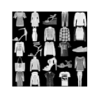
Experiment 1: Detect if a test set is from MNIST or fashion MNIST [34].
-
•
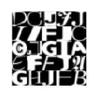
Experiment 2: Detect if a test set is from MNIST or non-MNIST [4].
-
•
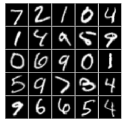
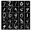
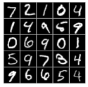
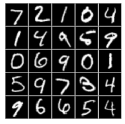
Experiment 3: Detect if a test set is from MNIST or synthetically-perturbed MNIST (see Table LABEL:tab:scenarios and Figure 1 for the description and visualization of the different dataset).
| Perturbation type, Value | |
|---|---|
| Case–1 | Rotation, |
| Case–2 | Shearing, |
| Case–3 | Width shift , Height shift, |
| Case–4 | Zooming, |
| Case–5 | Zooming, |
| Case–6 | Zooming, |
| Case–7 | Brightness, |
| Case–8 | Brightness, |
| Case–9 | Gaussian noise, |
The training data consists of black and white images: . In order to use Algorithm 2 in the current implementation, we had to downsample the image from to pixels. This is because Glow can not do dimensionality reduction, and our approach needs to compute . Inversion of high-dimensional matrices entails precision issues that can create invalid results; we are working on approximate matrix inversion to address this issue.
We solve OOD detection problem on test datasets of size . We repeated the experiment times; in 500 experiments, test data is from the same dataset as the training data), and in 500 experiments, test data is from a different dataset than the training data. It should be mentioned that we can not compare to the ddKS method used in Section IV-D because the data is too high-dimensional for the KS test.


We compared our approach to another Glow-based method called Typicality [24]. We trained our model with the same hyperparameters and settings as [24]. For a fair comparison, we trained and tested Typicality with both downsampled images. Table IV shows the AUROC for the experiments using different test set sizes . Our method has higher performance than Typicality method in all cases except Case–5. In particular, in Case–8, Typicality gives an AUROC less than (i.e., random guessing). This is because (as noted in the introduction) a likelihood-based approach, which does not learn alternative distribution, may encounter situations where the OOD test data has a high likelihood under the learned default model.
| MEC | Typicality | MEC | Typicality | MEC | Typicality | |
|---|---|---|---|---|---|---|
| fashion MNIST | ||||||
| not-MNIST | ||||||
| Case–1 | ||||||
| Case–2 | ||||||
| Case–3 | ||||||
| Case–4 | ||||||
| Case–5 | ||||||
| Case–6 | ||||||
| Case–7 | ||||||
| Case–8 | ||||||
| Case–9 | ||||||
VII Conclusion, Limitations, and Future work
We developed a method for OOD detection based on MDL for the case when the default distribution is known and when is unknown. In terms of application, the latter case is more likely to occur. We showed with experiments that our approach outperforms KS test for multivariate Gaussian and near-Gaussian OOD detection problems. We tested our approach on MNIST dataset and compared with another OOD detection method called Typicality. Our approach has higher performance in most of cases. It also does not give AUROC less than 0.5.
In this paper, we restricted the class of potential data models to only multivariate Gaussian distributions. Since the neural network transforms the default model into Gaussian, this is still powerful enough to detect subtle changes. However, if the test data is from distributions very different from the default distribution, it is unlikely that the transformed distribution will be close to Gaussian. The advantage of using MDL is that we can add any other model/coder into the framework as long as we account for complexity through MDL. In the future, we plan to expand our method with mixture of Gaussians and an extension of the histogram approach in one dimension to higher dimensions.
We also have numerical challenges with our current implementation because our method needs to compute covariance matrix and precision matrix . High-dimensional data means that these matrices are large and precision issue means that the inversion results may not be valid covariance/precision matrices. We will investigate fast, approximate matrix inversion algorithms (e.g., [3]) to solve this problem.
References
- Abolfazli et al. [2021a] Mojtaba Abolfazli, Anders Høst-Madsen, June Zhang, and Andras Bratincsak. Graph coding for model selection and anomaly detection in gaussian graphical models. In ISIT’2021, Melbourne, Australia, July 12-20, 2021, 2021a.
- Abolfazli et al. [2021b] Mojtaba Abolfazli, Anders Host-Madsen, June Zhang, and Andras Bratincsak. Graph compression with application to model selection. arXiv preprint arXiv:2110.00701, 2021b.
- Benzi and Tuma [2000] Michele Benzi and Miroslav Tuma. Orderings for factorized sparse approximate inverse preconditioners. SIAM Journal on Scientific Computing, 21(5):1851–1868, 2000.
- Bulatov [2011] Yaroslav Bulatov. Notmnist dataset. Google (Books/OCR), Tech. Rep.[Online]. Available: http://yaroslavvb. blogspot. it/2011/09/notmnist-dataset. html, 2, 2011.
- Chalapathy et al. [2018] Raghavendra Chalapathy, Edward Toth, and Sanjay Chawla. Group anomaly detection using deep generative models. In Joint European Conference on Machine Learning and Knowledge Discovery in Databases, pages 173–189. Springer, 2018.
- Chandola et al. [2009] Varun Chandola, Arindam Banerjee, and Vipin Kumar. Anomaly detection: A survey. ACM computing surveys (CSUR), 41(3):1–58, 2009.
- Corder and Foreman [2014] Gregory W Corder and Dale I Foreman. Nonparametric Statistics: A Step-by-Step Approach. John Wiley & Sons, 2014.
- Cover and Thomas [2006] Thomas.M. Cover and Joy.A. Thomas. Information Theory, 2nd Edition. John Wiley, 2006.
- Dempster [1972] A. P. Dempster. Covariance selection. Biometrics, 28(1):157–175, 1972. ISSN 0006341X, 15410420. URL http://www.jstor.org/stable/2528966.
- Deng [2012] Li Deng. The mnist database of handwritten digit images for machine learning research. IEEE Signal Processing Magazine, 29(6):141–142, 2012.
- Elias [1975] P. Elias. Universal codeword sets and representations of the integers. Information Theory, IEEE Transactions on, 21(2):194 – 203, mar 1975. ISSN 0018-9448. doi: 10.1109/TIT.1975.1055349.
- Fasano and Franceschini [1987] Giovanni Fasano and Alberto Franceschini. A multidimensional version of the kolmogorov–smirnov test. Monthly Notices of the Royal Astronomical Society, 225(1):155–170, 1987.
- Friedman et al. [2008] Jerome Friedman, Trevor Hastie, and Robert Tibshirani. Sparse inverse covariance estimation with the graphical lasso. Biostatistics, 9(3):432–441, 2008.
- Grunwald [2007] Peter D. Grunwald. The Minimum Description Length Principle. MIT Press, 2007.
- Hagen et al. [2021] Alex Hagen, Shane Jackson, James Kahn, Jan Strube, Isabel Haide, Karl Pazdernik, and Connor Hainje. Accelerated computation of a high dimensional kolmogorov-smirnov distance. arXiv preprint arXiv:2106.13706, 2021.
- HALL and HANNAN [1988] PETER HALL and E. J. HANNAN. On stochastic complexity and nonparametric density estimation. Biometrika, 75(4):705–714, 12 1988. ISSN 0006-3444. doi: 10.1093/biomet/75.4.705. URL https://doi.org/10.1093/biomet/75.4.705.
- Hastie et al. [2017] Trevor Hastie, Robert Tibshirani, and Jerome Friedman. The elements of statistical learning data mining, inference, and prediction, 2017.
- Høst-Madsen et al. [2019] Anders Høst-Madsen, Elyas Sabeti, and Chad Walton. Data discovery and anomaly detection using atypicality. IEEE Transactions on Information Theory, 65(9), September 2019.
- Kingma and Dhariwal [2018] Durk P Kingma and Prafulla Dhariwal. Glow: Generative flow with invertible 1x1 convolutions. Advances in neural information processing systems, 31, 2018.
- Lehmann et al. [1986] Erich Leo Lehmann, Joseph P Romano, and George Casella. Testing statistical hypotheses, volume 3. Springer, 1986.
- Li and Vitányi [2008] Ming Li and Paul Vitányi. An Introduction to Kolmogorov Complexity and Its Applications. Springer, fourth edition, 2008.
- Moulin and Veeravalli [2019] Pierre Moulin and Venugopal V. Veeravalli. Statistical Inference for Engineers and Data Scientists. Cambridge University Press, 2019.
- Muandet and Schölkopf [2013] Krikamol Muandet and Bernhard Schölkopf. One-class support measure machines for group anomaly detection. arXiv preprint arXiv:1303.0309, 2013.
- Nalisnick et al. [2019] Eric Nalisnick, Akihiro Matsukawa, Yee Whye Teh, and Balaji Lakshminarayanan. Detecting out-of-distribution inputs to deep generative models using typicality, 2019. URL https://arxiv.org/abs/1906.02994.
- Rabanser et al. [2019] Stephan Rabanser, Stephan Günnemann, and Zachary Lipton. Failing loudly: An empirical study of methods for detecting dataset shift. Advances in Neural Information Processing Systems, 32, 2019.
- Rissanen et al. [1992] J. Rissanen, T.P. Speed, and B. Yu. Density estimation by stochastic complexity. IEEE Transactions on Information Theory, 38(2):315–323, 1992. doi: 10.1109/18.119689.
- Rissanen [1978] Jorma Rissanen. Modeling by shortest data description. Automatica, pages 465–471, 1978.
- Rissanen [1983] Jorma Rissanen. A Universal Prior for Integers and Estimation by Minimum Description Length. The Annals of Statistics, 11(2):416 – 431, 1983. doi: 10.1214/aos/1176346150. URL https://doi.org/10.1214/aos/1176346150.
- Rissanen [1986] Jorma Rissanen. Stochastic Complexity and Modeling. The Annals of Statistics, 14(3):1080 – 1100, 1986. doi: 10.1214/aos/1176350051. URL https://doi.org/10.1214/aos/1176350051.
- Sabeti and Høst-Madsen [2019] Elyas Sabeti and Anders Høst-Madsen. Data discovery and anomaly detection using atypicality for real-valued data. Entropy, page 219, Feb. 2019. Available at https://doi.org/10.3390/e21030219.
- Serfling [2001] Robert J. Serfling. Approximation Theorems of Mathematical Statistics. Wiley-Interscience, 2001.
- Shamir [2006] G.I. Shamir. On the mdl principle for i.i.d. sources with large alphabets. Information Theory, IEEE Transactions on, 52(5):1939–1955, May 2006. ISSN 0018-9448. doi: 10.1109/TIT.2006.872846.
- Willems et al. [1995] F. M J Willems, Y.M. Shtarkov, and T.J. Tjalkens. The context-tree weighting method: basic properties. Information Theory, IEEE Transactions on, 41(3):653–664, 1995. ISSN 0018-9448. doi: 10.1109/18.382012.
- Xiao et al. [2017] Han Xiao, Kashif Rasul, and Roland Vollgraf. Fashion-mnist: a novel image dataset for benchmarking machine learning algorithms. arXiv preprint arXiv:1708.07747, 2017.
- Yamanishi and Fukushima [2018] Kenji Yamanishi and Shintaro Fukushima. Model change detection with the mdl principle. IEEE Transactions on Information Theory, 64(9):6115–6126, 2018.
- Yamanishi et al. [2021] Kenji Yamanishi, Linchuan Xu, Ryo Yuki, Shintaro Fukushima, and Chuan-hao Lin. Change sign detection with differential mdl change statistics and its applications to covid-19 pandemic analysis. Scientific Reports, 11(1):19795, 2021.
- Zhang et al. [2020] Yufeng Zhang, Wanwei Liu, Zhenbang Chen, Ji Wang, Zhiming Liu, Kenli Li, and Hongmei Wei. Towards out-of-distribution detection with divergence guarantee in deep generative models. arXiv preprint arXiv:2002.03328, 2020.