Hydrodynamics of a Discrete Conservation Law
Abstract
The Riemann problem for the discrete conservation law is classified using Whitham modulation theory, a quasi-continuum approximation, and numerical simulations. A surprisingly elaborate set of solutions to this simple discrete regularization of the inviscid Burgers’ equation is obtained. In addition to discrete analogues of well-known dispersive hydrodynamic solutions—rarefaction waves (RWs) and dispersive shock waves (DSWs)—additional unsteady solution families and finite time blow-up are observed. Two solution types exhibit no known conservative continuum correlates: (i) a counterpropagating DSW and RW solution separated by a symmetric, stationary shock and (ii) an unsteady shock emitting two counter-propagating periodic wavetrains with the same frequency connected to a partial DSW or a RW. Another class of solutions called traveling DSWs, (iii), consists of a partial DSW connected to a traveling wave comprised of a periodic wavetrain with a rapid transition to a constant. Portions of solutions (ii) and (iii) are interpreted as shock solutions of the Whitham modulation equations.
I Introduction
The hydrodynamics of the conservation law (inviscid Burgers’ equation)
| (1) |
with , is succinctly expressed by solutions of the Riemann problem that consists of Eq. (1) for subject to the initial condition
| (2) |
for . Solutions must be interpreted in a weak sense and depend intimately upon the regularization applied. For the viscous regularization in which equation (1) is modified to Burgers’ equation where , the weak solution of (1)—either a moving discontinuity (shock) or rarefaction wave (RW)—is uniquely determined by considering the strong vanishing viscosity limit of Burgers’ equation [1]. This results in the well-known Rankine-Hugoniot jump condition for the speed and Lax entropy condition of admissible shock solutions. Regularization by more complex viscous terms (nonlinear, higher order, and viscous-dispersive) generally results in the same weak solution [2]. An alternative dispersive regularization is the Korteweg-de Vries (KdV) equation . In this case, the zero dispersion limit converges weakly in the sense that it satisfies the KdV-Whitham modulation equations corresponding to averaged conservation laws [1, 3]. Gurevich and Pitaevskii recognized the physical importance of the asymptotic approximation obtained by considering small but nonzero and obtained the dispersive shock wave (DSW) solution of the KdV equation for (2) when as a self-similar solution of the KdV-Whitham modulation equations [4, 1]. They also observed that when , the KdV equation with small but nonzero is well-approximated by the same RW obtained by viscous regularization. Dispersive shock waves are unsteady, modulated nonlinear wavetrains connecting two distinct levels [5]. In contrast to viscous regularization, alternative dispersive regularizations can result in drastically different Riemann problem solution behavior in the small dispersion regime, particularly when higher order [6] or nonlocal [7] dispersive terms are considered. The multiscale dynamics of conservative nonlinear wave equations in the small dispersion regime are generally referred to as dispersive hydrodynamics [5].
In this paper, we study the dispersive hydrodynamics of the discrete regularization of Eq. (1)
| (3) |
by solving the Riemann problem
| (4) |
for (3) where . Equation (3) is the simplest centered differencing scheme for the hydrodynamic flux. As recognized in the early days of computational fluid dynamics by Von Neumann, and later clarified by Lax, differencing schemes like (3) introduce oscillations that require mitigation if one wishes to converge strongly to viscously regularized solutions that satisfy the conservation laws of fluid dynamics [8]. In this paper, we consider Eq. (3), subject to (4), in its own right, divorced from the aim of approximating solutions of Eq. (1). The semi-discrete equation (3) can be interpreted as the dispersive regularization
| (5) |
by introducing , into Eq. (3), where is the lattice spacing. Here, is the pseudo-differential operator for the centered discrete derivative and acts on a function in the variable via
| (6) |
Equation (5) is similar to Whitham type evolutionary equations [9, 10, 11] except that it is further constrained to be band-limited. For the lattice equation (3) at time , the support of the discrete-space Fourier transform of is due to the smallest length scale set by the lattice spacing, whereas the Fourier transform of quasi-continuum approximations is not generally compactly supported. As we will demonstrate, this fundamental property of lattice equations introduces new hydrodynamic solution features that do not appear within certain continuum limits of the model.
Equation (5) can be used to formally derive quasi-continuum approximations by using Padé approximants of for . For example, the (1,3) Padé approximant
| (7) |
leads to the Benjamin-Bona-Mahoney (BBM) equation absent the linear convective term [12]
| (8) |
This quasi-continuum approximation, inspired by the work of Rosenau on mass-spring chains [13, 14]—see also the discussion in [15]—is expected to faithfully represent the long-wavelength behavior of the lattice model (3). But it is no longer band-limited. In fact, outside of RWs and DSWs, the Riemann problem solutions we obtain for the lattice equation (3) bear no resemblance to the corresponding Riemann problem solutions of (8) obtained in [7]. Nevertheless, the quasi-continuum model (8) admits exact solitary and periodic traveling wave solutions that can be used to approximate corresponding solutions of the lattice model (3).
A particular feature of the band-limited lattice equation (3), and others with centered differences, is the existence of stationary, period two (binary) oscillation solutions
| (9) |
for any . Equation (3) was studied in [16] using extensive numerical simulations for certain types of odd initial data and binary oscillations were found to play an important role. Allowing for slow spatio-temporal modulations of this solution—, , , , —Turner and Rosales [16] obtained the modulation equations
| (10) |
Two important implications of the hydrodynamic-type equations (10) are: (i) the equations (10) are elliptic whenever and (ii) the existence of discontinuous, shock solutions satisfying Rankine-Hugoniot jump conditions. The ellipticity of (10) was shown to provide a route through modulated binary oscillations to blow up of solutions of (3).
While the topic of DSWs and dispersive hydrodynamics has been more extensively explored in the realm of continuum media [17, 5], as already implied by the above discussion, studies of the discrete realm have the potential to offer new and intriguing wave features. In addition, the motivation for such explorations has significantly increased on account of a diverse range of corresponding applications. A central topic is the study of granular crystals and associated nonlinear metamaterials [15], consisting typically of elastically interacting bead chains. There, a sequence of experimental efforts in simpler [18, 19], as well as in progressively more complex media, including dimers [20] and the more recent setup of hollow elliptic cylinders [21] have manifested the spontaneous emergence of DSWs under suitable loading conditions. However, this has not been the only setting where “effectively discrete” DSWs have experimentally emerged. Another example is in nonlinear optics where such structures have appeared in optical waveguide arrays [22]. Finally, and quite recently, yet another setup has emerged, that of tunable magnetic lattices [23] in which ultraslow shock waves can arise and be experimentally imaged.
Earlier interest in lattice shocks include the heyday of conservation laws and shock waves in the fifties and sixties when material scientists were interested in the compression of a solid by passage of a very strong shock wave through materials [24]. Early numerical studies (molecular dynamics simulations) depicted what we now call a lattice DSW in the material’s stress profile and recognized its unsteady character in a one-dimensional anharmonic chain [25]. This contradicted the basic assumption of steadiness underlying the Rankine-Hugoniot jump conditions and led to some controversy in the field. The DSW’s leading edge was then identified with a homoclinic traveling wave solution (solitary wave) of a continuum approximation in [26], later identified as a generic feature of DSWs in continuum media [4, 27]. The controversy continued for about 15 years until, in 1979, three-dimensional lattice simulations were shown to exhibit a transition from unsteady to steady shock fronts due to transverse strains [28]. It is worth noting that the same transition from one-dimensional, unsteady (dispersive) to multi-dimensional, steady (effectively viscous) shock propagation, was recently observed in a completely different, ultracold atomic superfluid [29].
| SS | Stationary shock |
|---|---|
| RW | Rarefaction wave |
| DSW | Dispersive shock wave |
| DSW+SS+RW | DSW + stationary shock + RW |
| TDSW | traveling DSW |
| Blow up | |
| US | Unsteady shock |
These works have motivated the present authors to revisit “lattice hydrodynamics” and the prototypical settings where DSW structures can arise in nonlinear dynamical lattices. Canonical examples of first order in time, quadratically nonlinear lattice nonlinear ordinary differential equations (ODEs) in a conservation law form were discussed extensively in the work of [16]. A subset of the present authors has recently revisited this class of models in [30] attempting to incorporate tools from Whitham modulation theory, bringing to bear both data-driven, as well as more theoretically-inspired quasi-continuum approaches to obtain an effective dimensional reduction, through an ODE description of the DSW states. Our aim here is to expand on this work, offering a more systematic classification of the possible solutions of such models by using Whitham modulation theory and, where appropriate, quasi-continuum approximation considerations supplemented by direct numerical simulations.
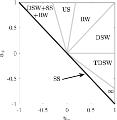
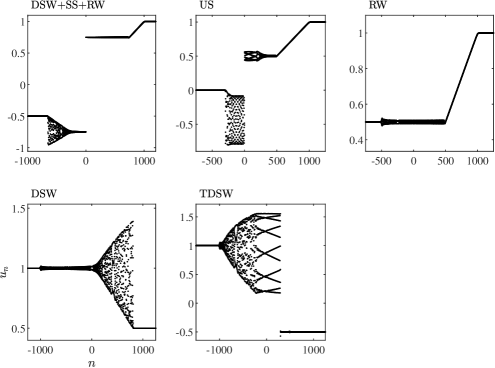
We select the scale invariant, representative nonlinear example (3) within the class of models of [16] and set up the corresponding discrete Riemann problem (4). Figure 1 depicts our phase diagram as a partitioning of the parameter space , and identifies seven distinct solution behaviors. Some of these, such as the possibility of a RW or a DSW as well as that of blow up are to a certain degree expected or have been argued to be present previously [16]. They are labeled RW, DSW, and in Fig. 1, respectively. However, there are choices of initial conditions that yield less common dynamical outputs, some of which are genuinely discrete in nature with labels in Fig. 1 identified parenthetically. These include, for instance, a stationary, symmetric shock on its own (SS) or separating a RW and a DSW (DSW+SS+RW). Another example is a traveling DSW (TDSW), which consists of a partial DSW connected to a heteroclinic periodic-to-equilibrium traveling wave. Arguably the most complex structure encountered is an unsteady shock evolving between two distinct traveling waves featuring the same temporal frequency (US). In what follows, we explain our partitioning of the phase diagram 1 into the regions pertaining to these different dynamical behaviors and we offer a set of tools that can be used to understand each one, as well as unveil some open directions for future exploration.
There exists a family of Riemann problems that can be considered in the discrete setting by modifying the value in (4). For example, Turner and Rosales set and [16]. We primarily focus on the data (4) in which resulting in the phase diagram of Fig. 1. While changing does not affect the observed solution phases, it does change the phase boundaries. We interpret this microscopic modification of the initial data impacting the macroscopic properties of solutions as an indication of non-uniqueness of the Riemann problem for the dispersive regularization (7).
It is important to distinguish our use of the term “shock” or “shock wave” from the classical notion of discontinuous weak solutions of inviscid Burgers’ equation (1). We identify four classes of shock solutions to the discrete equation (3) by prefacing each with a descriptor in Fig. 1. The simplest is the symmetric, stationary shock (SS) solution of the lattice
| (11) |
where . The other shock solutions can be understood as special solutions of the first-order, quasi-linear Whitham modulation equations corresponding to Eq. (3) that are described in Sec. III. The unsteady dispersive shock wave (DSW) is approximated by a nonlinear, periodic wavetrain modulated by a rarefaction wave solution of the Whitham modulation equations. Note that the DSW does not satisfy the Rankine-Hugoniot jump conditions of the Whitham modulation equations. On the other hand, the unsteady shock (US) is approximated by two periodic traveling waves that satisfy the jump conditions for the Whitham modulation equations. The traveling dispersive shock wave (TDSW) consists of both an unsteady partial DSW—approximated by a rarefaction solution of the Whitham modulation equations—and a steady traveling wave—approximated by a periodic traveling wave and a solitary wave that satisfy the jump conditions for the Whitham modulation equations. There is an important distinction between the traveling wave and US as discontinuous solutions of the Whitham modulation equations. The phase speeds of the two periodic traveling waves in the US solution differ from one another and from the shock speed, which is zero. On the other hand, the traveling wave solution consists of a single periodic traveling wave whose phase speed is the same as the shock speed. For clarity, we summarize the four distinct uses of the term “shock” in this paper:
-
1.
the stationary lattice shock (SS) (11);
-
2.
the unsteady dispersive shock wave (DSW) that is approximated by a rarefaction solution of the Whitham modulation equations;
-
3.
the unsteady shock (US) that is approximated by a discontinuous shock solution of the Whitham modulation equations;
-
4.
the traveling dispersive shock wave (TDSW) that is approximated by a shock-rarefaction solution of the Whitham modulation equations.
Our presentation will be structured as follows. In section II, we present the model equations, as well as the principal setup and notation for our study. In section III, we focus on the Whitham modulation equation formulation for the discrete problem. We discuss the corresponding conservation laws and how their averaging can provide information for the DSW features of our model. Section IV is dedicated to the systematic classification of our solutions in the different parametric regimes, accompanied by illustrative numerical computations of the different identified waveforms. In section V, we show how modification of the Riemann data (4) at a single site can lead to drastically different solution behaviors. Finally, in section VI, we summarize our findings and present our conclusions, as well as a number of open questions for further research into this budding theme.
II Model Equations
It will be beneficial to generalize Eq. (3) and consider the discrete scalar conservation law [16]
| (12) |
a discretization of the more general conservation law , where and the potential is assumed to be smooth with a convex function of its argument . Equation (12) possesses a Lagrangian and Hamiltonian structure [31], yet it is first order only, making its analysis slightly more convenient when compared to classical nonlinear oscillators, such as those of the Fermi-Pasta-Ulam-Tsingou (FPUT) type [32]. Besides serving as a prototype model for lattice DSWs, Eq. (12) is also of interest for applications, such as in the description of traffic flow [33]; for a discussion of relevant models and their continuum limits see also Ref. [16].
In this paper, we primarily focus on the potential
| (13) |
For this choice, the “mass”
and “energy”
when well-defined, are conserved in the infinite lattice and in a finite lattice with periodic boundary conditions. The linear dispersion relation for Eq. (12) is
| (14) |
for linearized wave solutions of the form , . Throughout the manuscript we consider the Riemann, step initial data (4). For numerical simulations, the infinite lattice is truncated by introducing (even) to represent the number of lattice sites. The corresponding spatial domain is and the simulation temporal domain is , where is a fixed constant independent of . We use free boundary conditions and in conjunction with the initial data Eq. (4), and we choose domain sizes large enough that interactions with the boundary are negligible. When investigating finite time blow up, we employ periodic conditions. This allows us to monitor if the rescaled quantities and are conserved (details in sec. IV.6). A variational integrator is used for simulations, see [31]. Simulations were also carried out with a Runge-Kutta method to check for consistency which yielded negligible differences on the time scales considered in this paper (for cases that did not involve blow up features). Due to the scaling symmetry , , for any nonzero of equation (12) subject to (13), we can set either or without loss of generality. Figure 1 shows a classification of the zoology of solutions that arise from the Riemann problem. They include rarefaction waves (RWs) for and , dispersive shock waves (DSWs) for and , solutions consisting of dispersive shock waves, stationary shocks and rarefaction waves (DSW + SS + RW) for and , solutions consisting of traveling dispersive shock waves (TDSW) for and , unsteady shocks (US) for and , and blow up () for and . The region boundaries are approximate. In sec. IV, we provide a detailed analysis for each of the five solution types just described, starting first with the simplest, and moving through them gradually in terms of their complexity according to the table in Fig. 1. We employ a number of tools for the study of these solutions, including direct numerical simulation, fixed-point iteration schemes, modulation theory, weak solutions, DSW fitting, and quasi-continuum modeling. The details of these approaches will be given in the sections they are employed, with the exception of modulation theory. This analysis is slightly more involved, and thus has a dedicated section. Our intention in presenting these tools is to leverage this specific, but interesting in its own right, example in order to utilize a variety of techniques that may be of broader relevance to applications in other Hamiltonian nonlinear dynamical lattices. It would be of particular interest to identify similar phenomena or/and to leverage the techniques utilized herein in other dispersive, nonlinear lattice models.
II.1 An alternative, integrable discretization
Prior to describing the solutions of Eq. (3) depicted in Fig. 1, we briefly comment on the alternative discretization
| (15) |
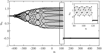
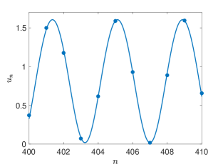
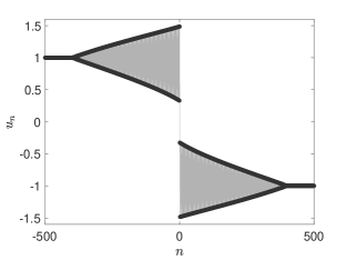
of Eq. (1) subject to (13). This equation was studied in [34, 35] where it was shown to exhibit DSWs and, for positive data, to be completely integrable by a transformation [36] to an equation related to the Toda lattice [37]. We have performed numerical simulations of Eq. (15) subject to the Riemann data (4) and observe DSWs when , RWs when and blow-up when and exhibit opposite signs. Examples of numerical simulations of DSWs and RWs that emerge from strictly positive initial Riemann data are shown in Fig. 2
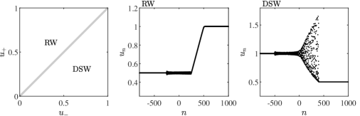
Of course, complete integrability confers a great deal of mathematical structure. Whitham modulation theory for the Toda lattice was developed in [38, 39, 40] while the inverse scattering transform for the Toda lattice with step-type initial data was developed in [41]; see also the recent discussion of Whitham theory applied to DSWs in the Toda lattice [42]. Collectively, these works support our numerical observation that, for positive Riemann data, Eq. (15) exhibits only RW and DSW solutions. These Riemann problem solution behaviors are to be contrasted with those depicted in Fig. 1. Although integrability of Eq. (15) is lost for sign indefinite initial data, the only dynamics we numerically observe are indicative of blow up. Thus, the discretization (3) we focus on in this paper, admits a wider variety of dynamics than the integrable alternative of (15).
III Whitham Theory
III.1 Modulation equations for a continuum system
In this section, we consider a continuum model system by introducing the interpolating function such that for all . This allows us to represent the advance-delay operator in the discrete system (12) as a pseudo-differential operator. The resulting continuum model is
| (16) |
Equation (16) can be written in the Hamiltonian form
| (17) |
where is the antisymmetric operator and is the Hamiltonian. Periodic solutions of (16) are of the form with phase and parameters (e.g., wavenumber, amplitude, mean). They satisfy
| (18) |
which is equivalent to the nonlinear advance-delay differential equation
| (19) |
The solution theory of such nonlocal equations is rather intricate but the existence of a three-parameter family of traveling waves has been establshed in [31] by variational techniques. Integrating (18) once with respect to
| (20) |
where is the phase speed and is a real constant. The pseudodifferential operator is then interpreted as a multiplier on the Fourier coefficients of ,
| (21) | ||||
| (22) |
Equation (16) possesses the two conserved quantities
| (23) | ||||
| (24) |
where the domain of integration is determined by the decay or periodicity of . We now seek the modulation equations for a periodic wave with the slowly varying ansatz
| (25) |
in which the leading order term is the periodic traveling wave solution satisfying (20) with vector of parameters that varies on the slow scales and while is 2-periodic in . We impose the generalized wavenumber and frequency relationships and along with their compatibility
| (26) |
Lemma 1.
The nonlocal operator acting on a modulated periodic function has the multiple scale expansion
| (27) | ||||
Proof.
The proof follows from the analyticity of . A detailed proof follows all of the ideas in [11]. ∎
We now average Eq. (16) and its higher order conserved densities by introducing the averaging operator
| (28) |
where is a local function of and its derivatives. If is a multiscale function of the form , then
| (29) |
by virtue of the fact that is periodic in so the period average of is zero. We use Lemma 1 to compute averages of, for example, for any with the Fourier series :x
| (30) | ||||
We now insert the multiple scales ansatz (25) into the two conservation laws associated with (16), and average. This procedure results in the system of conservation laws
| (31a) | ||||
| (31b) | ||||
| (31c) | ||||
In the vanishing amplitude limit, Eqs. (31a) and (31b) become the Hopf equation
| (32) |
for the mean , and the conservation of waves equation (31c) corresponds to linear wave modulation theory with frequency given by the linear dispersion relation (14).
The nonlinear modulation equations can alternatively be derived by employing Whitham’s other method of an averaged Lagrangian functional, see for instance [1, chapter 14] and [43] for symplectic PDEs, [44, 45, 46, 47] for an application to FPUT chains as the most prominent example of Hamiltonian lattices, and [30] for the discrete conservation law (12). In this setting, the modulation equations take the form
| (33a) | ||||
| (33b) | ||||
| (33c) | ||||
| This is a system of Hamiltonian PDEs with density variables , , and , which represent the wave mean, the nonlinear wave number, and a nonlocal auxiliary variable that might be regarded as a generalized wave momentum. Moreover, the equation of state describes the energy of a traveling wave and its partial derivatives provide the fluxes in (33). The energy is also conserved according to the extra conservation law | ||||
| (33d) | ||||
which is implied by (33) thanks to the chain rule. A closer look to the derivation of (33) in [30] reveals that (31a) and (31c) correspond to (33a) and (33b), respectively, while (31c) is the analogue to (33d). A complete understanding of (31) and (33) is currently out of reach because we are not able to characterize the analytical properties of the constitutive relations since these depend in a very implicit and not tractable way on the three-dimensional solution sets of the nonlinear advance-delay-differential equation (18). For instance, it is not even clear for which values of the parameters the Whitham system (33) is hyperbolic or genuinely nonlinear. For this reason we do not work with the full lattice modulation equations directly but combine different approximation procedures with a careful evaluation of numerical data.
III.2 Relation to the lattice dynamics
Although neither analytical nor numerical solutions to the nonlinear modulation systems (31) or (33) are available, we can extract important partial information from numerical simulations of initial value problems to (12). The key observation is that the lattice ODE as well as an implied energy equation represent discrete counterparts of local conservation laws and transform under the hyperbolic scaling of space and time into first order PDEs. To see this, we fix a window function that depends smoothly on the macroscopic variables , decays sufficiently fast, and has normalized integral. Using a shifted copy of , we are able to quantify the local moments of any microscopic observable near a fixed macroscopic point. For instance, the average
| (34) |
represents the mesoscopic space-time averages of near the macroscopic point .
Lemma 2.
Any bounded solution to (12) satisfies in the hyperbolic scaling limit the conservation laws
| (35a) | |||
| (35b) | |||
provided that these are interpreted in a distributional sense.
Proof.
We only give an informal derivation but mention that an alternative and more elegant framework is provided by the theory of Young measures. The latter can also be applied to non-smooth window functions and reveals that the mesoscopic averages can be expected to be independent of the particular choice for . Using the abbreviation , discrete integration by parts as well as the smoothness of we verify
and by similar computations we obtain
The asymptotic validity of (35a) is thus a direct consequence of the microscopic dynamics (12), the definition of the bracket in (34), and the hyperbolic scaling. The lattice ODE (12) implies with
another discrete conservation law (in which the time derivative of a density is balanced by the discrete divergence of a flux quantity), so the second claim (35a) can be justified along the same lines. ∎
There is an important difference between the conservation laws in (31) and (35). The PDEs in (31) (and likewise those in (33)) are derived under the hypothesis that the lattice solution can be approximated by a modulated traveling wave, see (25), and the closure relations involve the (unknown) profile functions for traveling lattice waves as well as averages with respect to the scalar phase variable . Numerical simulations with well-prepared initial data (e.g., the Riemann initial data (4)) indicate that the approximation assumption concerning the microscopic data is indeed satisfied but no rigorous proof is available, neither for the lattice (12) nor for FPUT chains with convex interaction potential. The only exceptions are the few completely integrable cases but the details are still complicated and involve special coordinates related to the Lax structure. In particular, even for the lattice of Eq. (15) and the Toda chain it is not easy to compute how the phase averages in the modulation equations depend on the traveling wave parameters.
The status of (35) is completely different. The two PDEs can be established under very mild assumptions (boundedness of lattice solutions) and by means of fundamental mathematical principles (such as integration by parts and compactness in the sense of Young measures). They reflect universal constraints for the macroscopic dynamics, do not require any a-priori knowledge on the fine structure of the microscopic oscillations, and hold for a large class of initial data (which might even be oscillatory or random). Moreover, the mesoscopic space-time averages can easily by extracted from numerical data. In the simplest case, we use a straightforward box counting with space-time windows of microscopic length (or macroscopic length ). Of course, (35) does not provide a complete set of macroscopic equations and without further information it is not clear whether or how the fluxes can be computed in a pointwise manner from the densities. The equations are nevertheless very useful since they allow us to derive and check partial information on the solution of the modulation equations from numerical data. In particular, in the context of modulated traveling waves, the PDEs (35a) and (35b) correspond to (31a) and (31b), respectively.
III.3 Self-similar solutions
The Whitham modulation equations (31) are a system of conservation laws that can be compactly expressed in the form
| (36) |
where the vectorial density and flux depend on the slowly varying parameters through integrals of the periodic orbit . Equation (36) can also be expressed in the form
| (37) |
provided the inverse is nonsingular. We will use solutions of the Whitham equations to approximate the long time dynamics of solutions to the Riemann problem (3), (4). Consequently, it is natural to consider the Riemann problem
| (38) |
for the Whitham equations (36) themselves. Rarefaction (simple) wave solutions and discontinuous shock solutions of the binary oscillation modulation system (10) were used in [16] to interpret various features of the numerical solutions. In this work, we will make use of rarefaction wave and discontinuous shock solutions of the more general Whitham modulation equations (31).
The invariance of the Riemann problem (36), (38) with respect to the hydrodynamic scaling , for real suggests seeking self-similar solutions in the form , . Equation (37) possesses rarefaction waves satisfying [48]
| (39) |
where and , provided the characteristic field is genuinely nonlinear . Since lie on the same, one-dimensional integral curve, they are constrained by two integral relations resulting from integration of the third order ODEs (39). Admissibility requires . The eigenvalues can be interpreted as speeds. For example, in the context of DSWs, the trailing edge speed is and the leading edge speed .
Another class of self-similar solutions are discontinuous shock solutions to the Whitham system (31)
| (40) |
where is the velocity of the shock solution that satisfies the Rankine-Hugoniot jump conditions
| (41) |
The brackets denote the jump in its argument evaluated on the left and right triple that parameterize distinct, steady periodic orbits .
For strictly hyperbolic, genuinely nonlinear Whitham modulation equations with negative linear dispersion (), classical DSW solutions connecting the two constant states are described by a rarefaction solution of (39) in which is the middle characteristic speed and , . The two constraints that result from integrating (39) determine the trailing edge wavenumber and speed as well as the leading edge amplitude and speed [5]. Therefore, a classical DSW corresponds to a rarefaction wave solution of the modulation equations, not a shock solution. For DSW construction, we will use the DSW fitting method, which leverages certain structural properties of the Whitham modulation equations under the assumptions of strict hyperbolicity and genuine nonlinearity in order to obtain , , and by integrating a scalar ODE [49, 5].
Whitham himself pondered the notion of discontinuous shock solutions to his eponymous equations [1]. But their utility was only recently discovered in [6] where shock solutions of the Whitham modulation equations for a fifth order KdV (KdV5) equation were deemed admissible if there exists a heteroclinic traveling wave solution connecting the corresponding left and right periodic orbits, each moving with the same speed as the shock. Such traveling wave solutions are possible in higher order equations such as KdV5. These Whitham shocks were used to solve the Riemann problem for KdV5 and, later, were investigated in the Kawahara equation [50]. In this paper, we will show that similar Whitham shocks emerge as the traveling wave portion of the TDSW solution in Fig. 1. We also provide analytical and numerical evidence of the existence of a new class of Whitham shocks, i.e., shock solutions of the Whitham modulation equations (31) whose corresponding left and right periodic orbits possess the same frequency but different speeds than one another and the shock itself (see US in Fig. 1).
III.4 Weakly nonlinear regime
In the previous sections, we derived the modulation equations supposing the existence of a family of nonlinear periodic solutions. In the case where no known explicit periodic solution is available, it is useful to approximate the periodic solution with a truncated cosine series. The approximation via the Poincaré-Lindstedt method utilizes an asymptotic expansion of both the profile of the periodic solution and its frequency in the small amplitude parameter . The approximate periodic solution and its frequency are given, for a generic potential by
| (42) | ||||
| (43) |
which maintain their asymptotic ordering so long as
| (44) |
i.e., for , neither nor are too small. Inserting (42), (43) into the modulation equations (31), we obtain the weakly nonlinear Whitham modulation equations in conservative form by retaining terms up to
| (45) | ||||
| (46) | ||||
| (47) |
In the case of the cubic potential (13), our focus here, the modulation equations are
| (48a) | ||||
| (48b) | ||||
| (48c) | ||||
Properties of the modulation equations can be elucidated by casting them in quasi-linear form , where
| (49) |
A perturbation calculation gives the eigenvalues of the flux matrix to
| (50a) | ||||
| (50b) | ||||
| (50c) | ||||
with the corresponding right eigenvectors
| (51a) | ||||
| (51b) | ||||
| (51c) | ||||
The quasilinear system is strictly hyperbolic if all of the eigenvalues are distinct, and real valued. To the order of the approximation given, the weakly nonlinear system is strictly hyperbolic provided , , and
| (52) |
When and , the eigenvalues are ordered . When , Eqs. (48a) and (48b) coincide with the Hopf equation for the mean and the remaining equation corresponds to the conservation of waves from linear wave modulation theory. When , Eq. (48c) is identically satisfied. While intuition might suggest that (48a) and (48b) are somehow related to the modulation equations for binary oscillations (10), in fact, the asymptotic derivation breaks down. For example, the period average of the weakly nonlinear solution (42) is no longer but rather so that the density in (48a) does not correspond to the density in (35a). When , one should discard Eq. (48) altogether in favor of the modulation equations for binary oscillations (10), which apply beyond the weakly nonlinear regime considered here.
IV Classification of Solutions
From now onwards, we focus solely on the discrete equation (3) (Eq. (12) subject to (13)). Figure 1 depicts seven qualitatively distinct solution families to the Riemann problem (3), (4) depending upon the parameters in the initial data. We now proceed to describe each of these solution families using a combination of numerical simulation, Whitham modulation theory, and quasi-continuum approximation. The straight line boundaries between each solution family in Fig. 1 are determined empirically (to two decimal digits accuracy) and some are explained by analytical considerations. By a possible reflection of the lattice and a rescaling of time, we can, without loss of generality, set either while varying or set while varying . Therefore, we can map out the phase diagram in the plane by traversing the top and right edges of the square .
The special case in which is trivial but the case in which is the stationary shock (SS) solution (11). Otherwise, the solutions exhibit more complexity, which we now explore. We start with the simplest case first, and then work toward the richest, most complex scenario.
IV.1 Rarefaction waves (RWs)
The simplest observed dynamical structure is the rarefaction wave shown as RW in Fig. 1. Empirically, we find that they form when and . The bifurcation at will be described in section IV.5. The leading order RW behavior is given by the self similar solution ()
| (53) |
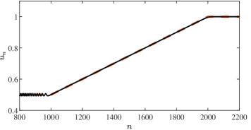
of the dispersionless equation (32). A favorable comparison of this profile with a numerical simulation is shown in Fig. 3. Because the data is expansive, the effect of dispersion manifests at higher order where a small amplitude, dispersive wavetrain is emitted from the lower, left edge of the RW.
The slowest (most negative) group velocity is , which corresponds to an inflection point of the linear dispersion relation (14). Consequently, the leftmost edge of these small amplitude waves is expected to have an Airy profile whose decay estimate is proportional to , similar to the Fourier analysis carried out for linear FPUT chains [51]. The details of the linear wavetrain accompanying RWs and DSWs for the BBM equation were studied in [7]. We follow a similar procedure by linearizing about the left initial state to obtain
| (54) |
The initial data (4) then becomes
| (55) |
whose discrete-space Fourier transform is the distribution
| (56) |
where is the Dirac delta. To approximate the nonlinear equation (3) by the linear equation (54), one could seek solutions in which . Alternatively, we follow [7] and consider scale separation in which the highest frequency components of (56) are assumed to separate from the RW so that the initial data becomes
| (57) |
for some that is sufficiently far from the zero dispersion points, . Then, the solution of the linear equation (54) can be determined by taking the discrete-space Fourier transform . The solution of Eq. (54) subject to (57) is
| (58) |
Quantitative information regarding the solution can be determined asymptotically for with fixed using the method of stationary phase [1]. The leading order behavior is determined by analyzing the integral (58) near the stationary points, where . Stationary points are therefore given by where
| (59) |
for . The leading order behavior in the vicinity of the stationary points is determined by expanding the integrand in (58) about the stationary points . When and , the leading order behavior is
| (60) |
The profile (60) is compared with numerical simulations of the initial value problem in Fig. 4 on the interval at a final simulation time of . The interval is chosen so that , i.e., the truncation parameter and we avoid the degenerate stationary points . We observe that the linear profile (60) is in good agreement with the numerical simulation. However, for larger initial jumps, the linear wave begins to deviate from the simulation. This may be attributed to the emergence of stronger nonlinear effects not captured by the leading order asymptotics which require a larger truncation parameter .
To investigate the leftmost edge of the linear wave emitted from the RW, we modify our previous analysis and expand the phase in the integral (58) about the inflection point of the linear dispersion relation
| (61) |
The expansion (61) is inserted into the integral (58). A calculation reveals that the leading order asymptotics in the vicinity of the ray are given by
| (62) |
where is the Airy function The Airy profile (62) favorably compares with the two Riemann problem simulations depicted in Fig. 5, even for large .
It is worth contrasting the observed RW dynamics with those of the quasi-continuum approximation in the BBM equation (8) that was studied in [7]. Qualitatively, the dynamics exhibited by the two models in overlapping regimes of the plane of Riemann data are very similar. Both equations exhibit large-scale dynamics that are well-approximated by the self-similar solution (53) and its analogue for the BBM equation. The details of the short-scale, emitted dispersive wavetrains are quantitatively different but, since both equations admit non-convex linear dispersion relations, they both exhibit Airy profiles with amplitude decay proportional to .
The long-time dynamics produced by the lattice model (3) significantly differs from those generated by its quasi-continuum BBM counterpart (8) when either equation is strongly influenced by small scale effects. The actual Riemann problems for the BBM equation studied in [7] were -smoothed, monotone transitions between and , a feature which introduces an external length scale characterizing the width of the initial transition. When this width is larger than the oscillatory length scale (or in Eq. (8)), the BBM equation exhibits a RW for all . As shown in Fig. 1, RW generation on the lattice is limited to the region , , with short-scale oscillatory dynamics occurring when , . When the BBM initial transition width is sufficiently small, RW generation can be accompanied by the spontaneous generation of solitary waves and/or an expansion shock, features not observed in the lattice model.
IV.2 Dispersive shock waves (DSWs)
For and the data is compressive and results in an expanding, modulated oscillatory wave train between the states and . This structure is called a dispersive shock wave; see the panel labeled DSW in Fig. 1. In [30], DSWs were studied in Eq. (35) with and , using numerical simulations and a dimension reduction approach. In the following, we study DSWs in the system (3) as the step value varies using two semi-analytical approaches, DSW fitting and a continuum model.
IV.2.1 Approximation of the DSW harmonic and soliton edge speeds via DSW fitting
In this section, we outline the method for fitting the macroscopic DSW properties (edge speeds, amplitudes, and wavenumbers) by applying the fitting method first introduced by El [49]; see also [5]. This method was originally developed and justified for continuum PDEs where it has been extensively applied. Since it only requires knowledge of the linear dispersion relation and the solitary wave amplitude-speed relation, it is straightforward to extend the method to the semi-discrete lattice equation (12).
An example DSW from a numerical simulation of the Riemann problem with and is shown in Fig. 6. The DSW is comprised of a modulated, nonlinear wavetrain that terminates in two distinct limits: vanishing amplitude (called the harmonic edge) and vanishing wavenumber (called the soliton edge). The modulation solution describing the DSW is the rarefaction solution (39) of the Whitham modulation equations (31) with , . The harmonic edge wavenumber and the soliton edge amplitude , as well as their corresponding edge speeds and are determined by integrating the ODE (39), thus relating these macroscopic DSW properties to the initial data . In numerical simulations, the amplitude of the DSW does not vanish exactly at the harmonic edge, so we define the location of the trailing edge by the intersection of the oscillatory envelope curves shown in Fig. 6.
Although the DSW modulation is determined, in principle, by the aforementioned rarefaction solution of the Whitham modulation equations (assuming strict hyperbolicity and genuine nonlinearity of the second characteristic field), we do not have explicit expressions relating the integrals in (31) to the periodic orbit’s parameters . An alternative technique that allows one to obtain the DSW’s edge properties is the DSW fitting method [5]. This method assumes the existence of the rarefaction solution. For the sake of completeness, we will carry out the DSW fitting procedure for a generic potential . The wavenumber of the DSW at the harmonic edge can be determined by solving the initial value problem
| (63) |
where is the linear dispersion relation (14). This ODE can be integrated by separation of variables to obtain
| (64) |
The wavenumber at the DSW harmonic edge is . The velocity of the harmonic edge is given by evaluating the linear group velocity at
| (65) |
The velocity of the DSW at the soliton edge is calculated in a similar way. We begin by introducing the conjugate variables , where acts as a soliton amplitude parameter. The velocity of the DSW soliton edge is deduced by evaluating the solitary wave dispersion relation , where we find by solving the initial value problem
| (66) |
Integration results in
| (67) |
and the soliton edge conjugate wavenumber . The soliton edge velocity of the discrete DSW is given by
| (68) |
Comparisons with numerical simulations of the Riemann problem are given in Fig. 7 with the potential and the initial data normalized so that . To estimate the velocity of the leading edge, we track the position of the right-most lattice site that is above the far-field initial data at the integer valued times in our numerical simulation. This time series data is fit with a line whose slope is the approximate velocity of the soliton edge of the DSW. To estimate the harmonic edge velocity, we produce a linear fit of the modulated wavetrain amplitude near the location of the harmonic edge, which is found by extracting peaks of the solution at output times. The intersection of this linear approximation with the constant level is the approximate location of the DSW harmonic edge. The time interval of our numerical computations varies depending on . For instance, when we take , we approximate the solution at , while taking requires the longer time for the solution to asymptotically develop. Upon varying , we observe good agreement between the predictions of DSW fitting for the DSW harmonic and soliton edge velocities and numerical simulations for , while the predictions begin to deviate from what is observed in numerical simulations below this threshold. The DSW fitting method is subject to the convexity conditions
| (69) |
A direct calculation for the potential demonstrates that these convexity conditions are indeed satisfied. The numerical results suggest that the DSW fitting method provides an adequate approximate prediction of the discrete DSW edge properties.
The harmonic edge of the DSW is accompanied by linear radiation much like the left edge of the RW in the previous section. To describe this, we apply the same approach as in Sec. IV.1 to approximating the small amplitude linear waves that emanate from the DSW’s harmonic edge. The only change is that, for the DSW, in Eq. (55). A comparison is shown in Fig. 8.
IV.2.2 Approximations of the leading edge amplitude via a quasi-continuum model
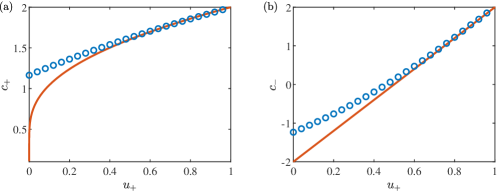
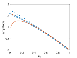
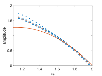
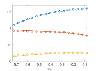
In this subsection, we go a bit deeper into the description of the solitary wave at the soliton edge of the DSW. Like in the previous subsection, for (where is fixed), we numerically solve the Riemann problem, generate a DSW and extract the amplitude of the soliton edge, and its speed. This is done by inspecting the time series of a node sufficiently far from the center of the lattice (we chose , in which case we have observed the leading edge is developed) and simply computing the amplitude as . The speed is estimated by computing where and are the time values where and attain their maxima. The blue open circles in Fig. 9(a) show the amplitude of the DSW soliton edge as a function of . Since for each value of , we compute both the speed and amplitude , we also show a parametric plot of parameterized by in Fig. 9(b).
To confirm that the DSW soliton edge is indeed described by a solitary wave, we compute a numerical solitary wave solution of the lattice equation (12) by using a fixed-point iteration scheme [31] to solve the advance delay equation
| (70) |
which is a rescaled copy of (18) and obtained by substituting
| (71) |
into Eq. (12). While we are free to select values of and when solving Eq. (70), we select combinations of them according to the relationship extracted from the DSW soliton edge (i.e., the blue circles in Fig. 9(a)). Upon convergence of the scheme, we compute the amplitude of the resulting solitary wave, which is the maximum of the wave minus the background . The amplitudes of the solitary waves are shown as the solid red dots in Fig. 9(a,b). Note that these red dots fall almost exactly within the blue circles, indicating that the soliton edge of the DSW is indeed well-approximated by a solitary wave solution of the lattice equation.
We can obtain an analytical approximation of discrete solitary waves by considering the BBM quasi-continuum approximation (8) of the lattice dynamics (3). Entering the moving frame and integrating once, this PDE becomes the second order ODE
| (72) |
where is an arbitrary integration constant. This ODE can be solved using quadrature [52]. In particular, the solitary wave with tails decaying to the background state has the form
| (73) |
which assumes . Note the maximum speed of linear waves on a background is , implying the solitary waves travel faster than all linear waves, as expected. In Eq. (73), and can be chosen independently of each other but we once again select combinations of them according to the relationship extracting from the DSW soliton edge (the blue circles in Fig. 9(a)). The solid blue dots of Figure 9(a) show the quasi-continuum prediction of the amplitude , where it is seen that the approximation becomes better as the jump height decreases (i.e., as ). The quasi-continuum prediction of the amplitude is only semi-analytical as it relies on the numerically obtained relationship of and from the DSW soliton edge data. An analytical prediction can be derived by using the DSW soliton edge speed in Eq. (68) of the previous subsection, which allows us to express the amplitude, , of the DSW soliton edge in terms of just (or ):
| (74) |
See the solid red line of Fig. 9(a,b) for a plot of this formula.
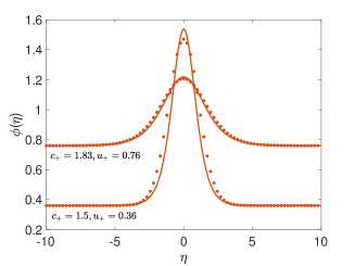
Finally, the solitary wave profile given by Eq. (73) matches the numerically computed solitary wave solution of Eq. (70) quite well, especially for longer wavelength solutions. See Fig. 9(c) for a comparison of the actual solitary wave (solid red dots) and quasi-continuum approximation (solid red line) for two example parameter sets.
(a)
 (b)
(b)
 (c)
(c)
Because the quasi-continuum approximation of DSWs here and in [30] performs well, we briefly contrast the Riemann problems that result in DSWs for the lattice (3) and BBM (8) equations. The DSW fitting technique was applied to the BBM Riemann problem in [7]. In order to compare our results for the lattice with DSWs in the BBM equation (8), we consider the initial transition occurring between and for . At the DSW harmonic edge, the characteristic wavenumber and speed for BBM agree to with the expansions and for the lattice. Similarly, at the DSW soliton edge, the conjugate wavenumber and speed agree to with the lattice: and . The DSW’s soliton edge amplitude in BBM is whereas the prediction (74) for the lattice expands as . Note that to leading order, these predictions agree with the DSW edge characteristics of the KdV equation for , , . This is expected because BBM and KdV are asymptotically equivalent to leading order in the weakly nonlinear, long wavelength regime.
In summary, the quasi-continuum approximation of lattice DSWs by DSWs in the BBM equation performs well for small initial jumps when the oscillation wavelengths are much larger than the lattice spacing. The agreement to in the DSW properties is expected and, in fact, is a statement of universality of the KdV equation as a weakly nonlinear, long wavelength model of dispersive hydrodynamics [5]. For sufficiently large , the BBM DSW develops two-phase modulations near the trailing edge [7]. In contrast, for , the lattice DSW bifurcates into a partial DSW connected to a traveling wave called a TDSW or exhibits blow up that we will describe in Secs. IV.4 and IV.6, respectively.
IV.3 Dispersive shock wave + stationary shock + rarefaction (DSW+SS+RW)
In this section we investigate the case where the initial step generates two unsteady waves: a leftward moving DSW and a right moving RW. At the origin, there is a stationary shock (SS) joining symmetric states at the level . A numerically computed example is depicted in Fig. 10. This class of solution is empirically found for and . As will be shown, the bifurcation at occurs when the DSW’s harmonic edge exhibits zero velocity.
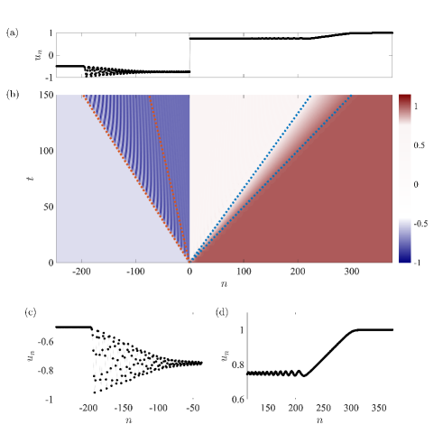
The numerical simulation shown in Fig. 10 suggests that the solution can be approximated for large as:
| (75) |
The velocities give the motion of the DSW’s soliton and harmonic edges, respectively. Across all of the simulations performed, we found the following relation for the intermediate, symmetric states to hold to very high precision
| (76) |
This relation implies that the DSW and RW have the same jump height, albeit with opposite polarities. We have been unable to mathematically justify this formula. However, as we show in section V, the value of the intermediate state depends strongly on particular details of the initial data. If the value of is changed, then the intermediate value differs from (76).
Utilizing the formula (76), we can completely determine the velocities that divide the approximate solution (75) into different wave patterns. To determine the DSW edge velocities, we use Eqs. (65) and (68), which were derived under the assumption that . In the case of the solution (75), the left () and right () states are both negative. Since the governing equation (3) is invariant under the transformation , the DSW velocities are mapped as follows
| (77) |
Then, using (76), we find
| (78) |
Figure 10(b) shows good agreement between the predicted velocities of the approximate solution (75) and a numerical simulation when , .
The DSW remains detached from the stationary shock (SS) so long as the harmonic edge velocity remains negative. From Eq. (78), we predict that the DSW is no longer detached from the SS when , which, for , occurs when . As noted earlier, the bifurcation from the DSW + SS + RW to the US case is empirically identified as occurring when . As shown in Fig. 10(b), this small discrepancy in the bifurcation value can be explained by the deviation of the computed DSW harmonic edge velocity from the DSW fitting prediction (65).
IV.4 Traveling dispersive shock wave (TDSW)
In this section, we consider the case where a partial DSW connects the level behind, , to a periodic-to-equilibrium traveling wave solution to the level ahead . Although we do not directly compute it as a traveling wave solution of the discrete equation, it is interpreted as a heteroclinic connection between a periodic orbit with the constant level ahead based on an analysis of the numerical simulations of the Riemann problem. Such heteroclinic solutions of continuum equations with higher (fifth) order dispersion were studied in [6, 50] and were associated with so-called traveling dispersive shock waves (TDSWs) that emerge from an associated Riemann problem.
For and , numerical simulations show a qualitatively similar solution pattern to that depicted in Fig. 11 in which begins on the left with the value . It then progresses into an oscillatory wavetrain with increasing amplitude that resembles the leftmost portion of a DSW, called a partial DSW, that is then connected to a periodic traveling wave. The periodic traveling wave is connected to the constant state ahead via an abrupt transition that moves with the same speed. Collectively, this partial DSW and traveling wave is referred to as the traveling DSW.
The TDSW solution studied here is the discrete analogue of the TDSW studied for the KdV5 equation [6]. The terminology traveling dispersive shock wave unites the unsteady component of the partial DSW and the steady traveling wave component (a heteroclinic periodic-to-equilibrium solution) to which it is attached in this non-classical DSW. Consequently, the entire TDSW structure is unsteady.
IV.4.1 Approximation of the traveling wave via the quasi-continuum model
One can describe the periodic portion of the TW (see e.g. the interval of Fig. 11) using the continuum reduction presented in section IV.2.2. In particular, there is a three-parameter family of traveling wave solutions of the quasi-continuum BBM Eq. (8), given by
| (79) |
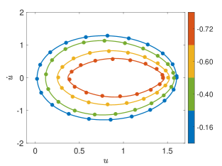
We treat as fitting parameters. After a sufficiently long time, the traveling wave in the numerical simulation forms, as in Fig. 11. We then isolate a small interval of that traveling wave, which is then fit to Eq. (79). Figure 12(a) shows a comparison of the actual lattice dynamics at (blue markers) and quasi-continuum approximation (blue lines) with the step values and . Figure 12(b) shows the trajectory in the phase plane (two outermost lobes) and (two innermost lobes) for various values of for the actual lattice dynamics (markers) and quasi-continuum approximation (lines). We show the phase plane for different values of since the location of the traveling wave within the lattice is moving. The agreement is quite good throughout the interval of existence for these structures, but is best when the jump height is smallest (compare the blue and red trajectory of Figure 12(b)). The comparison of the frequency, amplitude, and mean parameters is shown in Figure 12(c). These are computed via the following formulas with fixed. For the lattice index is fixed to , for the index is and for the index is . The frequency is , where is the period (computed as the peak-to-peak time of the trajectory); the mean is
where is the time interval of one oscillation period. For the computations shown here, it is . The amplitude is
Once the best-fit values of are obtained, the wave parameters can be computed directly from Eq. (79) as
where and are the complete elliptic integrals of the first and second kind, respectively. We note that while Eq. (8) is able to describe the local periodic traveling wave dynamics of the TDSW structure, it does not admit solutions resembling the entire TDSW structure since heteroclinic periodic-equilibrium solutions do not exist for the planar ODE (72). Such a description may be possible by using the (1,5) Padé approximant instead of the (1,3) approximant in (7) to arrive at the 5th order model
Similar models have been shown to admit such solutions [6]. While this is an interesting topic for further study, we will not pursue the identification of such a heteroclinic orbit further herein.
(a)
|
(b)
|
(c)
|
IV.4.2 Modulation solution of the weakly nonlinear Whitham modulation equations
In order to obtain the form of an approximate modulation solution of the Whitham equations (31) that describes the TDSW, we appeal to the structure of the TDSW evident in Fig. 11. An oscillatory wavetrain emerges from the left level with increasing amplitude that saturates at a periodic traveling wave. The traveling wave then abruptly transitions to the right level . Guided by previous work on the traveling dispersive shock wave (TDSW) solutions of a fifth-order Korteweg-de Vries equation [6], we make the self-similar modulation ansatz ()
| (80) |
for Eq. (37) where is the middle characteristic velocity. Additionally, the constant states are
| (81) |
and is the rarefaction solution (integral curve) of Eq. (39) for the second characteristic field that continuously connects the harmonic edge state and the periodic traveling wave state of the TDSW. The discontinuity from to satisfies the jump conditions (41) for the Whitham modulation equations where is simultaneously the phase speed of the periodic traveling wave with parameters , the shock speed, and the phase speed of the solitary wave with parameters , i.e., it represents the TW component of the TDSW solution. The modulation solution (80) corresponds to a rarefaction-shock solution of the Whitham modulation equations.
The five parameters in the modulation solution (80) could, in principle, be obtained by solving the full Whitham modulation equations (31), but we lack explicit periodic traveling wave solutions. Instead, we approximate the modulation solution (80) in the weakly nonlinear regime by solving Eqs. (48).
A general feature of Whitham modulation systems in the weakly nonlinear regime is the mean induced by the finite amplitude modulated wavetrain [1]. Absent mean changes due to initial/boundary data, the third order weakly nonlinear modulation system (48) can be simplified, with the same order of accuracy, to a second order modulation system. The procedure to do so is as follows. The induced mean is represented by the ansatz
| (82) |
where is a constant background. This introduces the induced mean coefficient that gives rise to an effective nonlinear frequency shift by inserting (82) into Eq. (43) and expanding as
| (83) |
With this effective nonlinear frequency shift, weakly nonlinear wave modulations are generically described by the simplified system [1]
| (84a) | ||||
| (84b) | ||||
provided
| (85) |
Note that the additional coupling term involving and its derivatives contribute at higher order in . The induced mean coefficient in Eq. (85) is determined by compatibility of averaged mean, energy conservation laws (48a), (48b) with the induced-mean modulation system (84), which asymptotically satisfies for any differentiable , in particular .
Under the assumption of induced mean variation, we can analytically obtain the rarefaction solution in (80) by solving Eq. (84) for a RW and then inserting it into Eq. (82). For this, we express the induced-mean modulation system in Riemann invariant form
| (86) |
where
| (87) |
The restriction to positive mean and wavenumber is due to the fact that we have selected the positive square root in (87). The characteristic velocities are
| (88) |
so that and in Eq. (50).
We can now solve for in (80) by setting and taking the fast RW solution of Eq. (86) that satisfies and . The constant slow Riemann invariant implies
| (89a) | |||
| and the assumption of induced mean implies | |||
| (89b) | |||
| The RW profile is obtained by inverting for and subject to the constraint | |||
| (89c) | |||
| Equations (89a) and (89b) are two conditions on the four unknown solution parameters . The other two conditions are obtained from the jump conditions (41). | |||
The sharp transition from the periodic traveling wave to the solitary wave ahead is achieved by a shock solution of the Whitham modulation equations. We obtain the jump conditions from the conservation laws (31a) and (31b) by assuming that the periodic traveling wave is in the weakly nonlinear regime (42) and the level ahead is a solitary wave where , both with the same phase speed :
| (89d) | ||||
| (89e) |
The jump condition from the conservation of waves equation (31c) is satisfied because for the solitary wave and for the periodic traveling wave
| (89f) |
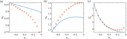
Solving for and from (89a) and (89b), then inserting them into (89d), (89e) and using the phase velocity (89f) determines two nonlinear equations for and . We solve these equations numerically using standard root finding methods to obtain all the parameters of the shock-rarefaction modulation solution (80) and compare it with numerical simulation in Figs. 13 and 14. We observe in the figures that near the onset of the TDSW, the solution’s mean, amplitude and frequency are accurately captured by the above theory. On the other hand, as the amplitude of the solution increases, the approximation loses quantitative efficacy. Nevertheless, the qualitative trend of the solution’s properties are captured by the above analysis.
IV.5 Unsteady Shock (US)
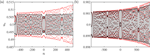
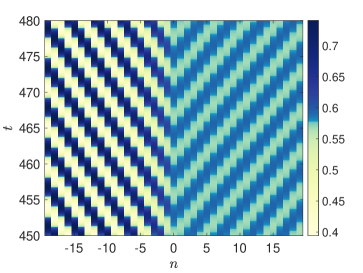
In section IV.3, we found that for and , a stationary shock separated two counterpropagating waves, one a DSW, the other a RW. When , the DSW no longer separates from the stationary shock. Instead, the DSW+SS+RW is numerically observed to bifurcate into the unsteady generation of counterpropagating periodic waves that we term an unsteady shock (US) for . When exceeds , the US bifurcates into a RW, described in section IV.1. We now investigate the US.
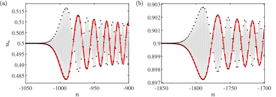
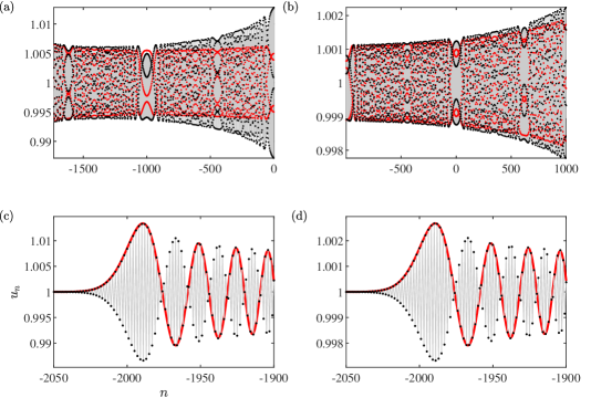
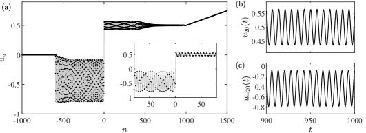
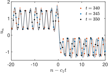
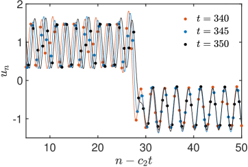
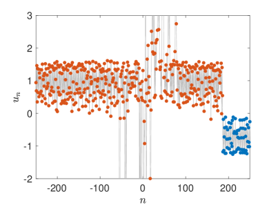
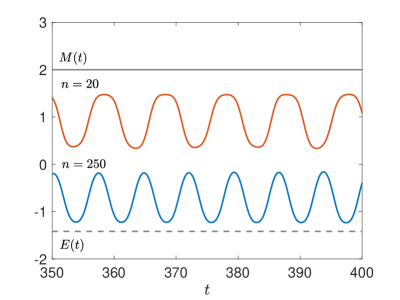
A plot of the solution for and is given in Figure 15. Two distinct counterpropagating periodic waves traveling with speed emerge from the origin that then transition to the constant level behind through a partial DSW and to ahead via a partial DSW and a RW. While the velocities are distinct, Figure 15(b) depicting the time series indicates that the two periodic waves have approximately the same temporal frequency, which we confirm below numerically to high precision.
(a)

|
(b)
|
(c)
|
(d)

|
IV.5.1 Poincaré description
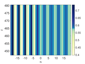
A spatio-temporal intensity plot of the US with near is shown in Fig. 16(a). The counterpropagating traveling waves can clearly be identified. While the underlying wave parameters of the left- and right-moving waves will generally be different, they do share the same frequency. Thus, the dynamics correspond to a time-periodic solution. Indeed, inspection of Fig. 16(c) confirms this, which shows the same intensity plot as panel (a), but with the solution sampled every time units, where is the period of oscillation. This is the Poincaré map of the dynamics. With this sampling size, the solution appears to be constant, suggesting that the waveform is genuinely time-periodic. To demonstrate this further, we simulated the equations of motion on a small lattice with boundary conditions given by the periodic solution, i.e., the left boundary is given by and the right boundary is given by . The dynamics upon initialization with the periodic solution are shown in Fig. 16(b), which can be hardly distinguished from the dynamics in (a). The evolution remains periodic, as can be inferred from Fig. 16(d), which are the dynamics sampled every seconds. An avenue for potential further study, prompted by these findings, is the seeking of exact time-periodic solutions of the model and their corresponding Floquet analysis.
IV.5.2 Approximation of traveling waves via quasi-continuum model
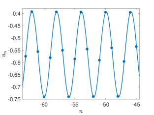
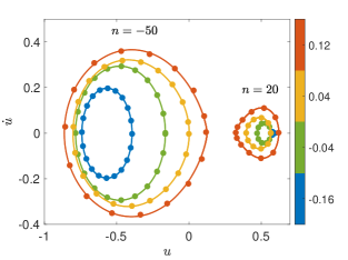
If considering the left-moving and right-moving waves as separate entities, we can once again apply the quasi-continuum reduction to describe the traveling wave using formula Eq. (79). A comparison of the spatial profile of the left wave moving wave with at time is shown in Fig. 17(a). The phase plane for the left-moving waves (left lobes) and right-moving waves (right lobes) is shown in Fig. 17(b) in markers, with corresponding quasi-continuum approximations shown as solid lines. Like before, the reduction is best for smaller step heights (compare the blue and red orbits in panel (b)). A comparison of the mean, amplitude and frequency of the simulation and quasi-continuum approximation as a function of is shown in panel (c) for both the left- and right-moving waves. We can observe that the approximation provides a very adequate description of the relevant traveling patterns.
(a)
|
(b)
|
(c)
|
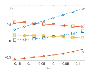
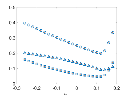
IV.5.3 Jump Conditions
Figure 16 shows two counterpropagating periodic traveling waves with a rapid transition between them in the vicinity of . This motivates the hypothesis that these two waves satisfy the jump conditions obtained from the Whitham modulation system’s conservation laws. We denote the periodic traveling waves by for the left () and right () periodic waves, respectively. For a discontinuous, shock solution of the Whitham system at the origin, the corresponding jump conditions are Eq. (41)
| (90a) | ||||
| (90b) | ||||
| (90c) | ||||
where is the unit shift operator . To check if these jump conditions are indeed satisfied, we approximate the above averages using the numerical simulations. In particular, we let the structure come close to a periodic state (as in Fig. 16) and extract one period of motion at a particular node . Let be the period of node and let be the corresponding time interval from . We then make the following approximations
| (91a) | ||||
| (91b) | ||||
for (we set in what follows). The first jump condition, Eq. (90a), is checked by comparing to , while the second jump condition Eq. (90b) is checked by comparing with . The third jump condition is simply the difference in the frequency, which we estimate via and . Figure 18 shows a plot of (open blue circles), (open blue squares) and (open blue triangles), while the red dots show the corresponding quantities for . Notice that each red point falls nicely into an open blue marker, indicating that the jump conditions are, up to some small numerical error, satisfied. The maximum residual over the interval of values tested for the first jump condition was , whereas the maximum residual for the second condition was and the maximum residual for the third was .
The numerical evidence is a compelling indication that the US can be interpreted as a shock solution of the Whitham modulation equations. While shock solutions of the Whitham equations have been constructed previously [6, 50], their admissibility requires the existence of traveling wave solutions of the corresponding continuum PDE in which the phase velocities and shock velocity all coincide. In the present case of the US for the lattice equation (3), all three of these velocities differ but the frequencies are the same. This suggests a new class of admissible shock solutions to the Whitham equations corresponding to time-periodic solutions of the lattice equation, an intriguing possibility for future work.
We also note the similarity between the US and defect solutions of reaction-diffusion equations [53]. Because the waves in the US are in-phase (see Fig. 16), it most closely resembles a target pattern with a source from which waves are emanating, in the language of [53]. The target pattern exhibits a Hopf bifurcation of the background state and a specific transition of the eigenvalues associated with the linearized operator about the background state. It would be interesting to explore potential connections between the underlying diffusive regularization of the target pattern and the dispersive regularization of the US studied here.
IV.6 Blow up
(a)
|
(b)
|
(c)
|
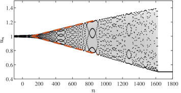
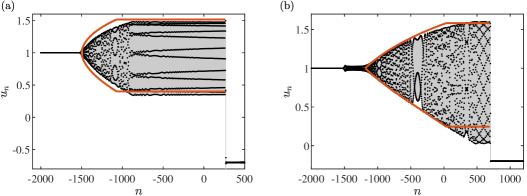
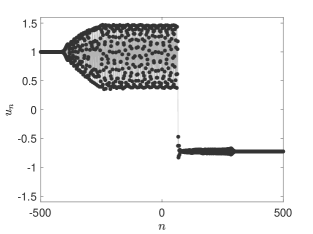
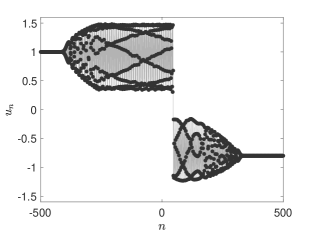
In section IV.4, we observed that a TDSW (a partial DSW connected to a traveling wave) is generated that transitions from the left level to the right level . By decreasing the value of below , a new wavetrain develops on the right level. Figure 19 shows three example profiles. When is close to the transition value , the excitation on top of the right level is small, see Figure 19(a). Decreasing further results in a larger amplitude wavetrain that resembles another TDSW; see Fig. 19(b). Close to , the wavetrains on the left and right levels approach binary oscillations, as shown in Fig. 19(c). Solution dynamics similar to those shown in Fig. 19(c), but with odd initial data, were studied extensively in [16]. In the work of [16], it is claimed that the emergence of blow up for the odd initial data they considered is “almost always” associated with the emergence of regions of binary oscillations for which the upper and lower oscillatory envelopes have opposite sign. Such a scenario was observed to result in the loss of hyperbolicity in the modulation equations (10) for binary oscillations and, consequently, a dynamical instability and thus exponential growth in a localized region of space that ultimately led to the finite time blow up of the wave pattern. For the Riemann data considered here (4), we numerically observe blow up in regions of the solution where binary oscillations are not apparent, which we now explore.
(a)
|
(b)
|
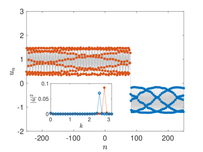
We will start with a more detailed discussion of the structure in Fig. 19(b) with , which is representative of many of the patterns found for and . A zoom-in of the solution in the co-moving frame near the shock interface is shown in Fig. 20 at three separate times () represented by different colors. Both the solution on the lattice (dots) and its zero-padded Fourier interpolant (curves) are shown with two different speeds. In Fig. 20(a) with speed , the leftmost wave at the three distinct times overlap, suggesting that it moves in the steady frame . Contrastingly, in Fig. 20(b) with speed , the rightmost wave at the three distinct times overlap, suggesting it moves in the slower steady frame . The spatial profile at and the Fourier transform of a 40-site window of the leftmost (rightmost) wave are shown in Fig. 21(a) in red (blue). Each wave has wavenumber concentration, and they are distinct ( for the left and for the right). This solution is a generalization of the unsteady shock (US) studied in section IV.5 in that two traveling waves are connected through a sudden jump. However, there are key differences. First, the shock interface itself is moving as shown in Fig. 20. Second, the frequency for the leftmost and rightmost waves are not identical, which can be seen in Fig. 21(c) that shows the time series at a node located at the left wave () and the right wave (). Here, it is clear that the oscillation frequencies are distinct. We conjecture that, much like the US, this wavetrain can be modeled by a discontinuous, weak solution of the Whitham equations satisfying the jump conditions (41). Rather than pursue this further, we instead turn to an examination of the large dynamics of the solution and, specifically, its eventual blow up.
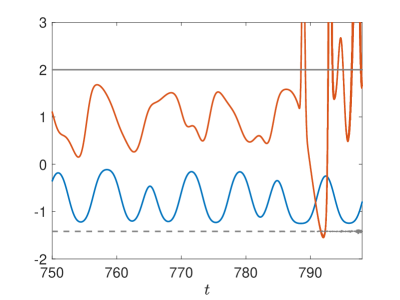
This structure is relatively coherent until about , after which small disturbances in the leftmost wave develop. Disturbances are noticeable if one compares the time series for (shown in Fig. 21(c)) and for (shown in Fig. 21(d)). At about the solution appears to experience finite-time blow up. Figure 22(a) shows the blow up. The spatial profile close to (but before) the time of blow up is shown in Fig. 21(b). Notice the location of the blow up is spatially concentrated within the leftmost wave and that the wavenumber of the traveling wave where the instability seems to manifest is about , (i.e., not a binary oscillation).
(a)
|
(b)
|
(c)
|
(d)
|
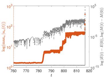
We conjecture that the observed blow up is due to an instability of the leftmost wave with wavenumber , and not due to numerical instability. A piece of evidence in this direction is that the mass and energy are conserved until times very close to the blow up time. The solid gray and dashed lines of Figs. 21(c,d) show the mass and energy , respectively. Note, in order for these quantities to be conserved, we employ periodic boundary conditions. For the simulations in this subsection, we concatenate the initial condition Eq. (4) with its reflection about the first site, leaving us with total nodes. Thus, the relevant window of space for the plots is only the second half of the lattice. We define the lattice indices so that the initial () jump from down to occurs at . This makes the plots consistent with those in the previous sections. We include the entire spatial window for the computation of and . Note that in Figs. 21(c,d) the quantities and are indeed conserved, even as the waveform begins to break down, see of panel Fig. 21(d). The gray solid and dashed lines of Fig. 22(a) show plots of and , respectively, for times leading to the blow up itself. While the energy remains constant after the strong onset of instability at about , the energy conservation breaks down for , while remains conserved. The conservation of mass in the numerical scheme is not surprising, since by direct computation one sees that the variational integrator applied to Eq. (35) with conserves the mass exactly [31]. The near conservation of energy for the variational integrator relies on the boundedness of the underlying numerical solution [54]. This will be clearly violated for solutions exhibiting collapse-type phenomena and thus it is not surprising that the energy is not conserved in the numerical scheme close to the time of blow up. Thus, it seems the initial collapse is due to instability of the wave (energy remains conserved for ), but after experiencing sustained large amplitude oscillations, the numerical scheme may begin to exhibit additional numerical instabilities (since energy is not conserved for ). The blow up time found here is an approximation that depends on the particulars of the numerical scheme.
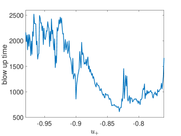
For and we observe a similar blow up of the solutions, with the blow up time varying roughly between and , see Fig. 22(b). We define the solution as blown-up once exceeds a large threshold. We practically used as the threshold (the actual threshold makes little difference in Fig. 22(b) since the blow up occurs so quickly). For this figure panel, we used a lattice size of and simulated until . We observe blow up with (at about ) but no blow up with , even when simulating until . This sharp transition between finite-time blow up and no blow up is further evidence that the blow up is due to an underlying instability of the waveform and not due to numerical instability.
The question of stability of traveling waves of this lattice is thus an important open question, meriting further investigation. Based on these findings, it appears that traveling waves with wavenumbers other than can lead to instabilities and finite-time blow up, a generalization of the findings in [16] where binary oscillations with were identified as a primary instability mechanism.
(a)
|
(b)
|
V Non-uniqueness of Riemann problems
As already mentioned in the introduction, the solutions to the Whitham system (31) are non-unique for certain classes of initial data. To discuss this in greater detail, we start with some preliminary comments concerning the inviscid Burgers’ PDE (1), which describes the dispersionless, hyperbolic scaling limit of the lattice (3) in the case of no oscillations and is a subsystem of (31) that governs the dynamics in the case of zero wave amplitude or zero wavenumber. To obtain an elementary example for non-uniqueness, we impose the odd initial condition
| (92) |
and notice that the rarefaction wave
| (96) |
is the unique self-similar solution according to the classical theory of hyperbolic conservation laws, see for instance [2]. The latter complements the PDE with an additional selection rules to exclude solutions that are considered to be unphysical. The most prominent example is the Lax condition for shocks but without such an admissibility criterion there exists a plethora of possibilities to fulfill the initial value problem (1)+(92). For instance, the formulas
| (107) |
provide two families of further self-similar solutions in dependence of the real parameter and , respectively, and contain (96) as limiting case for . The corresponding profile functions are illustrated in Figure 23 and combine a steady discontinuity at (which violates the Lax condition on both sides) with either two rarefaction waves or two Lax shocks.
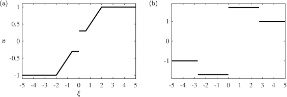
In numerical simulations of the lattice (3) we find a related family of solutions that differ only in microscopic details of the imposed initial conditions. As a typical but still elementary example we study the lattice initial data
| (111) |
where the free parameter reflects that the macroscopic Riemann data (92) can be realized in many different ways on the microscopic scale. Figure 24 reveals that the numerical solutions for different choices of correspond to distinct waves on the macroscopic scale. We always find a steady discontinuity at but its jump height as well as the other waves depend crucially on the value of microscopic parameter. In analogy to Figure 23 we observe two rarefaction waves in the case of but for we have to replace the Lax shocks by dispersive shock waves.
It remains a challenging task to understand the macroscopic impact of small-scale fluctuations in the initial data. For instance, it seems that the parameter in (111) determines the jump height of the emerging steady discontinuity in Figure 24 but we are not aware of any heuristic or even rigorous explanation thereof. Numerical simulations also indicate that microscopic details might not be relevant for Riemann data that are either positive or negative on both sides but also this must be investigated more thoroughly. Both issues are also intimately related to the properties of the Whitham system (33) which can be regarded as an extension of the Burgers’ equation (1). At least for sign changing Riemann problems, the lattice (3) is able to produce an entire family of Whitham solutions and it is very natural to investigate and classify them in terms of selection criteria and entropy inequalities. Moreover, other nonlinearities might produce further effects due to linearly degenerated states in the scalar first order PDE corresponding to (12); see [47, 55] for a related problem in FPUT chains whose force functions is increasing with inflection point.
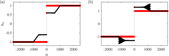
VI Conclusions and Future Challenges
In the present work, we revisit the first order nonlinear dynamical lattice of Eq. (12) through the lens of “lattice hydrodynamics” by providing a systematic analysis of the solutions to the canonical lattice Riemann problem (4) for the case of quadratic flux (3). Building on earlier works of [16, 31, 30], we have characterized dispersive shock waves and rarefaction waves, familiar from continuum dispersive hydrodynamics. But we also discover a variety of non-classical hydrodynamic-like solutions. In addition to finite time blow up, recognized earlier in the work of [16], we identify three additional dynamical regimes that are interpreted using a combination of numerical simulation, quasi-continuum approximation, and Whitham modulation theory. These regimes include the generation of a counterpropagating DSW and RW pair separated by a stationary, abrupt shock. Additionally, an abrupt, unsteady transition between two counterpropagating periodic waves with the same frequency is interpreted as a shock solution of the Whitham modulation equations. Finally, the phase diagram 1 of solutions to the lattice Riemann problem is rounded out by a traveling DSW (TDSW), consisting of an unsteady partial DSW, connected to a heteroclinic periodic-to-equilibrium traveling wave.
These elements of the lattice model’s phenomenology provide an opportunity to develop different aspects of the mathematical analysis of lattice hydrodynamics. For instance, we adapt the DSW fitting method of [49] to lattice equations in order to characterize the expansion and edge properties of lattice DSWs. We also follow up the work of [30], providing abstract modulation equations for a quasi-continuum analogue of the lattice dynamical system. We connect these to the genuinely discrete modulation equations, made explicit in the weakly nonlinear regime by a Poincaré-Lindstedt expansion of periodic traveling wave solution profiles and their frequencies. Hyperbolicity and self-similar solutions of the modulation equations are used to characterize lattice hydrodynamics. The quasi-continuum theory was also leveraged elsewhere, such as in characterizing the leading edge amplitude of the DSW and the periodic/traveling wave solutions of the discrete model. A truncation of the dynamics in wavenumber space allows for a linearized, large analysis of small amplitude oscillations that accompany the RW and DSW solutions.
Beyond the binary oscillations that have been studied previously, this work has identified new lattice hydrodynamic features that, so far, appear not to have a continuum, dispersive hydrodynamic parallel. Of particular interest is the rapid, unsteady transition between two in-phase counterpropagating periodic traveling waves with the same frequency (US in Fig. 1), identified with a shock solution of the Whitham modulation equations. This solution is born out of the bifurcation of another lattice solution particular to the lattice, the counterpropagating DSW, RW pair separated by a stationary shock (DSW+SS+RW in Fig. 1) when the DSW merges with the stationary shock. The US represents an unsteady generalization of the steady periodic-to-equilibrium heteroclinic solutions of higher order continuum dispersive equations, themselves interpreted as admissible shock solutions of the corresponding Whitham modulation equations [6, 50]. This work points to a new class of admissible “Whitham shocks” in the lattice context. It will be interesting to see if continuum solutions of this type also exist.
The asymptotic and semi-analytical tools used in this work constitute an effective framework in which to investigate the hydrodynamics of other lattice dynamical systems for which dispersive shock wave phenomena may arise. For example, the Riemann problem for FPUT chains generalizes to two wave families (second order in time) the problem of a single wave family studied here and has been shown to exhibit a variety of lattice hydrodynamic solutions including steady transition fronts [56] and DSWs [57].
A number of interesting open questions remain. Here, we list some of these. While the existence of periodic traveling waves has been proven [31], their stability and the existence, as well as stability of a more general class of traveling waves consisting of periodic-to-periodic heteroclinic solutions are important problems to better understand lattice hydrodynamics, with implications for finite time blow up and the construction of the TDSW solution. In the DSW+SS+RW solution, we have not been able to provide a mechanism that leads to the particular selection of the intermediate constant . We suspect that this is due to microscopic details of the lattice equation that have been neglected in the analysis. Of similar, unknown origin is the selection mechanism for shock solutions of the binary modulation equations (10) investigated in detail in [16]. On the other hand, the unsteady shock constitutes a genuine time-periodic orbit. Such periodic orbits are worthy of exploration in their own right, including from the perspective of dynamical systems by, for example, generalizing the spatial dynamics in dispersive [50] and dissipative [53] systems. The existence, stability and bifurcation analysis of such states are intriguing problems for future exploration. As discussed in [16], the model with quadratic flux (3) analyzed herein is one among several possible discretizations of the inviscid Burgers’ equation. A comparative study of different discretizations of the more general conservation law could lead to other lattice hydrodynamics and, in the case of integrable discretizations, be amenable to deeper mathematical analysis. These topics constitute some of the open problems within the theme of DSWs in one spatial dimension. The study of higher-dimensional models appears to be wide open. Some of these topics are currently under consideration and will be reported in future publications.
Acknowledgments
The authors would like to thank the Isaac Newton Institute for Mathematical Sciences for support and hospitality during the programme Dispersive Hydrodynamics when work on this paper was undertaken (EPSRC Grant Number EP/R014604/1). This material is also based upon work supported by the US National Science Foundation under Grants DMS-2107945 (C.C. and E.O.), DMS-2204702 (P.G.K.) and PHY-2110030 (P.G.K), DMS-2306319 (M.A.H.). This work began during P.S.’s time as INI-Simons Post Doctoral Research Fellow, and this author would like to thank the INI for support and hospitality during this fellowship, which was supported by Simons Foundation (Award ID 316017).
References
- [1] G.B. Whitham. Linear and Nonlinear Waves. Wiley, New York, 1974.
- [2] P. G. LeFloch. Hyperbolic systems of conservation laws. Lectures in Mathematics ETH Zürich. Birkhäuser Verlag, Basel, 2002. The theory of classical and nonclassical shock waves.
- [3] P. D. Lax and C. D. Levermore. The small dispersion limit of the Korteweg-de Vries equation: 1-3. Comm. Pure Appl. Math., 36(3,5,6):253–290; 571–593; 809–830, 1983.
- [4] A. V. Gurevich and L. P. Pitaevskii. Nonstationary structure of a collisionless shock wave. J. Exp. Theor. Phys., 65:590–604, 1973.
- [5] G.A. El and M.A. Hoefer. Dispersive shock waves and modulation theory. Physica D, 333:11, 2016.
- [6] P. Sprenger and M. A. Hoefer. Discontinuous shock solutions of the whitham modulation equations as zero dispersion limits of traveling waves. Nonlinearity, 33(7):3268, may 2020.
- [7] T. Congy, G. A. El, M. A. Hoefer, and M. Shearer. Dispersive Riemann problems for the Benjamin–Bona–Mahony equation. Stud. Appl. Math., 147(3):1089–1145, 2021.
- [8] T. Y. Hou and P. D. Lax. Dispersive approximations in fluid dynamics. Commun. Pure Appl. Math., 44(1):1–40, 1991.
- [9] M. Ehrnström, M. D. Groves, and E. Wahlén. On the existence and stability of solitary-wave solutions to a class of evolution equations of Whitham type. Nonlinearity, 25(10):2903–2936, 2012.
- [10] V. Y. Hur and M. A. Johnson. Modulational instability in the Whitham equation with surface tension and vorticity. Nonlinear Anal. Thoer., 129:104–118, 2015.
- [11] Adam L. Binswanger, Mark A. Hoefer, Boaz Ilan, and Patrick Sprenger. Whitham modulation theory for generalized Whitham equations and a general criterion for modulational instability. Stud. Appl. Math., 147(2):724–751, 2021.
- [12] T. B. Benjamin, J. L. Bona, and J. J. Mahony. Model Equations for Long Waves in Nonlinear Dispersive Systems. Phil. Trans. Roy. Soc. Lond. Ser. A, 272(1220):47–78, 1972.
- [13] P. Rosenau. Hamiltonian dynamics of dense chains and lattices: Or how to correct the continuum. Phys. Lett. A, 311:39, 2003.
- [14] P. Rosenau. Dynamics of nonlinear mass-spring chains near the continuum limit. Phys. Lett. A, 118:222, 1986.
- [15] V.F. Nesterenko. Dynamics of Heterogeneous Materials. Springer-Verlag, New York, 2001.
- [16] C. V. Turner and R. R. Rosales. The small dispersion limit for a nonlinear semidiscrete system of equations. Stud. Appl. Math., 99:205, 1997.
- [17] G.A. El, M.A. Hoefer, and M. Shearer. Dispersive and diffusive-dispersive shock waves for nonconvex conservation laws. SIAM Review, 59(1):3, 2017.
- [18] E. Hascoet and H. J. Herrmann. Shocks in non-loaded bead chains with impurities. Eur. Phys. J. B, 14:183, 2000.
- [19] E. B. Herbold and V. F. Nesterenko. Solitary and shock waves in discrete strongly nonlinear double power-law materials. Appl. Phys. Lett., 90(26):261902, 2007.
- [20] A. Molinari and C. Daraio. Stationary shocks in periodic highly nonlinear granular chains. Phys. Rev. E, 80:056602, 2009.
- [21] H. Kim, E. Kim, C. Chong, P. G. Kevrekidis, and J. Yang. Demonstration of dispersive rarefaction shocks in hollow elliptical cylinder chains. Phys. Rev. Lett., 120:194101, 2018.
- [22] S. Jia, W. Wan, and J. W. Fleischer. Dispersive shock waves in nonlinear arrays. Phys. Rev. Lett., 99:223901, Nov 2007.
- [23] Jian Li, S Chockalingam, and Tal Cohen. Observation of ultraslow shock waves in a tunable magnetic lattice. Phys. Rev. Lett., 127:014302, Jun 2021.
- [24] B. L. Holian. Atomistic computer simulations of shock waves. Shock Waves, 5(3):149–157, 1995.
- [25] D. H. Tsai and C. W. Beckett. Shock wave propagation in cubic lattices. J. of Geophys. Res., 71(10):2601, 1966.
- [26] George E. Duvall, R. Manvi, and Sherman C. Lowell. Steady Shock Profile in a One-Dimensional Lattice. Journal of Applied Physics, 40(9):3771–3775, 1969.
- [27] A. V. Gurevich and A. P. Meshcherkin. Expanding self-similar discontinuities and shock waves in dispersive hydrodynamics. Zhurnal Eksp. Noi Teor. Fiz., 87:1277–1292, 1984.
- [28] B. L. Holian and G. K. Straub. Molecular Dynamics of Shock Waves in Three-Dimensional Solids: Transition from Nonsteady to Steady Waves in Perfect Crystals and Implications for the Rankine-Hugoniot Conditions. Phys. Rev. Lett., 43(21):1598–1600, 1979.
- [29] M. E. Mossman, M. A. Hoefer, K. Julien, P. G. Kevrekidis, and P. Engels. Dissipative shock waves generated by a quantum-mechanical piston. Nat. Commun., 9(1):4665, 2018.
- [30] C. Chong, M. Herrmann, and P.G. Kevrekidis. Dispersive shock waves in lattices: A dimension reduction approach. Physica D, 442:133533, 2022.
- [31] M. Herrmann. Oscillatory waves in discrete scalar conservation laws. Math. Mod. Meth. Appl. S., 22(01):1150002, 2012.
- [32] E. Fermi, J. Pasta, and S. Ulam. Studies of Nonlinear Problems. I. Tech. Rep., (Los Alamos National Laboratory, Los Alamos, NM, USA):LA–1940, 1955.
- [33] G. B. Whitham. Exact solutions for a discrete system arising in traffic flow. P. Roy. Soc. A-Math-Phy., 428(1874):49–69, 1990.
- [34] Peter D. Lax. On dispersive difference schemes. Physica D, 18(1):250–254, 1986.
- [35] J. Goodman and P. D. Lax. On dispersive difference schemes. I. Commun. Pure Appl. Math., 41(5):591–613, 1988.
- [36] M Kac and Pierre van Moerbeke. On an explicitly soluble system of nonlinear differential equations related to certain toda lattices. Adv. Math., 16(2):160–169, 1975.
- [37] M. Toda. Theory of nonlinear lattices. Springer-Verlag, Berlin, 1989.
- [38] B.L. Holian, H. Flaschka, and D. W. McLaughlin. Shock waves in the Toda lattice: Analysis. Phys. Rev. A, 24:2595, 1981.
- [39] Y. Kodama. Solutions of the dispersionless Toda equation. Phys. Lett. A, 147(8):477–482, 1990.
- [40] A. Bloch and Y. Kodama. Dispersive regularization of the Whitham equation for the Toda lattice. SIAM J. on Appl. Math., 52(4):909–928, 1992.
- [41] S. Venakides, P. Deift, and R. Oba. The toda shock problem. Comm. Pure Appl. Math., 44(8-9):1171–1242, 1991.
- [42] G. Biondini, C. Chong, and P. Kevrekidis. On the Whitham modulation equations for the Toda lattice and the quantitative characterization of its dispersive shocks. arXiv:2312.10755, 2023.
- [43] S. Benzoni-Gavage, P. Noble, and L. M. Rodrigues. Slow Modulations of Periodic Waves in Hamiltonian PDEs, with Application to Capillary Fluids. J. Nonlinear Sci., 24(4):711–768, 2014.
- [44] A. M. Filip and S. Venakides. Existence and modulation of traveling waves in particles chains. Comm. Pure and Appl. Math., 52(6):693, 1999.
- [45] W. Dreyer, M. Herrmann, and A. Mielke. Micro-macro transition in the atomic chain via Whitham’s modulation equation. Nonlinearity, 19(2):471, 2005.
- [46] W. Dreyer and M. Herrmann. Numerical experiments on the modulation theory for the nonlinear atomic chain. Physica D, 237(2):255, 2008.
- [47] M. Herrmann and J. D. M. Rademacher. Riemann solvers and undercompressive shocks of convex FPU chains. Nonlinearity, 23:277, 2010.
- [48] C. M. Dafermos. Hyperbolic Conservation Laws in Continuum Physics. Springer, Berlin, 4th ed. edition, 2016.
- [49] G. A. El. Resolution of a shock in hyperbolic systems modified by weak dispersion. Chaos, 15(3):037103, 10 2005.
- [50] P. Sprenger, T. J. Bridges, and M. Shearer. Traveling Wave Solutions of the Kawahara Equation Joining Distinct Periodic Waves. J Nonlinear Sci, 33(5):79, 2023.
- [51] Alexander Mielke and C. Patz. Uniform asymptotic expansions for the fundamental solution of infinite harmonic chains. Z. Anal. Anwend., 36:437–475, 2017.
- [52] A M Kamchatnov. Nonlinear Periodic Waves and Their Modulations. World Scientific, 2000.
- [53] B. Sandstede and A. Scheel. Defects in oscillatory media: Toward a classification. SIAM J. Appl. Dyn. Syst., 3(1):1–68, 2004.
- [54] E. Hairer, S.P. Nørsett, and G. Wanner. Solving Ordinary Differential Equations I. Springer-Verlag, Berlin, Germany, 1993.
- [55] M. Herrmann and J. D. M. Rademacher. Heteroclinic travelling waves in convex FPU-type chains.
- [56] N. Gorbushin, A. Vainchtein, and L. Truskinovsky. Transition fronts and their universality classes. Phys. Rev. E, 106(2):024210, 2022.
- [57] C. Chong, A. Geisler, P. G. Kevrekidis, and G. Biondini. Integrable Approximations of Dispersive Shock Waves of the Granular Chain. arXiv:2402.08218, 2024.