On the global dynamics of a forest model with monotone positive feedback and memory
Franco Herrera
Sergei Trofimchuk
Instituto de Matemáticas, Universidad de Talca, Casilla 747, Talca, Chile
Abstract
We continue to study (see [6]) a renewal equation proposed in [1, 2] to model trees growth. This time we are
considering the case when the per capita reproduction rate is a non-monotone (unimodal) function of tree’s height . Note that
the height of some species of trees can impact negatively seed viability, cf. [3, p. 524], in a kind of autogamy depression.
Similarly to previous works, it is also assumed that the growth rate of an individual of height is a strictly decreasing function.
As in [5, 6], we analyse the connection between dynamics of the associated one-dimensional map , and the delayed (hence infinite-dimensional) model .
Our key observation is that this model is of monotone positive feedback type since is strictly increasing on independently on the monotonicity properties of .
keywords:
size-structured model, semiflow, global attractor, stability, Allee effect
††journal: MATRIX Annals
1 Introduction
In this note, we consider the renewal equation
(1)
where and functional is given by
This equation was proposed recently in [1, 2] to model trees growth and presents one of possible approaches to analyse the forest population dynamics, several other models are mentioned in [1, 2, 6]. In equation (1), function corresponds to the tree population birth rate at time ; continuous strictly decreasing function , , , is the growth rate of an individual of height ; represents the per capita death rate; globally Lipschitzian function , , is the per capita reproduction rate (depending only on height ). This model postulates the minimal height for all newborn trees. By [1, 2], gives the influx at originating from reproduction by the extant population. To ensure good persistence properties of solutions, it suffices to assume that a.e. on for some [6].
Clearly, (1) can be considered as an autonomous functional equation with infinite delay
once it is provided with non-negative initial conditions
, where belongs to the cone of non-negative measurable functions of the Banach space
with . It was proved in [1, 2, 6] that
the renewal equation (1) generates a continuous semiflow
by . It has a zero
steady state while the positive equilibria of are defined from the equation
(2)
Note that equation (2) has at least one positive solution if
and . If additionally increases on , then is strictly decreasing so that solution is unique, cf. [1, Theorem 4.1]. Moreover, this unique positive steady state is locally stable and globally attracting solution of (1), see
[1, 2, 6]. The key argument in proofs here is that semiflow is monotone [12] once is increasing on .
In some cases, however, the assumption of monotonicity of is not realistic. For example, the height of some species of trees can impact negatively seed viability, cf. [3, p. 524], in a kind of autogamy depression. Thus it would be interesting to study the dynamics in (1) in the case when
the per capita reproduction rate is a non-monotone (for instance, unimodal) function of tree’s height . Now, a general description of this dynamics is known from [6], where it was proven that under all assumed (except monotonicity of ) restrictions on , and
, , the semiflow has a compact global attractor
attracting each non-zero solution. Moreover, each element of satisfies
for some universal positive numbers .
In the sequel we present several analytical and numerical arguments shedding some light on possible dynamical structures of the global attractor without assumption of the monotonicity for . As in [5, 6], we will analyse the connection between dynamics of the associated one-dimensional map , and the delayed (hence infinite-dimensional) model .
2 Monotonicity of the function , .
Theorem 1
Assume all conditions (except monotonicity of ) imposed on and in Section 1. Then function
is strictly increasing on .
Proof 1
Assuming that a.e. on and setting and , we find that
Clearly, is strictly increasing and positive on , with ,
If , almost everywhere on , then
so that
Since is strictly decreasing, we find that the function
is continuous and strictly decreasing in for each fixed ,
Also, for a fixed and , it holds that
Thus the equation can be solved with respect to , we denote this solution by . Clearly, is strictly decreasing in the first argument and is strictly increasing in . Therefore is strictly decreasing in
In this way,
Particularly,
so that is a strictly increasing function independently on the monotonicity properties of .
\qed
Theorem 1 suggests to explore a possible connection between dynamical structures for the delayed equation (1) and seemingly simpler equation
(3)
where is a strictly increasing smooth function, for all , having three equilibria , . Equation (3) describes bounded solutions from the global attractor for the semiflow generated by the delayed equation
Specific applications of such a model can be found in neural network theory [7, 8]. Obviously, each equilibrium for (3) is determined from the equation
where the right hand side is given by a strictly increasing function. The global attractor
for (3) has relatively simple structure described in [8] (if is ”sufficiently unstable”, then is
a smooth solid 3-dimensional spindle separated by the invariant disk into the basins of attraction toward the tips and ). See also [9]
for further results and references on this topic.
3 Characteristic equations and principle of linearized stability
Formal linearization of the operator at an equilibrium yields the following action
Looking for the exponential eigenfunctions of the linearized equation , we obtain the characteristic equation for , cf. [1, 2]:
First, we consider the simpler case when is a non-decreasing function and (so that at the unique positive equilibrium):
Lemma 2
Assume that , , for and . Then the characteristic equation has exactly one real solution . Moreover, and for each other (complex) solution . If is strictly decreasing on , then .
Proof 2
The proof is obvious if a.e. so that we consider the case when . Clearly each eigenvalues satisfies the inequality . Taking into account opposite types of monotonicity of and and the fact that and , we deduce the existence of a unique real (non-positive) solution .
Assuming that there is another eigenvalue with , we get a contradiction:
Finally, suppose that is a strictly decreasing and .
Then we get the following contradiction:
Remark 3
Lemma 2 simplifies and improves arguments in [1, Section 5] (apparently, the uniqueness statement of this lemma contradicts to the existence of two negative eigenvalues in the particular case presented in [1, Subsection 5.1];
however, one of these eigenvalues is false and should be excluded to allow the convergence of integrals in .
Next, we analyse the situation when is not necessarily monotone function and (we assume that the model possesses at least one positive equilibrium ):
Lemma 4
Assume that is strictly decreasing Lipschitz continuous function on , . Then in the half-plane the characteristic equation has exactly one real solution and for each other (complex) solution . Moreover, if then , when and if .
Proof 3
Note that
Since
we obtain the following equivalent form of the characteristic equation:
The right side of this equation (we will denote it by , clearly
and ) is a strictly decreasing function of on the interval , , , so that the equation has exactly one real root on this interval.
Furthermore, we see that is a dominating eigenvalue. Indeed if is another eigenvalue with then
and we get a contradiction:
Finally, since we conclude that when , when and when . \qed
Lemma 4 implies that, except for the critical case , the local stability/instability of an equilibrium in (1) is equivalent to the local stability/instability of the same equilibrium for one-dimensional system :
Corollary 5
Assume that functions , have a bounded and globally Lipschitzian first derivative and . Then an equilibrium of continuous semiflow
is locally asymptotically stable if and is unstable when .
Proof 4
As it was established in [1, Theorem 3.1], under additional assumptions of this corollary, the functional is continuously differentiable with bounded derivative. Then an application of [1, Theorem 3.3] (based on Theorem 3.15 in [4]) completes the proof. \qed
Remark 6
Note that the inequalities and are equivalent, respectively, to the inequalities and , where
4 Numerical simulations and open problems
Stability analysis and discussion presented in the previous sections suggest
the existence of a ’large’ (we believe, open dense) set in the phase space
such that solutions with initial data from converge to one of stable equilibria. Thus we can expect that a typical numerical solution of equation (1) is asymptotically constant independently on the monotonicity properties of . To check this conclusion and to find out possible configurations for the set of equilibria for (1) with the unimodal fertility function , we took (which is used in the Nicholson blowflies equation and other models, cf. [10]); , , and , for some specific parameters . With these choices, our computations exhibit certain diversity in dynamical patterns for (1).
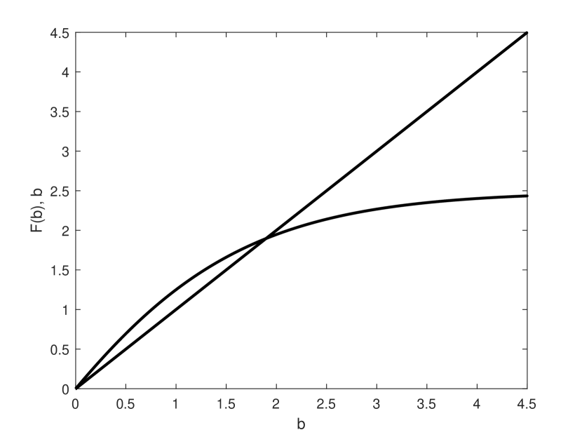
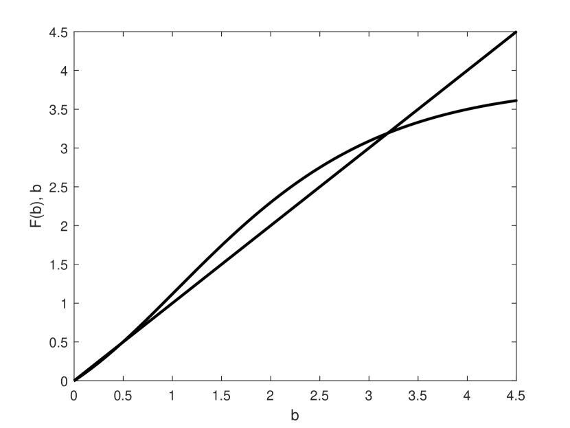
(a) and
(b) and
Figure 1: Graphics of and for different pairs of parameters and
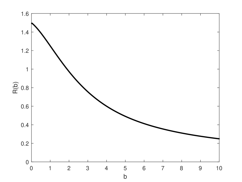
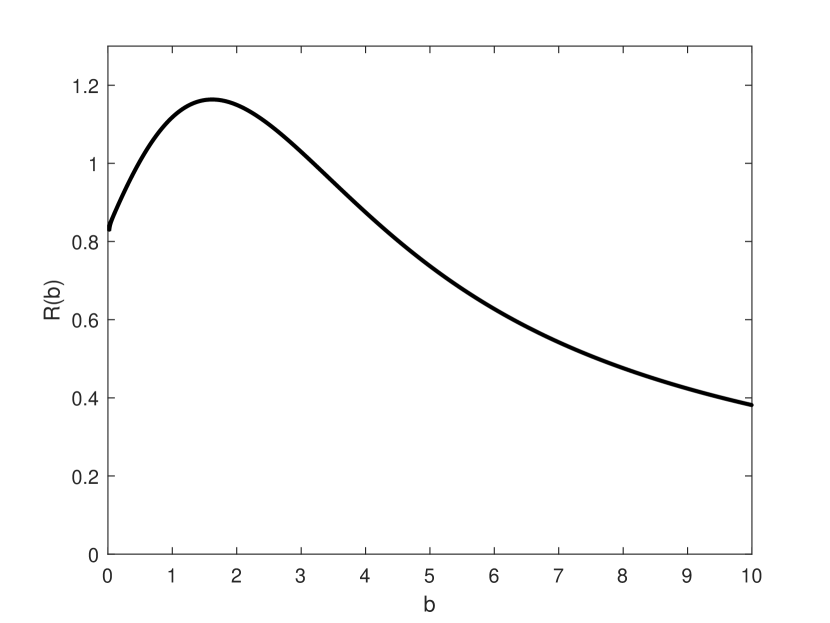
(a) and
(b) and
Figure 2: Graphics of for different pairs of parameters and
(c)
(d)
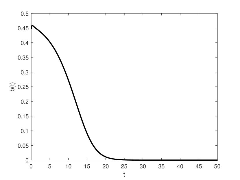
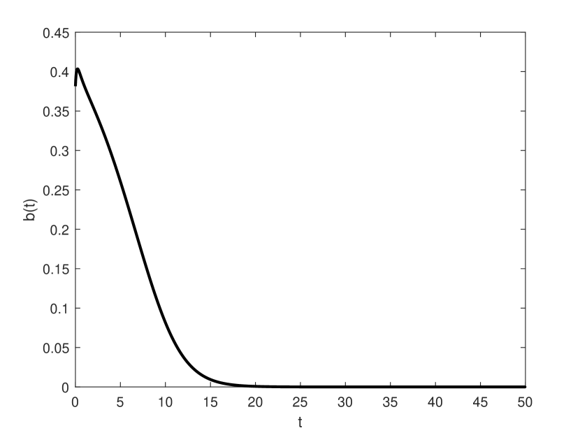
Figure 3: Simulations of using constant initial data
(a), and
(b), and
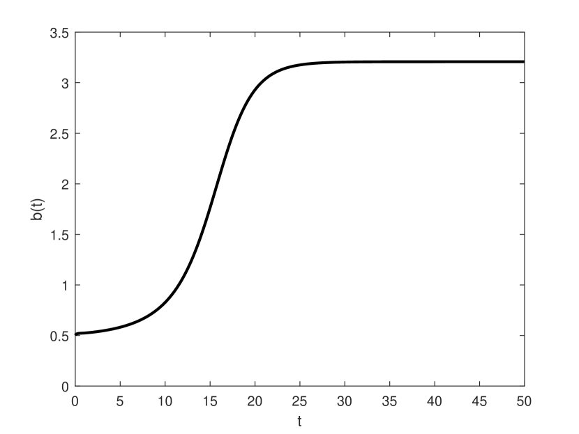
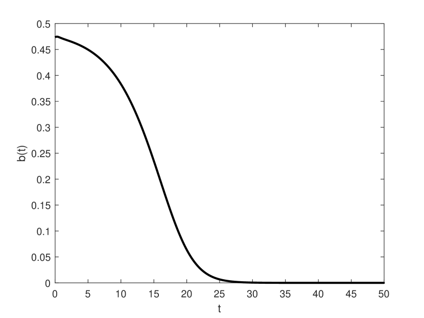
Figure 4: Simulations of using periodic initial data of the form
First, in full accordance with Theorem 1, Figure 1 shows that the function is strictly increasing even in lack of monotonicity for . Nevertheless, the function is not necessarily monotone and we can observe that for different values of , can be a decreasing function as well as a unimodal one, see Figure 4.
It is important to mention that these shapes for do not change essentially even if instead of we take with other orders of decay (e.g. polynomial) at .
Interestingly, regardless the fact , equation (1) with and has three equilibria, . Since , , , we deduce that equilibria and are locally asymptotically stable and is unstable (see Corollary 5). Our computations show that the linearization of (1) at has only one (real) eigenvalue with non-negative real part for , , therefore we cannot invoke the Hopf bifurcation approach to prove the existence of a periodic orbit for (1).
Simulating solutions of (1) for different initial data , we took constant and periodic initial functions close to the intermediate equilibrium . Figures 3 and 4 show that these solutions are asymptotically constant. Clearly, the nonlinearity is bistable here and we observe a kind of the Allee effect for the forest dynamics.
Acknowledgments
This research was supported in part by the projects FONDECYT 1231169 and AMSUD220002 (ANID, Chile). The first author was also supported by ANID-Subdirección de Capital Humano/Doctorado Nacional/2024–21240616.
The second author gratefully acknowledges the hospitality and the support of the MATRIX Institute allowing him to participate in the Research Program ”Delay Differential Equations and Their Applications” (Australia, Creswick, 12 –20 Dec 2023).
References
[1] C. Barril, À. Calsina, O. Diekmann, J. Z. Farkas, On competition through growth reduction, e-print arXiv:2303.02981,
https://doi.org/10.48550/arXiv.2303.02981
[2]
C. Barril, A. Calsina, O. Diekmann, J. Z. Farkas, On
hierarchical competition through reduction of individual growth, Journal of
Mathematical Biology, (2024) 88:66 https://doi.org/10.1007/s00285-024-02084-x
[3] M. A. Caraballo-Ortiz, E. Santiago-Valentín, T. A. Carlo,
Flower number and distance to neighbours affect the fecundity of Goetzea elegans (Solanaceae)
Journal of Tropical Ecology, 27 (2011) 521–528.
[4] O. Diekmann, M. Gyllenberg, Equations with infinite delay: blending the abstract and the concrete, J. Diff. Equations, 252 (2012), 819–851.
[5] F. Herrera, S. Trofimchuk, Dynamics of one-dimensional maps and Gurtin-MacCamy’s population model. Part I: asymptotically constant solutions, Ukrainian Math. J. 75 (2023), 1635–1651 https://doi.org/10.3842/umzh.v75i12.7678
[6] F. Herrera, S. Trofimchuk, Global dynamics of a size-structured forest model, e-print arXiv:2401.08618,
https://doi.org/10.48550/arXiv.2401.08618
[7] T. Krisztin, H.-O. Walther and J. Wu, Shape, smoothness and invariant stratification of an attracting set for delayed monotone positive feedback, Fields Institute Monograph Series, Vol. 11, AMS, Providence, RI, 1999.
[8] T. Krisztin, H.-O. Walther, Unique periodic orbits for delayed positive feedback and the global attractor.
J. Dyn. Differ. Equ. 13, 1–57 (2001).
[9] T. Krisztin, G. Vas, The unstable set of a periodic orbit for delayed positive feedback, J. Dyn. Differ. Equ. 28, (2016) 805–855.
[10] Z. Ma, P. Magal, Global asymptotic stability for Gurtin-MacCamy’s population dynamics model, Proceedings of the AMS,152 (2024), 765–780.
[11] J.A.J Metz, O. Diekmann, The dynamics of physiologically structured populations, Lecture Notes in Biomathematics, 68, 1986.