Estimating the Number of Components in Finite Mixture Models via Variational Approximation

Abstract

This work introduces a new method for selecting the number of components in finite mixture models (FMMs) using variational Bayes, inspired by the large-sample properties of the Evidence Lower Bound (ELBO) derived from mean-field (MF) variational approximation. Specifically, we establish matching upper and lower bounds for the ELBO without assuming conjugate priors, suggesting the consistency of model selection for FMMs based on maximizing the ELBO. As a by-product of our proof, we demonstrate that the MF approximation inherits the stable behavior (benefited from model singularity) of the posterior distribution, which tends to eliminate the extra components under model misspecification where the number of mixture components is over-specified. This stable behavior also leads to the $n^{-1/2}$ convergence rate for parameter estimation, up to a logarithmic factor, under this model overspecification. Empirical experiments are conducted to validate our theoretical findings and compare with other state-of-the-art methods for selecting the number of components in FMMs.

Keywords: Evidence lower bound; Mean-field approximation; Mixture models; Model selection; Singular models.

1 Introduction

One of the fundamental problems in statistics and machine learning is model selection, which attempts to select the most parsimonious model to fit the observed data from a list of candidate models. To address this problem, various model selection criteria have been proposed in the literature. Among them, two well-known criteria are the Akaike Information Criterion (AIC), proposed by Akaike, (1973), and the Bayesian Information Criterion (BIC), introduced by Schwarz, (1978). Under suitable conditions, AIC is known to lead to optimal prediction performance but tends to overestimate the model size; in comparison, BIC, which is derived as an asymptotic approximation to the log-marginal likelihood (a.k.a. model evidence) under a Bayesian framework, is able to consistently identify the true model (the model with the smallest size that contains the true data-generating process) as the sample size grows to infinity under the frequentist perspective, a property known as model selection consistency. The validity of BIC in approximating the model evidence requires the considered candidate model to be non-singular, meaning that its Fisher information matrix needs to be invertible at the true model parameter so that the maximum likelihood estimator (MLE) enjoys the asymptotic normality property. However, in many practical applications, especially when the considered model is over-specified, the Fisher information matrix is non-invertible, a situation referred to as singular models. Here, an over-specified model means that this model contains the true model, but the number of parameters in the model exceeds that of the true model; an accompanying notion is an under-specified model, where the model does not contain the true model.

In this paper, we consider the problem of model selection for a common and representative type of singular models, the finite mixture model (FMM), whose distribution family consists of all finite mixtures of probability distributions from a shared parametric family, with a fixed number of mixture components. FMMs have been extensively studied in the statistical literature (Titterington et al.,, 1985; McLachlan et al.,, 2019; Frühwirth-Schnatter,, 2006; Mengersen et al.,, 2011; Schlattmann,, 2009) and are widely applied in various fields, including agriculture, astronomy, biology, economics, engineering, and psychology, among others. In an FMM, the model size is determined by the number of components, which is typically unknown in practice. Thus, the model selection problem essentially becomes the task of identifying the minimal number of components required in the FMM to adequately fit the data. Over-specified FMMs are singular due to the non-identifiability of model parameters; in other words, different parameters can correspond to the same probability distribution. Over-specifying the number of components in an FMM also has the drawback of deteriorating the statistical efficiency of parameter estimation. For example, in a two-component Gaussian mixture model that is over-specified with the true model being a single Gaussian, the convergence rate of the MLE for estimating the location parameter decreases from the parametric rate $n^{-1/2}$ to $n^{-1/4}$, as shown by Chen, (1995); more generally, this rate of convergence further slows down with the inclusion of additional components (Ho and Nguyen, 2016a, ; Heinrich and Kahn,, 2018).

Extensions of BIC-type model selection criteria to singular models date back to a series of seminal works (Watanabe,, 2001; Yamazaki and Watanabe,, 2003; Yamazaki and Watanbe,, 2012) by Watanabe. In these works, tools from algebraic geometry, particularly those based on the resolution of singularities, are employed to determine the leading terms in the asymptotic expansion of the model evidence. The leading terms now depend on the real log canonical threshold (RLCT) and its multiplicity of the model; see Section 2.3 for a brief review or the recent book (Watanabe,, 2018) for further information. However, unlike the usual BIC that only depends on the considered model, the RLCT also requires knowledge of the true parameter value and therefore cannot be used in practice for model selection. Recently, Drton and Plummer, (2017) proposed a singular Bayesian information criterion (sBIC) for model selection in the context of singular models. This method involves solving a system of equations, the unique solution of which is shown to provide valid asymptotic approximations to the model evidences of candidate models. However, this approach requires knowledge of the real log canonical threshold (RLCT) and its multiplicity for all candidate models, the determination of which poses a highly challenging problem even in field of algebraic geometry. For example, for multi-variate Gaussian mixture models, their complete characterizations remain unresolved.

In this paper, we propose and analyze a new model selection approach for singular models based on variational Bayes (VB). VB has become a popular alternative to traditional sampling-based algorithms like MCMC for approximate Bayesian computation, owing to its computational scalability and good generalization performance in many applications. Our proposed approach draws inspiration from the recent work of Zhang and Yang, (2024), which shows that for non-singular models, the evidence lower bound (ELBO) derived from the mean-field (MF) approximation in variational Bayes can recover the leading terms in model evidence. Notably, the model selected by the ELBO tends to converge asymptotically with the one chosen by the BIC as the sample size increases. Furthermore, the calculation of the ELBO is a straightforward by-product of the Coordinate Ascent Variational Inference (CAVI) algorithm (see, e.g., Chapter 10 of Bishop,, 2006) for implementing the MF approximation. In particular, this approach eliminates the need for a case-by-case analysis to determine the effective number of parameters required in computing the BIC for non-singular models. In this work, we also consider the use of the ELBO from MF approximation for model selection in FMMs. Theoretically, we find that while the ELBO can no longer recover the leading term involving the RLCT in the model evidence, it still contains a term that penalizes over-specified models, leading to consistent model selection.

1.1 Related literature

In this subsection, we briefly review more recent works closely related to ours and defer a more extensive literature review and discussions to Appendix A. For Bayesian finite mixture models, Rousseau and Mengersen, (2011) studied the asymptotic behavior of posterior distributions in over-specified Bayesian FMMs, and proved that under certain conditions on the prior, the posterior tends to empty the extra components. Nguyen, (2013) and Guha et al., (2021) derived the contraction rate of posterior distributions on the parameters of interest in Bayesian FMMs under model misspecification; more reviews of literature on mixture model estimation can also be found therein. For variational Bayes (VB), recent works (Alquier and Ridgway,, 2020; Pati et al.,, 2018; Yang et al.,, 2020; Zhang and Gao,, 2020; Wang and Blei,, 2019; Zhang and Yang,, 2024) have provided general conditions under which VB leads to estimation consistency of the model parameter or data distribution, and derived the corresponding convergence rate. In particular, the theoretical framework developed in Yang et al., (2020) and Zhang and Yang, (2024) covers Bayesian latent variable models, including FMMs. Moreover, the theory in Pati et al., (2018) implies an $n^{-1/2}$ convergence rate, up to a logarithmic factor, for over-specified FMMs under the Hellinger metric, a result that will also play a key role in our proof. In the context of applying VB to Bayesian FMMs, Watanabe and Watanabe, (2006) derived upper and lower bounds for the ELBO (also called stochastic complexity therein) from the MF approximation for Bayesian Gaussian mixture models; also see Section 2.4 for further details. However, the gap between these two bounds does not ensure model selection consistency based on the ELBO. Watanabe and Watanabe, (2007) extended this analysis to general FMMs, but the issue of the gap remains unresolved. More recently, Bhattacharya et al., (2020) has shown that the ELBO from MF approximation recovers the leading term involving RLCT for a singular model in its normal-crossing form. However, while Hironaka’s theorem in algebraic geometry guarantees the existence of a reparametrization that can locally transform the posterior distribution of any singular model into its normal-crossing form, explicitly finding such a transformation is typically challenging.

1.2 Our contributions

In this study, we investigate the large sample properties of the ELBO derived from the MF variational approximation for FMMs under model misspecification. Specifically, we establish matching upper and lower bounds for the ELBO for a general class of FMMs whose constituting mixture components are exponential families. Our refined result will imply the consistency of model selection based on the ELBO. Moreover, unlike earlier analysis relying on conjugate priors to simplify the analysis, we only require the smoothness of the priors and employ Laplace approximation to analyze the conditional posterior distribution of parameters given latent class indicator variables. In our proof, we first establish a lower bound for the ELBO by constructing specific feasible solutions to the VB optimization problem, similar to those used by Watanabe and Watanabe, (2007). Our main technical contribution comes from our upper bound analysis. We utilize the variational risk bound under the Hellinger metric given by Pati et al., (2018) to identify certain important behaviors of the mixing weights, yielding a substantially improved upper bound that matches the lower bound up to high-order terms. Interestingly, our findings indicate that, unlike singular models in normal-crossing forms (Bhattacharya et al.,, 2020), directly applying MF to Bayesian FMMs does not recover the leading term in the model evidence, although it still results in consistent model selection. In addition, as a by-product of our analysis, we prove a corollary demonstrating that the MF variational approximation to the posterior distribution in Bayesian FMMs inherits the same interesting and stable behavior of tending to empty the extra components under model over-specification (Rousseau and Mengersen,, 2011). This stable behavior also leads to the $n^{-1/2}$ convergence rate for parameter estimation, up to a logarithmic factor, for those statistically identifiable components that do not empty out (see Section 3.3). It is also worth mentioning that our results do not require strong identifiability, as assumed by Rousseau and Mengersen, (2011) and Manole and Khalili, (2021), and are applicable to weakly identifiable FMMs (Ho and Nguyen, 2016a, ). Through experiments conducted on a location Gaussian mixture model and a real dataset, we empirically validate our theoretical findings and demonstrate that our model selection method is computationally efficient and tends to have higher power than existing state-of-the-art methods — it can correctly select the true number of components in FMMs using fewer samples.

The rest of the paper is organized as follows. Section 2 outlines the notation, provides background knowledge, formulates the problems we aim to address in this work and introduce our model selection method in finite mixture models. Section 3 lists our main assumptions and presents our main theoretical results about model selection via ELBO maximization and parameter estimation via mean-field variational approximation. Section 4 showcases simulated experiments of the Gaussian mixture model under various settings to complement our theoretical findings and reports results from a real data analysis. Finally, Section 5 concludes the paper with a discussion. Proofs and additional literature reviews are deferred to the appendices in the supplementary material.

2 Background and New Method

In this section, we begin with an overview of the notation, followed by a review of necessary background, and then introduce the problem formulation.

2.1 Notation

Throughout the paper, random variables are denoted by capital letters, while their realizations are represented by corresponding lowercase letters. For two probability measures $P$ and $Q$, let $p$ and $q$ be their Radon-Nikodym derivatives with respect to a $\sigma$-finite measure $\mu$, usually chosen as the Lebesgue measure or the counting measure. We denote the total variation and the (squared) Hellinger distance between $p$ and $q$ respectively as $d_{\rm TV}(p,q)=\frac{1}{2}\int|p-q|\,d\mu$ and $h^{2}(p,q)=\int(\sqrt{p}-\sqrt{q})^{2}\,d\mu$. Moreover, their Kullback-Leibler (KL) divergence is denoted as $D_{\rm KL}(p\|q)=\int p\log(p/q)\,d\mu$. We use $\mathcal{N}(\mu,\Sigma)$ to denote a (multivariate) normal distribution with mean $\mu\in\mathbb{R}^{d}$ and variance-covariance matrix $\Sigma\in\mathbb{R}^{d\times d}$. Additionally, for a vector $a\in\mathbb{R}^{d}$, we use $|a|$ to denote its Euclidean $\ell_{2}$-norm. Throughout this paper, we use $C$ to denote a generic positive constant whose value may vary from line to line. We also write $a\gtrsim b$ to mean $a\geq Cb$, $a\lesssim b$ to mean $a\leq Cb$ and $a\asymp b$ to mean $a\gtrsim b$ and $a\lesssim b$.

2.2 Singular models

In statistical learning, many classical techniques and conclusions are applicable primarily to regular models, such as the Laplace approximation, and the convergence rate and asymptotic normality of the maximum likelihood estimations (MLE). A statistical model $\mathcal{M}=\big{\{}p(\cdot\,|\,\theta)\,\big{|}\,\theta\in\Theta\big{\}}$ with parameter space $\Theta$ is called regular (or non-singular) if its parameter $\theta$ is identifiable and $p(\cdot\,|\,\theta)$ has a well-defined and positive definite Fisher information matrix $I(\theta)=\mathbb{E}_{\theta}[-\nabla^{2}\log p(X\,|\,\theta)]$ at each parameter $\theta\in\Theta$. In contrast, we say a model is singular when at least one of the conditions for regularity is not met. Many common statistical models are singular, such as finite mixture models, hidden Markov models, factor models, and neural networks. Mixture models, characterized by their ability to represent complex data distributions through convex combinations of simpler distributions from a shared parametric family, are a representative type of singular model. In this article, we focus exclusively on finite mixture models.

Concretely, let us start from a simple parametric family $\mathcal{G}=\big{\{}g(\cdot\,;\,\eta)\,\big{|}\,\eta\in\Omega\big{\}}$ parameterized by parameter $\eta\in\Omega$, whose parameter space $\Omega$ is a subset of $\mathbb{R}^{d}$, such as a location-scale family. For an integer $K$, a mixture model with $K$ components in $\mathcal{G}$ is model $\mathcal{M}_{K}=\big{\{}p(\cdot\,|\,\theta)\,\big{|}\,\theta=(w_{k},\eta_{k})_{k=1}^{K},\,\eta_{k}\in\Omega,\,w_{k}\geq 0,k\in[K]\mbox{ and }\sum_{k=1}^{K}w_{k}=1\big{\}}$ with

$$p(x\,|\,\theta)=\sum_{k=1}^{K}w_{k}\,g(x;\,\eta_{k}),\quad\theta=(w_{k},\eta_{k})_{k=1}^{K}\in\mathbb{R}^{dK+K},$$ (1)

where $\bm{w}=(w_{1},w_{2},\ldots,w_{K})\in[0,1]^{K}$ is called the mixing weight (vector) parameter, and, by slightly abusing the notation, we use $\bm{\eta}=(\eta_{1},\eta_{2},\ldots,\eta_{K})\in\Omega^{K}$ to denote the parameters associated with the $K$ mixture components. We also denote the corresponding (discrete) mixing distribution as $G(\theta)=\sum_{k=1}^{K}w_{k}\,\delta_{\eta_{k}}$, where $\delta_{\eta_{k}}$ denotes the Dirac mass at $\eta_{k}$. Generally, mixture models may lose identifiability, since different parameters may lead to the same data distribution $p(\cdot\,|\,\theta)$. However, $G(\theta)$ is always identifiable, that is, there is a one-to-one correspondence between $G(\theta)$ and $p(\cdot\,|\,\theta)$. This serves as one of the key assumptions in our theory (see Section 3.1). For example, the following two (Gaussian) mixture models correspond to the same standard normal distribution: $p(x\,|\,\theta_{1})=1\cdot\mathcal{N}(0,1)+0\cdot\mathcal{N}(1,1)$ and $p(x\,|\,\theta_{2})=\frac{1}{2}\cdot\mathcal{N}(0,1)+\frac{1}{2}\cdot\mathcal{N}(0,1)$. Fortunately, they still have the same mixing distribution $G(\theta_{1})=G(\theta_{2})=\delta_{0}$.

The loss of identifiability may lead to a non-invertible Fisher information matrix, resulting in decreased statistical efficiency — even when an identifiable submodel is considered, the best point estimator may suffer from a slow convergence rate as the sample size $n$ increases. For example, Chen, (1995) demonstrated such a phenomenon when the mixing distribution is restricted to the form $G(\theta)=\frac{2}{3}\delta_{-h}+\frac{1}{3}\delta_{2h}$ for $h\in\mathbb{R}$, and $g$ satisfies certain regular conditions to make the reduced parameter $h$ identifiable. However, even for this identifiable submodel, the MLE for $h$ still converges at the slow rate of $n^{-1/4}$ when the true parameter $h^{\ast}=0$. Therefore, it is crucial to correctly specify the number $K$ of mixture components before conducting statistical inference for finite mixture models, which motivates the problem of model selection for $K$ in this paper.

2.3 Model selection criteria for singular models

The Bayesian Information Criterion (BIC) is widely used for model selection for regular parametric models. Let $X^{n}=(X_{1},...,X_{n})$ be $n$ i.i.d. observations from the true model $p^{*}(x)$, which may or may not belong to the considered model $\mathcal{M}$. Under this setup, the BIC for a model $\mathcal{M}$ is derived as an asymptotic approximation to the so-called model evidence, or the log-marginal likelihood in a Bayesian framework, defined as

$$F(\mathcal{M})=\log\int_{\Theta_{\mathcal{M}}}\pi(\theta\,|\,\mathcal{M})\,p(X^{n}\,|\,\theta,\mathcal{M})\;d\theta=\underbrace{\log p(X^{n}\,|\,\widehat{\theta}_{\mathcal{M}},\mathcal{M})-\frac{d}{2}\log n}_{\mbox{\scriptsize BIC for model }\mathcal{M}}\,+\ \mathcal{O}_{P}(1),$$ (2)

where $\Theta_{\mathcal{M}}\in\mathbb{R}^{d}$ denotes its parameter space, $\pi(\theta\,|\,\mathcal{M})$ the prior density, $p(X^{n}\,|\,\theta,\mathcal{M})$ the likelihood function, and $\widehat{\theta}_{\mathcal{M}}=\operatorname*{arg\,max}_{\theta\in\Theta_{\mathcal{M}}}p(X^{n}\,|\,\theta,\mathcal{M})$ is the MLE of $\theta$ under model $\mathcal{M}$. The BIC in the preceding display consists of two terms: a model goodness-of-fit term and an additional term of $-\frac{d}{2}\log n$ resulting from the integration over $\mathbb{R}^{d}$, which penalizes larger models that may lead to overfitting. It is a classical result (Schwarz,, 1978) that selecting a model based on maximizing BIC enjoys the model selection consistency property. Unfortunately, for singular models with non-invertible Fisher information matrices, the asymptotic expansion (2) for the model evidence no longer holds, as the effective dimension of the parameter space is no longer equal to the number $d$ of parameters.

In a seminal work, Watanabe, (2001) employed algebraic geometry tools to show that for a singular model $\mathcal{M}$, the asymptotic behavior of the log-marginal likelihood can be characterized through

$$F(\mathcal{M})=\log p^{*}(X^{n})-\lambda_{\mathcal{M}}\log n+(m_{\mathcal{M}}-1)\log\log n+\mathcal{O}_{P}(1),$$ (3)

where $\lambda_{M}$ is called the real log canonical threshold (RLCT) of model $\mathcal{M}$ that determines the effective number of parameters, and $m_{\mathcal{M}}$ is its multiplicity. Leveraging this general result, Drton and Plummer, (2017) proposed a model selection method by maximizing a singular Bayesian information criterion (sBIC), which is computed by solving a system of equations whose unique solution approximates the leading terms in $F(\mathcal{M})$. However, this approach requires knowledge of the real log canonical threshold (RLCT) and its multiplicity for all candidate models, the determination of which is a highly nontrivial problem even in the field of algebraic geometry within pure mathematics.

2.4 Selecting number of components in mixture models via variational approximation

To handle the analytically intractable integral in $F(\mathcal{M})$, variational inference attempts to approximate $F(\mathcal{M})$ defined in (2) from below by utilizing Jensen’s inequality (to $-\log(t)$),

$$\log\int_{\Theta_{\mathcal{M}}}\frac{\pi(\theta\,|\,\mathcal{M})\,p(X^{n}\,|\,\theta,\mathcal{M})}{q_{\theta}(\theta)}\,q_{\theta}(\theta)\,d\theta\geq\int_{\Theta_{\mathcal{M}}}q_{\theta}(\theta)\log\frac{\pi(\theta\,|\,\mathcal{M})\,p(X^{n}\,|\,\theta,\mathcal{M})}{q_{\theta}(\theta)}\,d\theta:\,=\mathcal{L}(q_{\theta}),$$

where $q_{\theta}(\theta)$ is a distribution from a tractable distribution family $\Gamma$ for approximating the posterior distribution $p(\theta\,|\,X^{n},\mathcal{M})$. We will focus on the commonly used mean-field family $\Gamma_{\rm MF}$ in this work, where $q_{\theta}$ factorizes over the (blocks of) components of $\theta$. The evidence lower bound (ELBO) is then defined as the best approximation to $F(\mathcal{M})$ by maximizing the lower bound $L(q_{\theta})$ over $q_{\theta}\in\Gamma_{\rm MF}$. In the rest of the paper, when we consider a fixed model $\mathcal{M}$, we may suppress $\mathcal{M}$ in our notation for simplicity.

Now let us specialize the above general framework to finite mixture models (1). As a common practice, we will augment the mixture model into a hierarchical model via introducing latent (class indicator) variables to facilitate efficient computation. In fact, a key property utilized in our theoretical analysis is that the conditional distribution of observation given latent variable is a regular parametric model. Let $S^{n}=(S_{1},...,S_{n})$ denoting the collection of all latent variables, with each $S_{i}$ being discrete and taking values from $\{1,..,K\}$, indicating which mixture component that $X_{i}$ comes from. Then we have the hierarchical form of the model as $[X_{i}\,|\,S_{i}=k]\overset{iid}{\sim}g(x\,;\,\eta_{k})$ and $S_{i}$ are i.i.d. with $P(S_{i}=k)=w_{k}$, for $i\in[n]$ and $k\in[K]$. Moreover, we can express the joint distribution of $X^{n}$ given $\theta$ as

$$p(X^{n}\,|\,\theta)=\sum_{s^{n}\in[K]^{n}}p(X^{n}\,|\,s^{n},\theta)\,p(s^{n}\,|\,\theta)=\prod_{i=1}^{n}\sum_{s_{i}\in[K]}p(X_{i}\,|\,s_{i},\eta)\,p(s_{i}\,|\,w).$$

Let $Z^{n}=(\theta,S^{n})$ denote the collection of all hidden variables, then the augmented posterior distribution $p(Z^{n}\,|\,X^{n})$ satisfies $p(\theta,s^{n}\,|\,X^{n})\varpropto p(X^{n},s^{n}\,|\,\theta)\,\pi(\theta)$. Now the variational inference will use $q_{Z^{n}}\in\Gamma$ to approximate the joint posterior distribution $p(Z^{n}\,|\,X^{n})$ (by replacing $\theta$ with $Z^{n}$ therein). To reduce the approximation error, we consider the block MF approximation where $\Gamma_{\rm MF}=\big{\{}q_{Z^{n}}=q_{\theta}\otimes q_{S^{n}}\big{\}}$. Let $\widehat{q}_{Z^{n}}=\widehat{q}_{\theta}\otimes\widehat{q}_{S^{n}}:=\operatorname*{arg\,max}_{q_{Z^{n}}\in\Gamma_{\rm MF}}\mathcal{L}(q_{Z^{n}})$ denote the best variational density that approximates $p(Z^{n}\,|\,X^{n})$, and the corresponding $\mathcal{L}(\widehat{q}_{Z^{n}})$ is the ELBO for the mixture model with $K$ components. Then the best variational approximation to its posterior $p(Z^{n}\,|\,X^{n})$ is defined as the minimizer of the following KL divergence,

$$\widehat{q}_{Z^{n}}:=\mathop{\arg\inf}\limits_{q_{Z^{n}}\in\Gamma}D_{\rm KL}\big{(}q_{Z^{n}}(\cdot)\,\big{\|}\,p(\cdot\,|X^{n})\big{)}.$$ (4)

Note that for any $q_{Z^{n}}$, we have the following relationship

$$D_{\rm KL}\big{(}q_{Z^{n}}(\cdot)\,\big{\|}\,p(\cdot\,|X^{n})\big{)}=\log\int p(X^{n}|\theta)\,\pi(\theta)\,d\theta-\mathcal{L}(q_{Z^{n}})\geq 0,$$

where the first term is the evidence and the second term

$$\mathcal{L}(q_{Z^{n}})=\int q_{Z^{n}}(z^{n})\log\frac{p(X^{n},s^{n}|\theta)\,\pi(\theta)}{q_{Z^{n}}(z^{n})}dz^{n}.$$ (5)

is the corresponding ELBO function, since the KL divergence is non-negative. Therefore, maximizing the ELBO over $q_{Z^{n}}$ is equivalent to minimizing the KL divergence. In addition, the ELBO valued at its maximizer $\widehat{q}_{Z^{n}}(z^{n})$ is a potential surrogate to the model evidence in singular model selection, as long as this approximation retains some characteristics of the evidence. As aforementioned, a commonly used variational family $\Gamma$ is the (block) mean-field (MF) approximation, where $q_{Z^{n}}(z^{n})$ is factorized as

$$q_{Z^{n}}(z^{n})=q_{\theta}(\theta)\otimes q_{S^{n}}(s^{n}).$$ (6)

We will focus on the MF, and use $\widehat{q}_{Z^{n}}$ to denote the maximizer of the ELBO function $\mathcal{L}(\cdot)$, which, according to the MF definition, can be further decomposed into $\widehat{q}_{Z^{n}}=\widehat{q}_{\theta}\otimes\widehat{q}_{S^{n}}$. We will refer to $\widehat{q}_{Z^{n}}$ as the variational posterior (distribution). If we use $\widehat{\mathcal{L}}_{K}=\mathcal{L}_{K}(\widehat{q}_{Z^{n}})$ to denote the (maximal) ELBO value under the FMM with $K$ components, then our selected number of components $\widehat{K}$ via ELBO maximization can be defined via

$$\widehat{K}=\operatorname*{arg\,max}_{K}\widehat{\mathcal{L}}_{K}.$$ (7)

Regarding the block MF approximation, the following theorem gives a necessary condition for $\widehat{q}_{Z^{n}}$ to be the maximizer of the ELBO, as stated in the Theorem 2.1 by Beal, (2003). This theorem provides a system of distributional equations determining $\widehat{q}_{\theta}(\theta)$ and $\widehat{q}_{S^{n}}(s^{n})$, which plays an important role and will be repeatedly used in our proofs.

Theorem 1

Under the block MF approximation, the variational posterior $\widehat{q}_{Z^{n}}=\widehat{q}_{\theta}\otimes\widehat{q}_{S^{n}}$ satisfies

$$\widehat{q}_{\theta}(\theta)=\frac{1}{\widehat{C}_{r}}\pi(\theta)\exp\bigg{\{}\sum_{s^{n}\in[K]^{n}}{\widehat{q}_{S^{n}}(s^{n})}\log p(X^{n},s^{n}\,|\,\theta)\bigg{\}}$$ (8)

$$\mbox{and}\quad\widehat{q}_{S^{n}}(s^{n})=\frac{1}{\widehat{C}_{Q}}\exp\bigg{\{}\int{\widehat{q}_{\theta}(\theta)}\log p(X^{n},s^{n}\,|\,\theta)\,d\theta\bigg{\}},$$ (9)

where $\widehat{C}_{r}$ and $\widehat{C}_{Q}$ are the normalization constants.

Under the above settings, Watanabe and Watanabe, (2007) derived upper and lower bounds for $\mathcal{L}(\widehat{q}_{Z^{n}})$ under a symmetric Dirichlet prior Diri$(\phi_{0},\ldots,\phi_{0})$, $\phi_{0}\geq 0$, on the mixing weights $w$ and a conjugate prior for the parameters $\eta$ associated with mixture components from an exponential family. Specifically, if we denote the variational posterior mean (estimator) of $\theta$ as $\overline{\theta}:=\int\theta\,\widehat{q}_{\theta}(\theta)\,d\theta$, then Watanabe and Watanabe, (2007) proved that (after some notation adaptions)

$$\log p^{*}(X^{n})-\underline{\lambda}\log n+\mathcal{O}_{P}(1)\leq\mathcal{L}(\widehat{q}_{Z^{n}})\leq\log p^{*}(X^{n})-\overline{\lambda}\log n+\log\frac{p(X^{n}\,|\,\overline{\theta})}{p^{*}(X^{n})}+\mathcal{O}_{P}(1)$$

as sample size $n$ tends to infinity, and the leading coefficients $\underline{\lambda}$ and $\overline{\lambda}$ are given by

$$\underline{\lambda}=\begin{cases}(K-K^{*})\phi_{0}+\frac{dK^{*}+K^{*}-1}{2},&\phi_{0}\leq\frac{d+1}{2},\\ \frac{dK+K-1}{2},&\phi_{0}>\frac{d+1}{2};\end{cases}\quad\mbox{and}\quad\overline{\lambda}=\begin{cases}(K-1)\phi_{0}+\frac{d}{2},&\phi_{0}\leq\frac{d+1}{2},\\ \frac{dK+K-1}{2},&\phi_{0}>\frac{d+1}{2},\end{cases}$$

where $K^{*}$ denotes the true number of components underlying the data-generating process. When $\phi_{0}<(d+1)/2$, there exists a gap between $\underline{\lambda}$ and $\overline{\lambda}$. It should be noted that $(d+1)/2$ also serves as the threshold for $\phi_{0}$, below which the desirable stable behavior of the posterior distribution and its variational approximation (see Corollary 5) to empty the extra components can be maintained. This stable behavior is also shown to lead to improved parameter estimation efficiency (see Theorem 7). In contrast, when $\phi_{0}>(d+1)/2$ and $K$ is over-specified, then two or more components can be very close with non-negligible weights each, leading to unstable and less accurate parameter estimation (for example, see our numerical results in Section 4.1). In practice, a choice of $\phi_{0}$ less than one is also typically preferred in the literature. For example, a default choice of $\phi_{0}$ in topic models (Blei et al.,, 2003) is $K^{-1}$, which encourages a sparse mixing weight $w$ for easier interpretation. Conversely, a larger $\phi_{0}$ tends to promote a denser mixing weight; in particular, Diri$(\phi_{0},\ldots,\phi_{0})$ tends to concentrate around the uniform weights $(K^{-1},\ldots,K^{-1})$ as $\phi_{0}$ approaches infinity. Therefore, it is an important theoretical question whether this gap can be eliminated for small $\phi_{0}$, so that model selection based on maximizing the ELBO is provably consistent. In this work, we close this gap by proving matching lower and upper bounds for the ELBO under any positive values of $\phi_{0}$. The discussion following our Theorem 2, Section 3.3, and our numerical results (e.g., Section 4.1) both suggest that a small $\phi_{0}$ value is indeed preferred for accurate model selection and parameter estimation.

3 Theoretical Results

In this section, we present our main theoretical results. Here, we assume that the dataset $X^{n}=(X_{1},...,X_{n})$ consists of $n$ observations that are i.i.d. samples from a fixed true data-generating process $p^{*}(x)=\sum_{k=1}^{K^{*}}w_{k}^{*}g(x;\eta_{k}^{*})$, where $K^{*}$ denotes the true component number, and $\theta^{*}=(w_{k}^{*},\,\eta_{k}^{*})_{k=1}^{K^{*}}\in\mathbb{R}^{dK^{*}+K^{*}}$ denotes the (unique) true parameters under the mixture model (1) with $K^{*}$ components, where all $\eta_{k}$’s are distinct and $\min_{k\in[K^{*}]}w_{k}^{\ast}>0$. Let $G^{*}$ denote the corresponding mixing measure for the truth. Throughout this section, we consider a finite mixture model with $K\geq K^{*}$ components. In addition, we follow the literature by assuming the parametric family $\mathcal{G}=\big{\{}g(\cdot\,;\,\eta)\,\big{|}\,\eta\in\Omega\big{\}}$ for the mixture components to be an exponential family in the canonical form, that is, $g(x;\eta)=\exp\big{\{}\eta^{T}T(x)-T_{0}(x)-A(\eta)\big{\}}$, where $\eta\in\mathbb{R}^{d}$ is the natural parameter, $T(x)$ is the sufficient statistic and $A(\eta)$ is the log-partition function. The Fisher information matrix for this exponential family is $I(\eta)=\nabla^{2}A(\eta)$, which implies the convexity of $A(\eta)$ over its domain $\mathbb{R}^{d}$. Consequently, the log-likelihood function $\log g(x;\eta)$ is concave with respect to $\eta$ for all $x$. One important assumption of our theory (see Section 3.1 below) is the relationship between total variation and Wasserstein-type distances in FMMs, which transforms the closeness of mixture models in density functions into closeness in their mixing measure or model parameters. Such a relationship can be verified for most commonly used FMMs; see Section 3.4 for concrete examples. An $r$-th order Wasserstein distance (or simply $r$-Wasserstein distance) between two mixing measures $G(\theta)=\sum_{k=1}^{K}w_{k}\,\delta_{\eta_{k}}$ and $G(\theta^{\prime})=\sum_{k=1}^{K^{\prime}}w^{\prime}_{k}\,\delta_{\eta^{\prime}_{k}}$ is defined as:

$$W_{r}\big{(}G(\theta),G(\theta^{\prime})\big{)}=\Big{(}\inf_{q_{ij}}\sum_{i,j}q_{ij}|\eta_{i}-\eta_{j}^{\prime}|^{r}\Big{)}^{1/r},$$ (10)

where the infimum is taken over all nonnegative probability masses $\big{\{}q_{ij}:\,i\in[K],\,j\in[K^{\prime}]\big{\}}$ satisfying two marginal constraints $\sum_{i=1}^{K}q_{ij}=w^{\prime}_{j}$ for $j\in[K^{\prime}]$ and $\sum_{j=1}^{K^{\prime}}q_{ij}=w_{i}$ for $i\in[K]$.

3.1 Assumptions

Recall that we have the symmetric Dirichlet distribution Diri$(\phi_{0},\ldots,\phi_{0})$, $\phi_{0}>0$ as our prior for the mixing weights $w$, whose density takes the form of $\pi(\bm{w})=\frac{\Gamma(K\phi_{0})}{\Gamma(\phi_{0})^{K}}\prod^{K}_{k=1}w_{k}^{\phi_{0}-1}$, for all $\bm{w}=(w_{1},\ldots,w_{K})\in[0,1]^{K}$ such that $\sum_{k=1}^{K}w_{k}=1$, where $\Gamma(\cdot)$ is the Gamma function. We also consider independent priors on $\eta$, that is, $\pi(\bm{\eta})=\prod_{k=1}^{K}\pi(\eta_{k})$, $\eta_{k}\in\Omega$, where for each $k$, the density $\pi(\eta_{k})$ is twice continuously differentiable on $\Omega$. In addition, we make the following assumptions.

Assumption A: Recall that $p^{*}$ is the true data-generating probability with mixing measure $G^{*}$ and has $K^{*}$ components.

1. (Parameter space compactness) The parameter space $\Omega$ of mixture components is a compact subset of $\mathbb{R}^{d}$, i.e., there exists a constant $L<\infty$ such that $\sup_{\eta,\eta^{\prime}\in\Omega}|\eta-\eta^{\prime}|\leq L$.

2. (Regularity of mixture component family) There exist two positive constants $a$ and $b$ such that $y^{T}I(\eta)\,y\in[a,b]$ over all $|y|=1$ and all $\eta\in\Omega$, where $I(\eta)=\nabla^{2}A(\eta)$ is the Fisher information matrix for the mixture components.

3. (Identifiability of mixing measure) The total variation distance between any FMM $p(x|\theta)$ with $K(\geq K^{\ast})$ components and the true model $p^{\ast}$ satisfies $d_{\rm TV}\big{(}p(\cdot\,|\theta),p^{*}(\cdot)\big{)}=0$ if and only if its mixing measure $G(\theta)$ satisfies $G(\theta)=G^{*}$. Moreover, there exist an positive integer $r$ and positive constants $\varepsilon$ and $c_{0}$ such that $d_{\rm TV}\big{(}p(\cdot\,|\theta),p^{*}(\cdot)\big{)}\geq c_{0}W_{r}^{r}\big{(}G(\theta),G^{*}\big{)}$ for any $p(\cdot\,|\theta)$ with mixing measure $G(\theta)$ (with $K$ components) satisfying $W_{r}\big{(}G(\theta),G^{*}\big{)}<\varepsilon$.

Assumption A1 is commonly made in the literature for technical simplicity when analyzing singular models. Assumption A2 is a mild condition with $\Omega$ being compact and is satisfied by all non-singular (i.e., not curved) exponential families. Assumption A3 requires certain partial identifiability for the true model $p^{*}$ with $K^{*}$ components. It essentially states that for any mixing measure $G(\theta)$ sufficiently close to $G^{*}$, the total variation of the density functions is lower bounded by some Wasserstein-type distance between the mixing measures. For example, if the family ${g(x;\eta),\eta\in\Omega}$ is identifiable in the second-order (see Definition 3.2 in (Ho and Nguyen, 2016b, )), in other words, $g(x;\eta_{k})$ and their derivatives with respect to $\eta_{k}$ up to the second order are linearly independent, then Assumption A3 is satisfied with $r=2$. For families that are not identifiable in the second-order, for instance, the location-scale Gaussian distributions, verification of Assumption A3 can be done in a case-by-case manner, where $r$ may also depend on $K^{*}$ and $K$. See Section 3.4 for more examples that satisfy these assumptions.

It is also worth noting that, with Assumptions A1 and A3, the (localized) inequality in the second part of Assumption A3 can be made global. Specifically, there exists a constant $c_{1}$ such that $d_{\rm TV}(p(\cdot\,|\theta),p^{*}(\cdot))\geq c_{1}W_{r}^{r}(G(\theta),G^{*})$ for all possible $\theta$. The proof is straightforward. Let $\mathcal{A}:=\{\theta:W_{r}(G(\theta),G^{*})\geq\varepsilon,\bm{\eta}\in\Omega^{K}\}$. Since $W_{r}(G(\theta),G^{*})$ is continuous in $\theta$, $\mathcal{A}$ is a compact set and $d_{\rm TV}(p(\cdot\,|\theta),p^{*}(\cdot))>0$ on $\mathcal{A}$ by the first part of Assumption A3. For the considered exponential family, the total variation is also a continuous function with respect to $\theta$. Therefore, it attains a strictly positive infimum on $\mathcal{A}$, which we denote as $\tau:=\inf_{\theta\in\mathcal{A}}d_{\rm TV}(p(\cdot\,|\theta),p^{*}(\cdot))>0$. Meanwhile, from Assumption A1, we have $W_{r}^{r}(G(\theta),G^{*})\leq L^{r}$. Therefore, on $\mathcal{A}$, we also have $d_{\rm TV}(p(\cdot\,|\theta),p^{*}(\cdot))\geq(\tau/L^{r})W_{r}^{r}(G(\theta),G^{*})$. Letting $c_{1}=\min\{c_{0},\tau/L^{r}\}$, it then follows from above and the second part of Assumption A3 that for any $\theta$, we have:

$$d_{\rm TV}\big{(}p(\cdot\,|\theta),p^{*}(\cdot)\big{)}\geq c_{1}W_{r}^{r}\big{(}G(\theta),G^{*}\big{)},$$ (11)

which provides a global inequality relating the two distance metrics over any compact set. The above argument allows us to avoid assuming a reverse inequality $d_{\rm TV}(p(\cdot\,|\theta),p^{*}(\cdot))\leq c_{0}W_{r}^{\alpha}(G(\theta),G^{*})$ for some $\alpha>0$ and for any $p(\cdot\,|\theta)$ with mixing measure $G(\theta)$ in order to extend the local inequality into a global one, as was done in Corollary 3.1 of Ho and Nguyen, 2016b .

3.2 Large sample properties of ELBO

Now we are ready to present our first main result as follows, which provides two-sided bounds to the ELBO $\mathcal{L}(\widehat{q}_{Z^{n}})$ with matching leading terms. Recall that we use $\overline{\theta}:=\int\theta\,\widehat{q}_{\theta}(\theta)\,d\theta$ to denote the variational point estimator for $\theta$.

Theorem 2 (Finite-sample two-sided bound of ELBO)

Suppose Assumptions A1–A3 hold and $K\geq K^{*}$. Then there exist some positive constants $C_{1}$, $C_{2}$ and $c$ independent of $n$ such that with probability at least $1-n^{-c}$, we have

$$\log p^{*}(X^{n})-\lambda\log n+C_{1}\leq\mathcal{L}(\widehat{q}_{Z^{n}})\leq\log p^{*}(X^{n})-\lambda\log n+\log\frac{p(X^{n}\,|\,\overline{\theta})}{p^{*}(X^{n})}+C_{2},$$

where $C_{1}=K\log\Gamma(\phi_{0})-\Gamma(K\phi_{0})-C$ and $C_{2}=K\log\Gamma(\phi_{0})-\Gamma(K\phi_{0})+C$ for some constant $C$ independent of $(n,\phi_{0})$, and $\lambda$ is given by

$$\lambda=\begin{cases}(K-K^{*})\phi_{0}+\frac{dK^{*}+K^{*}-1}{2},&\phi_{0}\leq\frac{d+1}{2},\\ \frac{dK+K-1}{2},&\phi_{0}>\frac{d+1}{2}.\end{cases}$$ (12)

We note that $K\log\Gamma(\phi_{0})-\Gamma(K\phi_{0})$ is an increasing function with respect to both $K$ and $\phi_{0}$. In particular, a large $\phi_{0}$ may cause the constants $C_{1}$ and $C_{2}$ in the ELBO to rapidly grow with the model size $K$; as a result, a larger sample size is needed to correctly select the true model by ELBO maximization. See our numerical results in Section 4 for an empirical comparison, where at a sample size of $n=50$, using ELBO with $\phi_{0}=1$ selects the correct model, while using ELBO with $\phi_{0}=6\,(d=6)$ leads to the selection of an over-specified model. Therefore, our theoretical result suggests that in practice a small $\phi_{0}$ value is preferred for accurate model selection with limited data. In Section 3.3 below, we will also demonstrate the theoretical benefits of using a small $\phi_{0}<(d+1)/2$ for parameter estimation.

There is still a gap $\Delta_{n}=\log p(X^{n}\,|\,\overline{\theta})-\log p^{*}(X^{n})$ in Theorem 2, which is related to the likelihood ratio test statistic ${\rm LRT}=\log p(X^{n}\,|\,\widehat{\theta}\,)-\log p^{*}(X^{n})$ through $\Delta_{n}\leq{\rm LRT}$, with $\widehat{\theta}=\operatorname*{arg\,max}_{\theta\in\Theta}\log p(X^{n}\,|\,\theta)$ denoting the MLE of $\theta$. By utilizing the singular learning theory (Chapter 6.1, Watanabe,, 2009), we show in Appendix C.3 that this ${\rm LRT}$ weakly converges to a limiting random variable defined through the supreme of a Gaussian process as $n\to\infty$, by using the invariance property of MLE and a resolution of singularity technique developed in Watanabe, (2009) which transform the log-likelihood function of the singular model into its canonical normal crossing form. As a result, we obtain the following corollary, ensuring the gap in our ELBO upper and lower bounds to be at most $\mathcal{O}_{P}(1)$.

Corollary 3 (Asymptotic expansion of ELBO)

Under Assumptions A1–A3, the asymptotic expansion of ELBO for $K\geq K^{*}$ has the following form:

$$\mathcal{L}(\widehat{q}_{Z^{n}})=\log p^{*}(X^{n})-\lambda\log n+K\log\Gamma(\phi_{0})-\Gamma(K\phi_{0})+\mathcal{O}_{P}(1),\quad\mbox{as }n\to\infty.$$

As a direct consequence, we obtain the following corollary about model selection consistency based on maximizing ELBO. Here, recall that $K^{*}$ denotes the (true) number of components in the data-generating process, and $\widehat{K}=\operatorname*{arg\,max}_{K}\widehat{\mathcal{L}}_{K}$ denotes the estimated number of components via ELBO maximization, with $\widehat{\mathcal{L}}_{K}$ being the ELBO value under the FMM with $K$ components.

Corollary 4 (Model selection consistency via ELBO maximization)

Suppose Assumptions A1–A3 hold, then the estimated number of components $\widehat{K}$ in (7) via ELBO maximization satisfies

$$\mathbb{P}\big{(}\widehat{K}=K^{*}\big{|}\,X^{n}\big{)}\overset{p}{\rightarrow}1,\quad\mbox{as }n\to\infty.$$

This means that model selection via ELBO maximization in FMMs is (asymptotically) consistent.

3.3 Parameter estimation in finite mixture models via variational approximation

From the Theorem 2, we can also see that the large sample behavior of ELBO exhibits two different patterns, depending on the value of the prior hyperparameter $\phi_{0}$ for the mixing weight $w$. For large $\phi_{0}$ that exceeds $(d+1)/2$, the effective number of parameters in the variational approximation $\widehat{q}_{Z^{n}}$ is $(dK+K-1)$, which matches the degrees of freedom of parameter $\theta=(\bm{w},\bm{\eta})$ (we lose one degree of freedom due to the constraint $\sum_{k=1}^{K}w_{k}=1$). Therefore, this case can be interpreted as the non-singular regime since ELBO and the regular BIC asymptotically match each other. The more interesting case occurs when $\phi_{0}<(d+1)/2$, which corresponds to the singular regime, as the effective number of parameters $\lambda$ is strictly smaller than the degrees of freedom $(dK+K-1)$ in the parameterization $\theta$. In fact, the following corollary as a by-product of our proof suggests that under this singular regime, the variational approximation $\widehat{q}_{\bm{w}}$ to the posterior distribution on the mixing weight will have an interesting stable behavior of emptying out the $(K-K^{*})$ redundant components when $K$ is overspecified.

Corollary 5 (Stability of mixing weights)

Suppose Assumptions A1–A3 holds and there exists some constant $C_{3}$ such that $\Delta_{n}\leq C_{3}\log\log n$ with probability $1-o(1)$. Then it holds with probability at least $1-n^{-c}-o(1)$ that: 1. when $\phi_{0}<(d+1)/2$ and for $\rho_{1}=2(C_{3}+1)/(d+1-2\phi_{0})$,

$$\inf_{\sigma\in\mathcal{S}_{K}}\sum_{k=K^{*}+1}^{K}\overline{w}_{\sigma(k)}<\frac{(K-K^{*})\left[(\log n)^{\rho_{1}}+\phi_{0}\right]}{n},$$

where $\mathcal{S}_{K}$ is the set of all permutations over $[K]$; 2. when $\phi_{0}>(d+1)/2$ and for $\rho_{2}=2(C_{3}+1)/(2\phi_{0}-d-1)$,

$$\inf_{k\in[K]}\overline{w}_{k}\geq\frac{1}{\left(\log n\right)^{\rho_{2}}}+\frac{\phi_{0}}{n}.$$

Our condition $\Delta_{n}\leq C_{3}\log\log n$ requires a finite sample analysis of the likelihood ratio test statistic under singularity, and can be verified in many concrete examples (Watanabe and Watanabe,, 2006, 2007; Rotnitzky et al.,, 2000; Drton,, 2009; Liu and Shao,, 2003; Mitchell et al.,, 2019); also see Appendix A for a brief review. This corollary indicates that for small $\phi_{0}$, the redundant mixture components are emptied out at the rate of $n^{-1}$ (up to $\log n$ factors), a rate faster than the usual parametric rate of $n^{-1/2}$. This phenomenon is again a distinctive feature of the singular regime, where some components of the posterior distribution may exhibit a faster rate of convergence, depending on the behavior of the prior distribution near the boundary of the parameter space (Bochkina and Green,, 2014). In comparison, under the regular regime where $\phi_{0}>(d+1)/2$, the mixing weight point estimates tend to spread out over all $K$ components and are not stable, and the “super-efficiency” property disappears; this finding is also supported by our numerical results in Section 4. A similar result regarding this robust behavior for the posterior distribution $p(w\,|\,X^{n})$ of mixing weights $w$ is also proved in Rousseau and Mengersen, (2011); however, their obtained convergence rate under small $\phi_{0}$ is $n^{-1/2}$ up to logarithm terms and requires a stronger identifiability condition on the model (i.e., identifiability in the second-order). Therefore, Corollary 5 indicates that variational approximation also inherits the stability and (possibly) super-efficiency property of the posterior distribution in finite mixture models.

When $\phi_{0}<(d+1)/2$, due to the rapid emptying out speed of redundant components, only $K^{*}$ statistically identifiable components survive. It is then natural to ask the question of whether the convergence rate of the parameters associated with the true components (i.e., those $K^{*}$ components whose weights do not empty out) can reach the parametric rate $n^{-1/2}$ (possibly modulo logarithmic terms). The answer is affirmative. Before presenting the result, we need to first introduce a precise notion of identifiability on the parameter estimation.

Definition 6 (Weak identifiability)

The family $\{g(x;\eta),\eta\in\Omega\}$ is said to be weakly identifiable, or identifiable in the first order, if $g(x;\eta)$ is differentiable in $\eta$ and for any finite $K$ different $\{\eta_{k}\}_{k=1}^{K}$, for some $\alpha_{k}\in\mathbb{R}$ and $\beta_{k}\in\mathbb{R}^{d}$, the following equation holding for almost every $x$,

$$\sum_{k=1}^{K}\Big{[}\alpha_{k}g(x;\eta_{k})+\beta_{k}^{T}\nabla_{\eta}g(x;\eta_{k})\Big{]}=0,$$

implies $\alpha_{k}=0$ and $\beta_{k}=0$ for all $1\leq k\leq K$.

This condition of weak identifiability, or identifiability in the first order, is the least stringent form of identifiability condition for parameter estimation in FMMs in the literature (e.g., see Ho and Nguyen, 2016a ), and is satisfied by most of the commonly used distributions. The term “weak” is used in contrast to the so-called strong identifiability condition (e.g., see Ho and Nguyen, 2016b ; Jordan et al., (1999); Heinrich and Kahn, (2018); Manole and Khalili, (2021)), which is also called identifiability in higher orders (with orders greater than one). For example, a one-dimensional family $\{g(x;\eta),\eta\in\Omega\}$ is said to be identifiable in $m$-th order (or $m$-strongly identifiable) if for any finite $K$ different $\{\eta_{k}\}_{k=1}^{K}$, for some $\alpha_{k}\in\mathbb{R}$ and $\beta_{k}^{(j)}\in\mathbb{R}^{d}$, $j\in[m]$, the following equation holding for almost all $x$,

$$\sum_{k=1}^{K}\Big{[}\alpha_{k}g(x;\eta_{k})+\sum_{j=1}^{m}\beta_{k}^{(j)}g^{(j)}(x;\eta_{k})\Big{]}=0,$$

implies $\alpha_{k}=0$ and $\beta_{k}^{(j)}=0$ for all $1\leq k\leq K$ and $j=1,\ldots,m$. Here, $g^{(j)}(x;\eta_{k})$ denotes the $j$-th order derivative of $g(x;\eta)$ with respect to $\eta$. Note that the strong identifiability always implies the weak identifiability. A strong identifiability condition (with order two) is commonly adopted in the literature to characterize the convergence rate of location or scale mixture models in the literature (Ho and Nguyen, 2016b, ; Jordan et al.,, 1999; Heinrich and Kahn,, 2018; Manole and Khalili,, 2021). However, for weakly identifiable models, the convergence rate of a general FMM must be examined on a case-by-case basis (e.g., see Ho and Nguyen, 2016a ) by proving an inequality similar to our Assumption A3, which relates the total variation distance to a Wasserstein-type distance. Moreover, the derived convergence rate also depends on the order $r$ in the inequality (see Assumption A3) and is typically slower than the square root-$n$ rate for parameters. In contrast, our result below indicates that, thanks to the stability behavior of mixing weights in the singular regime (Corollary 5 under $\phi_{0}<(d+1)/2$), weak identifiability, coupled with Assumption A3 under any order $r$, leads to a parametric rate for the parameters associated with those identifiable mixture components. From Section 3.4 below, we will see that some simple FMMs, such as the location-scale Gaussian family, are only weakly identifiable and not strongly identifiable. Therefore, our results imply that the variational posterior estimator of $\theta$ can achieve the $n^{-1/2}$ convergence rate for parameter estimation, up to logarithmic factors, for weakly identifiable FMMs such as the location-scale Gaussian mixture model. This is a result that cannot be inferred from the existing literature (even for the MLE).

Theorem 7 (Convergence rate of component parameters)

Suppose the same assumptions of Corollary 5 hold and the family $\{g(x;\eta),\eta\in\Omega\}$ is weakly identifiable. If $\phi_{0}<(d+1)/2$, then there exists a large constant $M$ such that it holds with probability at least $1-n^{-c}-o(1)$ that

$$\inf_{\sigma\in\mathcal{S}_{K}}\sup_{1\leq k\leq K^{*}}|\overline{\eta}_{\sigma(k)}-\eta_{k}^{*}|\leq\frac{M\log n}{\sqrt{n}},$$

where $\mathcal{S}_{K}$ is the set of all permutations over $[K]$.

Theorem 7 can be interpreted as a consequence of Corollary 5 where the mixing weights of redundant components decrease to zero at a sufficiently fast rate. Consequently, despite the overspecification, we can effectively treat the working models as well-specified models with the correct number of components. In such well-specified cases, Ho and Nguyen, 2016b demonstrated in their Theorem 3.1 that $d_{\rm TV}(p(\cdot\,|\theta),p^{*}(\cdot))\geq c_{0}W_{1}(G(\theta),G^{*})$ when $W_{1}$ is small, provided that the family is identifiable in the first order. This leads to a nearly parametric convergence rate for estimating the mixture component parameters, due to the nearly parametric convergence rate under the total variation metric. This heuristic argument illustrates how the stability behavior of mixing weights in the singular regime enhances parameter estimation efficiency. The numerical results in Section 4.1 also demonstrate the advantages of using a small $\phi_{0}$ to induce this stability behavior.

3.4 Applications to concrete examples

In this subsection, we verify Assumption A and the weak identifiability condition for several representative finite mixture models, and determine their effective dimensions, $\lambda$, arising in the ELBO from the MF approximation.

Example 1 (Location Gaussian mixture model)

In this example, we consider the location Gaussian mixture model where the density function of each component is from the univariate location family of Gaussian distributions $\{\mathcal{N}(\mu,\sigma^{2});\mu\in\Omega\}$, where $\sigma^{2}$ is assumed to be known and the canonical parameter in this exponential family is simply $\eta:\,=\mu$. Moreover, the Fisher information matrix is $1/\sigma^{2}$ times the identity matrix. For simplicity, if we assume $\sigma^{2}=1$ without loss of generality, then

$$g(x;\mu)=\frac{1}{\sqrt{2\pi}}\exp\left\{-\frac{x^{2}}{2}+\mu x-\frac{\mu^{2}}{2}\right\}.$$

According to Theorem 3 in Chen, (1995), $g(x;\mu)$ is identifiable in the second order, which also implies the weak identifiability; in fact, it is also identifiable in any finite order according to Theorem 2.4 in Heinrich and Kahn, (2018). Therefore, Assumption A3 is satisfied with $r=2$ by Theorem 3.2 (a) from Ho and Nguyen, 2016b , and our Theorem 2 applies with $\lambda$ being

$$\lambda=\begin{cases}(K-K^{*})\phi_{0}+\frac{2K^{*}-1}{2},&\phi_{0}\leq\frac{1}{2},\\ \frac{2K-1}{2},&\phi_{0}>\frac{1}{2}.\end{cases}$$

Example 2 (Scale exponential mixture model)

In this example, we take $g(x;\eta)=\eta\,e^{-\eta x}=\exp\{\eta x+\log\eta\}$ as the (scale) exponential distribution family with rate parameter $\eta$ (or scale parameter $\eta^{-1}$), whose fisher information is $1/\eta^{2}$. According to Theorem 2.4 in Heinrich and Kahn, (2018), $g(x;\mu)$ is also identifiable in any finite order. Therefore, Assumption A3 is satisfied with $r=2$ and the weak identifiability also holds. As a result, Theorem 2 also applies to the scale exponential mixture model with the same $\lambda$ as Example 1.

Example 3 (Location-scale Gaussian mixture model)

We consider the classical form of the univariate location-scale Gaussian distribution family where

$$g(x;\mu,\sigma^{2})=\exp\left\{-\frac{x^{2}}{2\sigma^{2}}+\frac{x\mu}{\sigma^{2}}-\frac{\mu^{2}}{2\sigma^{2}}-\frac{1}{2}\log(2\pi\sigma^{2})\right\}.$$

This family is no longer strongly identifiable due to the algebraic relationship between the two partial derivatives (up to the second order)

$$\frac{\partial^{2}g}{\partial\mu^{2}}(x;\mu,\sigma^{2})=2\frac{\partial g}{\partial\sigma^{2}}(x;\mu,\sigma^{2}).$$

For this parametric family, Proposition 2.2 from Ho and Nguyen, 2016a shows that if $G(\theta)$ has at most $K$ components, then for any $G(\theta)$ such that $W_{\overline{r}}(G(\theta),G^{*})$ is sufficiently small, we have

$$d_{\rm TV}(p(\cdot\,|\,\theta),p^{*}(\cdot))\gtrsim W_{\overline{r}}^{\overline{r}}(G(\theta),G^{*}),$$

for some constant $\overline{r}\geq 2$ depending only on $K-K^{*}$. This verifies Assumption A3 with $r=\overline{r}$. Hence, we can apply Theorem 2 to conclude that the effective dimension $\lambda$ in the ELBO is ($d=2$)

$$\lambda=\begin{cases}(K-K^{*})\phi_{0}+\frac{3K^{*}-1}{2},&\phi_{0}\leq\frac{3}{2},\\ \frac{3K-1}{2},&\phi_{0}>\frac{3}{2}.\end{cases}$$

Moreover, although the location-scale Gaussian distribution family is not strongly identifiable, it is weakly identifiable, as demonstrated in Ho and Nguyen, 2016b . Consequently, all results from Section 3.3 regarding parameter estimation via mean-field approximation remain applicable.

Example 4 (Multinomial mixture model)

In the final example, we consider a mixture of discrete distributions, specifically, the multinomial mixture model that is widely used in topic modeling. In particular, we take $g(x;\eta)=\binom{M}{x_{1},\,\ldots,\,x_{d}}\prod_{j=1}^{d}\eta_{j}^{x_{j}}$, $x_{j}\in[M]$, $\sum_{j=1}^{d}x_{i}=M$. This is the probability mass function of the multinomial distribution Mult$\big{(}M,(\eta_{1},\ldots,\eta_{d})\big{)}$ with a known $M$ and parameters $(\eta_{1},\ldots,\eta_{d})$, where $\sum_{j=1}^{d}\eta_{j}=1$ and has an effective dimension of $d-1$. A sufficient condition for this multinomial mixture model with $K$ components to be strongly identifiable is $3K-1\leq M$ according to Corollary 1 in Manole and Khalili, (2021). Therefore, Assumption A3 holds with $r=2$ and our Theorem 2 applies with

$$\lambda=\begin{cases}(K-K^{*})\phi_{0}+\frac{dK^{*}-1}{2},&\phi_{0}\leq\frac{d}{2},\\ \frac{dK-1}{2},&\phi_{0}>\frac{d}{2},\end{cases}$$

where one degree of freedom is lost due to the linear constraint $\sum_{i=1}^{d}\eta_{i}=1$. The weak identifiability is again implied by the strong identifiability.

3.5 Technical highlights

In this subsection, we highlight some key technical steps and results in our proofs that could be interesting in their own right. The main goal of introducing Assumption A3 is to obtain the following Lemma 8, which implies that when the total variation distance between a $K$ component mixture model and the true model with $K^{*}$ components is very close to zero, it is always possible to merge its $K$ components into $K^{*}$ groups $I_{1},\ldots,I_{K^{*}}\subset[K]$, so that the aggregated mixing weights $\big{\{}\sum_{j\in I_{k}}w_{j}:\,k\in[K^{*}]\big{\}}$ are close to the true mixing weights $w^{*}=\{w^{*}_{1},\ldots,w^{*}_{K^{*}}\}$.

Lemma 8

Under Assumptions A2 and A3, there exists a positive constant $c$ so that for any $\theta$, we have

$$d_{\rm TV}(p(\cdot\,|\theta),p^{*}(\cdot))\geq c\inf_{I_{1},...I_{K^{*}}}\sum_{k=1}^{K^{*}}\Big{|}\sum_{j\in I_{k}}w_{j}-w_{k}^{*}\Big{|},$$

where the infimum is taken over all index sets $I_{1},I_{2},\ldots,I_{K^{*}}$ that are disjoint subsets of $[K]$.

Note that $\{I_{1},I_{2},\ldots,I_{K^{*}}\}$ is not necessarily a partition of $[K]$; in other words, the union of these subsets is not necessarily $[K]$. Lemma 8 establishes a relationship between the total variation distance between two FMMs and their component weights. Since model selection is concerned only with the number of components and not with the parameter estimation of $\eta_{k}$’s, this inequality plays a key role and is also sufficient for proving our main conclusions regarding the model selection consistency. Compared to a typical theoretical analysis on the estimation consistency, an advantage of adopting this lemma is that we no longer need to require the mixture model to be strongly identifiable (Rousseau and Mengersen,, 2011; Ho and Nguyen, 2016b, ; Manole and Khalili,, 2021); instead, we only need to assume some weaker identifiable conditions as in Assumption A3. A proof of this lemma is provided in Appendix C.

Finally, we remark that in order to improve the ELBO upper bound analysis from Watanabe and Watanabe, (2007), one of the key steps in our proof is to utilize the following result about the consistency of variational Bayes, which is adapted from Theorem 3.2 in Pati et al., (2018) and is also applicable to singular models. In particular, this result, combined with Lemma 8 above, implies the consistency of the estimation of the mixing weights $w$ (after properly merging similar redundant components) in the mean-field variational approximation.

Lemma 9 (Consistency of variational Bayes)

Under Assumption A1, there exist constants $(c^{\prime},\,C_{4})$ such that it holds with probability at least $1-n^{-c^{\prime}}$,

$$\int_{\Theta}h^{2}\big{(}p(x\,|\,\theta),\,p^{*}(x)\big{)}\,\widehat{q}_{\theta}(\theta)\,d\theta\leq C_{4}\,\bigg{(}\,\frac{\log p^{*}(X^{n})-\mathcal{L}(\widehat{q}_{Z^{n}})}{n}+\frac{\log n}{n}\bigg{)}.$$

This lemma is a direct consequence of the result from Pati et al., (2018) since their testing condition is automatically satisfied for the Hellinger distance with a compact parameter space; so we omit the proof. By using the inequality $d_{\rm TV}\big{(}p(x\,|\,\theta),p^{*}(x)\big{)}\leq h\big{(}p(x\,|\,\theta),p^{*}(x)\big{)}$, we can then obtain that, under Assumption A3, at least $K^{*}$ of the mixing weights are bounded away from $0$ with high probability under the variational posterior distribution $\widehat{q}_{w}$. This property leads to an improved upper bound of $\mathcal{L}(\widehat{q}_{Z^{n}})$ (which matches the lower bound) compared to the one obtained in Watanabe and Watanabe, (2007) (reviewed at the end of Section 2.4).

4 Numerical Studies

In this section, we further demonstrate our theoretical findings about ELBO through simulation experiments, and illustrate and compare the two predicted regimes, namely, the singular regime where $\phi_{0}<(d+1)/2$ and the regular regime where $\phi_{0}>(d+1)/2$, in terms of their model selection and parameter estimation performances. Additionally, we compare our proposed method of selecting the number of components in finite mixture models via ELBO maximization with other state-of-the-art selection methods and apply them to a real dataset.

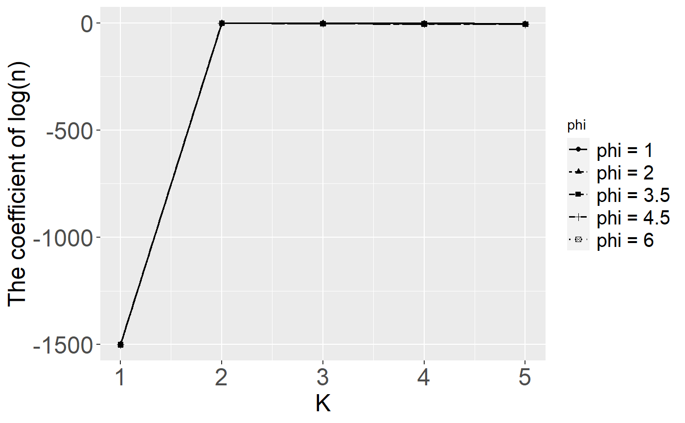
(a) $n=10^{4}$

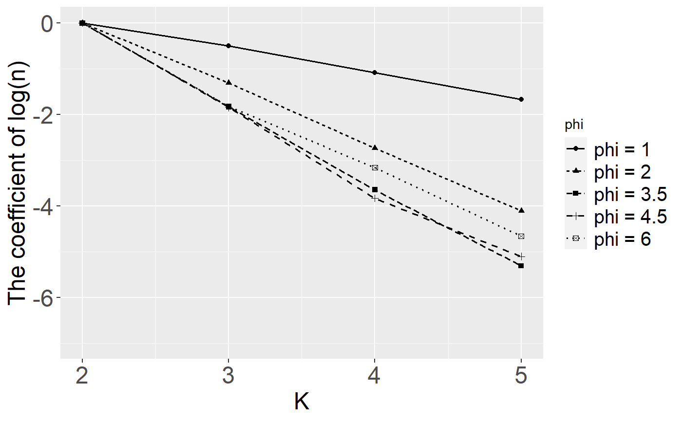
(b) $n=10^{4}$

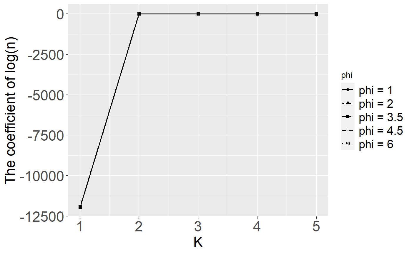
(c) $n=10^{5}$

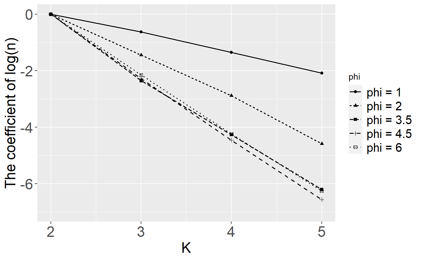
(d) $n=10^{5}$

Figure 1: Plots of $(\widehat{\mathcal{L}}_{K}-\widehat{\mathcal{L}}_{K^{*}})/\log n$ versus $K$ with fixed $n$.

4.1 Impact of $\phi_{0}$ on ELBO in finite mixture models

To study the effectiveness of using the ELBO $\mathcal{L}(\widehat{q}_{Z^{n}})$ analyzed in Theorem 2 for selecting the true number of components, and to examine how different choices of $\phi_{0}$ may impact the selection results, we conduct a numerical experiment using a location Gaussian mixture model under different settings. The ELBO is computed using the Coordinate Ascent Variational Inference (CAVI) algorithm (Bishop,, 2006). The simulated data $X^{n}=(X_{1},\ldots,X_{n})$ is generated from a $d$-dimensional Gaussian mixture model with $K^{*}=2$ components and $d=6$. We use a common variance-covariance matrix for the mixture components, which is the identity matrix $\bm{I}$ and treated as known. The true mixing weights are $w_{1}^{*}=w_{2}^{*}=1/2$ and the two true location parameters are $\eta_{1}^{*}=-2/\sqrt{d}\cdot\bf{1}$ and $\eta_{2}^{*}=2/\sqrt{d}\cdot\bf{1}$, where $\bf{1}$ denotes the $d$-dimensional all one vector. We employ a symmetric Dirichlet prior Diri$(\phi_{0},\ldots,\phi_{0})$ for the mixing weight $w$ and an independent $N(\bf{0},\,\bf{I})$ prior for the location parameters $\{\eta_{k}\}_{k=1}^{K}$. We consider $K_{\max}=5$ candidate Gaussian mixture models with component number $K\in\{1,2,\ldots,K_{\max}\}$. For our implementations, we found that the CAVI algorithm can be sensitive to the initialization of mixing weights $\overline{\bm{w}}$, especially in the regular regime when $\phi_{0}>(d+1)/2$. Therefore, in every simulation, the following initialization scheme is applied to enhance the computational stability: we randomly and evenly assign all data points $X^{n}$ into $K_{\rm int}$ groups at the beginning to initialize the latent class indicators $S^{n}$ for each $K_{\rm int}\in\{1,2,\ldots,K\}$, and then iteratively update $q_{S^{n}}(s^{n})$ and $q_{\theta}(\theta)$ until the ELBO value converges. For each $K$, we select the largest ELBO value obtained among different random initializations (i.e., under different $K_{\rm int}$) as our final output of $\mathcal{\widehat{L}}_{K}$, the ELBO value in the $K$ components mixture model.

In the first setting, we fix the sample size at $n\in\{10^{4},\,10^{5}\}$ and let $K$ and $\phi_{0}$ change. We choose $\phi_{0}\in\{1,2,3.5,4.5,6\}$, where $(d+1)/2=3.5$ corresponds to the critical threshold distinguishing the singular and regular regimes, as predicted in Theorem 2. In particular, our theory predicted that for $K>K^{*}$, the ELBO value $\widehat{\mathcal{L}}_{K}$ satisfies

$$\widehat{\mathcal{L}}_{K}-\widehat{\mathcal{L}}_{K^{*}}=\mathcal{O}_{P}(1)-\min\{\phi_{0},\,3.5\}\,(K-K^{*})\,\log n.$$ (13)

Consequently, when plotting $(\widehat{\mathcal{L}}_{K}-\widehat{\mathcal{L}}_{K^{*}})/\log n$ against $K$, the resulting curve will approximate a straight line with a slope of $-\min\{\phi_{0},\,3.5\}$. The numerical results shown in Figure 1 confirm this theoretical prediction. The two graphs on the left show the ELBO values overall considered $K$, while the two graphs on the right zoom in on the over-specified range of $K\geq K^{*}$. As we can see, for all cases, ELBO is maximized at the true model with $K=K^{*}=2$. Additionally, under a relatively small sample size, as in Figure 1(b), the slope under $\phi_{0}=6$ has a clear deviation from the theoretical value of $3.5$ based on equation (13); this situation improves under the relatively larger sample size, as in Figure 1(d). This observation can be explained by our discussion after Theorem 2, which suggests that using a large $\phi_{0}$ may not be a good choice for small sample sizes due to higher approximation errors $(C_{1},C_{2})$.

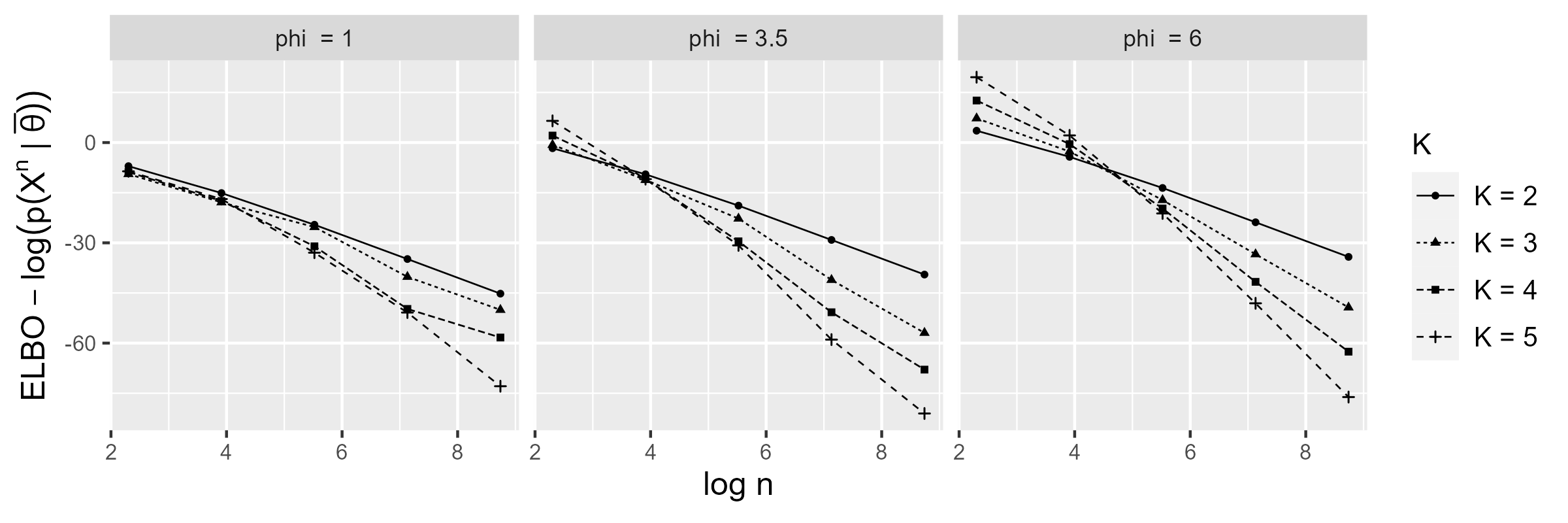
Figure 2: Plots of $\big{[}\widehat{\mathcal{L}}_{K}-\log p(X^{n}|\overline{\theta})\big{]}$ versus $\log n$ with fixed $\phi_{0}$.

To formally study the impact of $\phi_{0}$ on model selection, we consider a second setting where we fix $\phi_{0}$ and vary $n\in\{10,10\cdot 5,10\cdot 5^{2},10\cdot 5^{3},10\cdot 5^{4}\}$ and $K\in\{2,3,4,5\}$. Figure 2 reports the results, where we plot $\big{[}\widehat{\mathcal{L}}_{K}-\log p^{*}(X^{n})\big{]}$ against $\log n$ with a fixed $\phi_{0}\in\{1,3.5,6\}$. As can be seen from Figure 2, for $\phi_{0}=1$, the ELBO values $\widehat{\mathcal{L}}_{K}$ is already peaked at $K^{*}$ at a sample size as small as $n=10$. However, for $\phi_{0}=6$, a much larger sample size (around $e^{4.5}=90$) is required for the ELBO to peak at the true model with $K^{*}=2$. This empirical result again suggests that a smaller value of $\phi_{0}$ is preferred for accurate model selection with limited data.

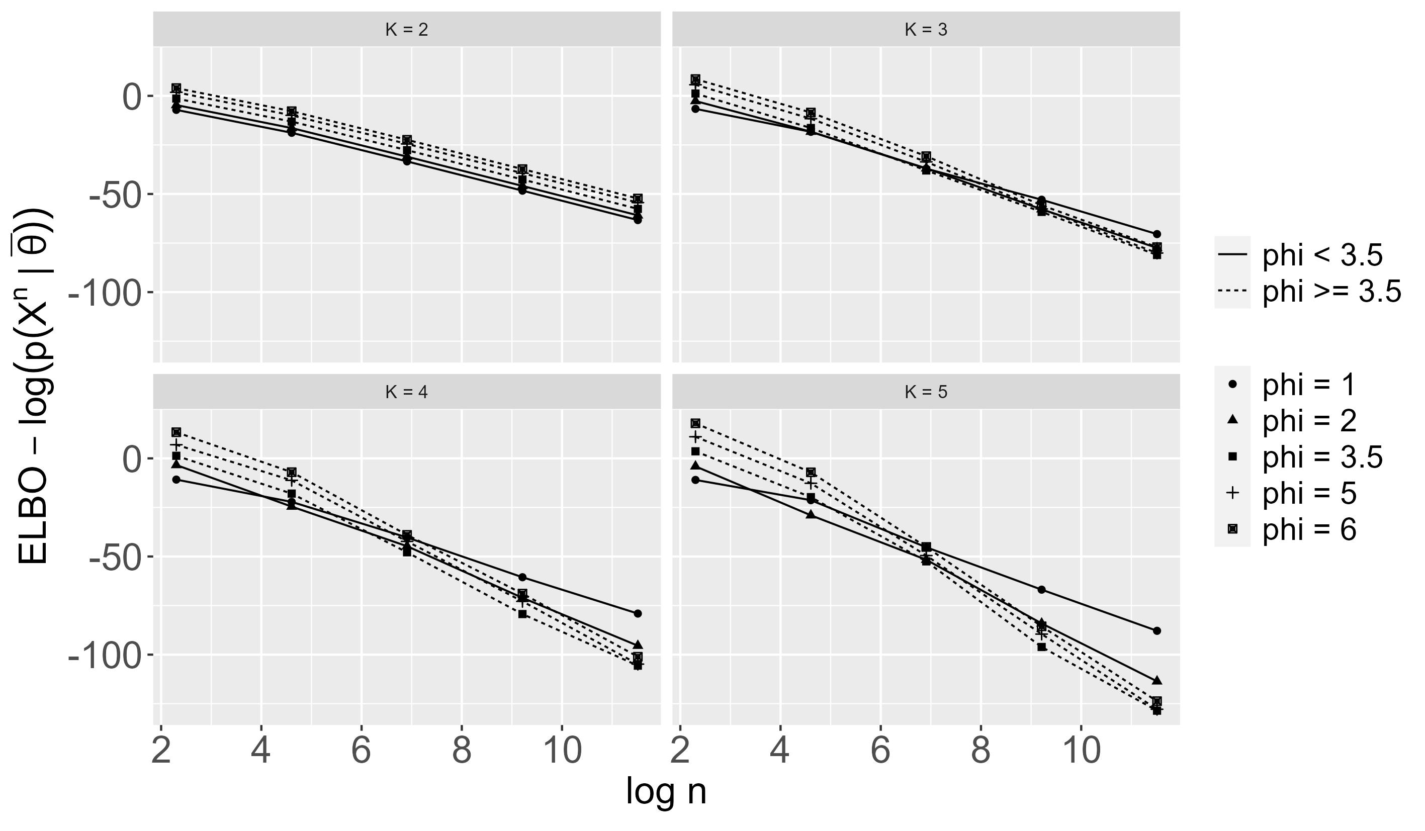
Figure 3: Plots of $(\widehat{\mathcal{L}}_{K}-\widehat{\mathcal{L}}_{K^{*}})/\log n$ versus $\phi_{0}$ with fixed $K$.

We also use the setting of a fixed $K$ and varied $n$ to numerically verify the theoretical dependence of the coefficients of $\log n$ in the ELBO on $\phi_{0}$. According to Theorem 2, if we plot $\mathcal{L}(\widehat{q}_{Z^{n}})-\log p(X^{n}|\overline{\theta})$ against $\log n$, we expect to see a linear relationship with a slope of $-\lambda$, which equals to $(K-K^{*})\phi_{0}+(dK^{*}+K^{*}-1)/2$ for $\phi_{0}<3.5$ and $(dK+K-1)/2$ for $\phi_{0}>3.5$. The corresponding results are summarized in Figure 3. As we can see, the slopes of the lines for larger $\phi_{0}=\{3.5,4.5,6\}$ exceeding the critical threshold $(d+1)/2=3.5$ remains essentially unchanged across different $K$. For $\phi_{0}<3.5$, the lines becomes less steep compared to $\phi=3.5$ as $K$ increases. Those empirical observations again align well with the prediction from our theory.

Finally, to examine the stability behavior of the variational approximation $\widehat{q}_{w}$ which tends to empty out the redundant mixture components under over-specified $K>K^{*}$, we conduct a last simulation study to report the variational point estimators of the mixing weights (expectations under $\widehat{q}_{w}$), denoted as $\overline{w}$, under $K=5$ and $K^{\ast}=2$. In Table 1, we report the (sorted) estimated weights $\overline{w}_{k}$’s for each setting. We repeated every setting ten times and recorded the means and standard deviations. The behavior of $\overline{w}_{k}$ is consistent with our predictions from Corollary 5: for small $\phi_{0}<3.5$, the mixing weights tend to only concentrate on the first two components; while for large $\phi>3.5$, the mixing weights tend to spread out over all $K=5$ mixture components. Moreover, for large $\phi\geq 3.5$, the estimated weights tend to be fairly sensitive to the initialization so the standard deviations are higher, which again suggests that a small $\phi_{0}$ should be used in order to enhance the parameter estimation robustness and accuracy. In addition, in Table 2 we report the estimated Wasserstein distances between the estimated mixing distribution $G(\overline{\theta})$ and the true mixing distribution $G^{*}$ to compare the convergence rate of component parameters. From the table, we can observe that the estimation errors in terms of $W_{1}(G(\overline{\theta}),G^{*})$ (and standard deviations) under both $n=1000$ and $n=10000$ are substantially smaller under a small $\phi_{0}<3.5$ (singular regime) compared to those under a large $\phi_{0}>3.5$ (regular regime).

			$\overline{w}_{1}$	$\overline{w}_{2}$	$\overline{w}_{3}$	$\overline{w}_{4}$	$\overline{w}_{5}$
$n=1000$	$\phi_{0}=1$	Mean	0.505	0.484	0.004	0.004	0.004
		Std	0.007	0.006	0.002	0.002	0.002
	$\phi_{0}=2$	Mean	0.490	0.461	0.017	0.017	0.017
		Std	0.008	0.013	0.002	0.002	0.002
	$\phi_{0}=3.5$	Mean	0.441	0.356	0.116	0.056	0.030
		Std	0.069	0.080	0.081	0.051	0.016
	$\phi_{0}=4.5$	Mean	0.392	0.298	0.155	0.104	0.051
		Std	0.057	0.058	0.039	0.037	0.029
	$\phi_{0}=6$	Mean	0.343	0.274	0.184	0.123	0.076
		Std	0.051	0.041	0.040	0.028	0.026
$n=10000$	$\phi_{0}=1$	Mean	0.503	0.495	$<$0.001	$<$0.001	$<$0.001
		Std	0.003	0.003	$<$0.001	$<$0.001	$<$0.001
	$\phi_{0}=2$	Mean	0.502	0.487	0.007	0.002	0.002
		Std	0.004	0.014	0.016	$<$0.001	$<$0.001
	$\phi_{0}=3.5$	Mean	0.464	0.418	0.078	0.027	0.023
		Std	0.080	0.100	0.103	0.053	0.032
	$\phi_{0}=4.5$	Mean	0.407	0.279	0.149	0.108	0.057
		Std	0.083	0.098	0.055	0.044	0.049
	$\phi_{0}=6$	Mean	0.384	0.272	0.158	0.109	0.078
		Std	0.076	0.079	0.053	0.046	0.037

Table 1: Estimated mixing weights $\{\overline{w}_{k}\}_{k=1}^{5}$ under $n\in\{10^{3},10^{4}\}$ and $\phi_{0}\in\{1,2,3.5,4.5,6\}$.

	$n=1000$					$n=10000$
$\phi_{0}$	1	2	3.5	4.5	6	1	2	3.5	4.5	6
Mean	0.151	0.222	0.341	0.414	0.422	0.048	0.057	0.098	0.157	0.169
Std	0.023	0.029	0.114	0.056	0.070	0.014	0.012	0.068	0.058	0.050

Table 2: Estimated $W_{1}(G(\overline{\theta}),G^{*})$ under $n\in\{10^{3},10^{4}\}$ and $\phi_{0}\in\{1,2,3.5,4.5,6\}$.

4.2 Comparison with other model selection methods

Recently, a method for model selection of finite mixture models (FMMs) named Group-Sort-Fuse (GSF) has been proposed by Manole and Khalili, (2021), which is shown to enjoy higher consistency and efficiency than existing approaches such as the Merge-Truncate-Merge (MTM) algorithm provided by Guha et al., (2021). Specifically, GSF is a penalized likelihood method to simultaneously estimate the number of components and the mixing measure $G(\theta)$. Three commonly used penalties, the Smoothly Clipped Absolute Deviation (SCAD), the Minimax Concave Penalty (MCP), and the Adaptive Lasso (ALasso), which meet the required theoretical conditions, are advocated in their paper. In Manole and Khalili, (2021), they already compared their method to the MTM algorithm, which has lower accuracy and incurs high computational costs since it is based on sampling from the real posterior distribution. Therefore, in this simulation study, we will only study and compare the three methods, ELBO (under $\phi=1$ and $\phi=5$), BIC, and GSF with the three different penalties (denoted as ${\rm GSF_{S}}$, ${\rm GSF_{M}}$ and ${\rm GSF_{A}}$) for selecting the number of components in a location Gaussian mixture model. For the model setting, we adopt a similar data-generating model as Manole and Khalili, (2021). Specifically, we consider the six mixture models as summarized in Table 3 (two within each group) in the Appendix B with true number of components $K^{*}=2,3,5$ and mixture component parameter dimensions $d=2,4,6$. The component parameters $\eta_{k}^{*}$ (location parameters) in Models 1, 3, and 5 are the same as those from Manole and Khalili, (2021), but we change the mixing weights $w^{*}=(w_{1}^{*},\ldots,w_{5}^{*})$ to be unevenly distributed. Models 2, 4, and 6 are less separated (i.e., with closer location parameters $\{\eta_{k}^{\ast}\}_{k=1}^{5}$), with the same component numbers and dimensions as in Models 1, 3, and 5, respectively. For each model, we assume the identity covariance matrix as known. We randomly generate the data $X^{n}$ 100 times with varying sample sizes $n=200,400,600,800$ for each model, then apply each method and record the model selection accuracy (percentages of selecting the correct model).

The findings are illustrated in Figure 4. A notable observation is that ELBO demonstrates superior performance compared to all other methods in scenarios where the separation between mixture components is relatively small (Models 2, 4, and 6). Particularly in Model 6, ELBO achieves an accuracy exceeding 0.875 with a sample size of 800, while alternative methods yield accuracies of 0. The tendency of other methods to select smaller models is attributed to the small (cluster) separation, often resulting in the selection of only one component. Moreover, in Models 3, and 5, where component weights are unevenly distributed, GSF exhibits suboptimal performance compared to the findings presented in (Manole and Khalili,, 2021), as GSF imposes a large penalty when some component weights approach zero, leading to model underestimation. Additionally, for ELBO, similar to our earlier results, larger values of $\phi_{0}$ (regular regime) yield lower accuracy compared to smaller $\phi_{0}$ (singular regime), especially when the sample size is small, as demonstrated in Model 2, 4, and 6. However, overall, even ELBO with a large $\phi_{0}$ still outperforms other methods. In summary, our simulation results for Gaussian mixture models indicate that ELBO generally outperforms GSF under the following conditions: (1) large number of components and parameter dimensions; (2) uneven distribution of mixing weights; and (3) similar mixture components or small cluster separations.

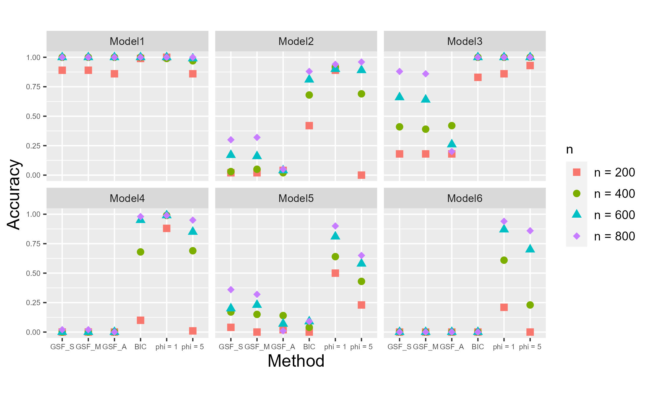
Figure 4: Percentages of selecting the correct model in the multivariate Gaussian mixture model.

4.3 ELBO and evidence

In this subsection, we empirically compare and calculate the difference between the ELBO and the true model evidence. Aoyagi, (2010) derived the real log canonical threshold (RLCT) for the univariate location Gaussian distribution. Note that the RLCT determines the (asymptotic) leading coefficient in front of $\log n$ for the true model evidence. The RLCT values in (3) are given as

$$\lambda_{\mathcal{M}}=K^{*}-1+\frac{j+j^{2}+2(K-K^{*}+1)}{4(j+1)}\ \ \mbox{with}\ \ j=\max\{i:\,i+i^{2}\leq 2(K-K^{*}+1)\}.$$

We visualize these metrics by plotting the ELBO, which includes the empirical evidence (denoted as ${\rm Evidence_{\rm E}}$) derived from MCMC sampling and the theoretical evidence (denoted as ${\rm Evidence_{\rm T}}$) by plugging-in the theoretical RLCT value; the data-generating model is $p^{*}(x)=\frac{1}{2}\mathcal{N}(-2,1)+\frac{1}{2}\mathcal{N}(2,1)$ with a sample size of $n=10000$. The empirical evidence is obtained via the Monte Carlo method using samples generated from the posterior distribution using a Metropolis-Hastings algorithm, with a Monte Carlo sample size of $N=20000$. From the results in Figure 6, we observe that the ELBO under a relatively small $\phi=1/4$ (singular regime) tends to be closer to both evidence values, while that under a relatively large $\phi=1$ (regular regime) resembles the BIC, which is consistent with our theoretical predictions. Moreover, despite the slight discrepancies between ELBO values and evidence values, they remain close and have the same overall trend as model size grows, ensuring that the ELBO inherits the consistency of model selection from using the true evidence.

4.4 Real Data Analysis

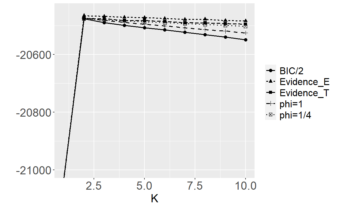
Figure 5: ELBO and true evidence values for Gaussian mixture model with $K$ components.

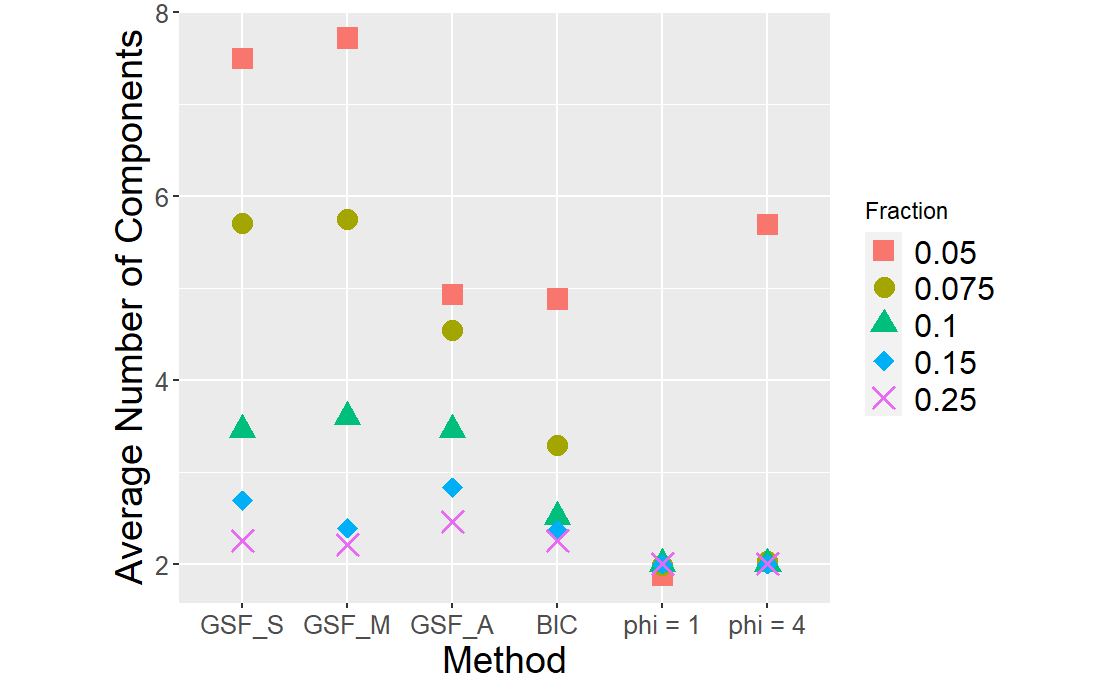
Figure 6: Selected component numbers with different fractions of the original data

In this subsection, we apply our method to the old Faithful geyser eruption data, which contains 272 two-dimensional data points. By examining the scatter plot (Section 4.2.2 in Ohn and Lin, (2023)), it appears that two components are sufficient to represent the data. We preprocess the data to equalize the variances of the two dimensions by dividing the waiting time by 15 and setting $\sigma^{2}=0.25$. We apply each method using 5%, 7.5%, 10%, 15%, and 25% of the entire dataset to determine the minimal sample size required for each method to correctly select the true number of components. For each fraction, we repeat the subsampling 100 times and report the averaged number of components selected by different methods. As shown in Figure 6, when $\phi_{0}=1$, the (averaged) number of components selected by the ELBO is already very close to 2 with just 14 data points (5% fraction) and remains unchanged when the fraction exceeds 7.5%. However, with $\phi_{0}=4$, a preference for a larger model (6 is the upper limit we set) is observed when the sample size is small. All three penalties of the GSF algorithm and the BIC show a trend toward correctly selecting the true number of components as the sample size increases. However, when the sample size is relatively small, BIC tends to incorrectly select an overly large model compared to the ELBO. This phenomenon could again be explained by the stability behavior of the ELBO (with a small $\phi$), which makes the variational posterior distribution under an overspecified model $\overline{\theta}$ more accurate than the maximum likelihood estimator $\widehat{\theta}$ (see Theorem 7 and Table 2), resulting in better power to distinguish true signals (i.e., separation between mixture components) from estimation errors due to a small size. A deterioration of the ELBO model selection performance observed in Figure 6 using a larger $\phi_{0}=4$ also empirically supports this explanation. A similar overestimation of the model size occurs with the three GSF methods, which could also be due to the same reason.

5 Discussion

In this paper, we advocate the use of ELBO from mean-field variational Bayes for model selection in finite mixture models. We analyze the large-sample properties of ELBO by proving matching lower and upper bounds that improve upon existing results by utilizing the consistency property of variational Bayes. As a direct consequence, we have established an asymptotic expansion for the ELBO and proved the consistency of model selection through ELBO maximization. As a by-product of our proof, we show that the stable behavior of the posterior distribution, which benefits from model singularity, can be inherited by the mean-field variational approximation to the posterior. We also derived a parametric convergence rate of $\log n/\sqrt{n}$ for component parameters.

As one future direction, we would like to extend the current development to other singular models such as hidden Markov models, neural networks, and factor models. Another future direction is to develop a finite sample analysis of the ELBO by providing a more refined characterization of the likelihood ratio test statistic under singularity, as we briefly commented after Corollary 5.

Supplementary Materials for “Model Selection for Finite Mixture Models via Variational Approximation”

Appendix A More Literature Review

In this appendix, we offer additional details on some of the literature reviewed in the main paper, along with information on several more related works.

Variational Bayes. Variational inference was introduced by Jordan et al., (1999) for probability density approximation with intractable integrals and point estimation for parameter determination. In variational inference, the posterior distribution is approximated by the closest member relative to the Kullback-Leibler (KL) divergence in a specified family. Among the various approximating schemes, mean-field approximation, where the variational family adopts a factorized form, emerges as the most prevalent type of variational inference. It is characterized by its conceptual simplicity, ease of implementation, and particular suitability for addressing problems that involve a high number of latent variables. Pati et al., (2018) relates the Bayes risk to the variational solution for a general distance metric. In addition, for non-singular models, which include finite mixture models with a known component number, Han and Yang, (2019) proved that the convergence rate of point estimators based on the variational posterior is $n^{-1/2}$, and they also provide the asymptotic normality of the optimal mean-field approximation centered at the maximum likelihood estimation.

Asymptotic properties of likelihood ratio tests in mixture models. The use of maximum likelihood estimator (MLE) for fitting mixture models has received a lot of attention from statisticians since the 1960s. Dempster et al., (1977) introduced a general iterative approach, the expectation–maximization (EM) algorithm, for computing the MLE in latent variable models. The convergence properties of the MLE for the mixture problem were then theoretically established. Meanwhile, the testing of homogeneity, in other words, determining whether the mixture model has only one component or more, became an important research question. For non-singular models, when under the null hypothesis the parameter is constrained in a subspace of the whole parameter space, the limit distribution of the likelihood ratio testing statistic (LRTS) $\Lambda_{n}$ is a chi-square distribution. Unlike in non-singular model testing, Hartigan, (1985) observed that under homogeneity, the statistic diverges to infinity if the whole parameter space is unrestricted. Ghosh and Sen, (1984) developed the asymptotic theory for the distribution of the LRTS under this setting. They showed that in the limit, $2\log\Lambda_{n}$ is distributed as the square of the supremum of a centered Gaussian process ${W_{S}:S\in\mathcal{S}}$ admitting continuous sample paths. Also, Bickel, (1993) investigated the null behavior of the LRTS for this model. At the beginning of the 21st century, more mixture models were considered, and the divergence rate of the LRTS with an unconstrained parameter space was verified. For example, normal mixture models in Liu and Shao, (2004) and gamma mixture models in Liu et al., (2003) were shown to diverge at the rate $\mathcal{O}(\log\log n)$. On the other hand, mixture models with restricted parameter spaces were also explored. While the limit distribution is still related to a Gaussian process, this time the index set $\mathcal{S}$ is compact, so the LRTS is bounded in probability. The general results for models with restricted parameter spaces under loss of identifiability are provided by Liu and Shao, (2003), and the application to finite mixture models can also be found in Section 4 of the same paper. Although their method may test the true model against the alternative, it requires prior knowledge about the true component number to set the null hypothesis, and the exact form of the Gaussian process still requires a case-by-case analysis.

Appendix B Table 3

Model	$w^{*}_{1},\eta^{*}_{1}$	$w^{*}_{2},\eta^{*}_{2}$	$w^{*}_{3},\eta^{*}_{3}$	$w^{*}_{4},\eta^{*}_{4}$	$w^{*}_{5},\eta^{*}_{5}$
1	0.3,$(0,0)^{T}$	0.7,$(2,2)^{T}$
2	0.5,$(\sqrt{2},0)^{T}$	0.5,$(0,\sqrt{2})^{T}$
3	0.2, $\left(\begin{matrix}0\\ 0\\ 0\\ 0\\ \end{matrix}\right)$	0.3, $\left(\begin{matrix}2.5\\ 1.5\\ 2\\ 1.5\\ \end{matrix}\right)$	0.5, $\left(\begin{matrix}1.5\\ 3\\ 2.75\\ 2\\ \end{matrix}\right)$
4	0.3, $\left(\begin{matrix}\sqrt{2}\\ 0\\ 0\\ 0\\ \end{matrix}\right)$	0.3, $\left(\begin{matrix}0\\ \sqrt{2}\\ 0\\ 0\\ \end{matrix}\right)$	0.4, $\left(\begin{matrix}0\\ 0\\ \sqrt{2}\\ 0\\ \end{matrix}\right)$
5	0.1, $\left(\begin{matrix}0\\ 0\\ 0\\ 0\\ 0\\ 0\\ \end{matrix}\right)$	0.3, $\left(\begin{matrix}-1.5\\ 2.25\\ -1\\ 0\\ 0.5\\ 0.75\\ \end{matrix}\right)$	0.1, $\left(\begin{matrix}0.25\\ 1.5\\ 0.75\\ 0.25\\ -0.5\\ -1\\ \end{matrix}\right)$	0.3,$\left(\begin{matrix}-0.25\\ 0.5\\ -2.5\\ 1.25\\ 0.75\\ 1.5\\ \end{matrix}\right)$	0.2, $\left(\begin{matrix}-1\\ -1.5\\ -0.25\\ 1.75\\ -0.5\\ 2\\ \end{matrix}\right)$
6	0.2, $\left(\begin{matrix}\sqrt{2}\\ 0\\ 0\\ 0\\ 0\\ 0\\ \end{matrix}\right)$	0.2, $\left(\begin{matrix}0\\ \sqrt{2}\\ 0\\ 0\\ 0\\ 0\\ \end{matrix}\right)$	0.2, $\left(\begin{matrix}0\\ 0\\ \sqrt{2}\\ 0\\ 0\\ 0\\ \end{matrix}\right)$	0.2, $\left(\begin{matrix}0\\ 0\\ 0\\ \sqrt{2}\\ 0\\ 0\\ \end{matrix}\right)$	0.2, $\left(\begin{matrix}0\\ 0\\ 0\\ 0\\ \sqrt{2}\\ 0\\ \end{matrix}\right)$

Table 3: Parameter settings for the multivariate Gaussian mixture models

Appendix C Proofs of Main Results

In this appendix, we collect all proofs of the theoretical results in the paper.

C.1 Proof of Lemma 8

Consider the two mixing distributions $G=\sum_{k=1}^{K}w_{k}\delta_{\eta_{k}}$ and $G^{*}=\sum_{k=1}^{K^{\ast}}w^{*}_{k}\delta_{\eta^{*}_{k}}$. Let $\delta:=\min_{j\neq k}|\eta^{*}_{j}-\eta^{*}_{k}|$ and $I_{k}^{\prime}:=\{j:|\eta_{j}-\eta_{k}^{*}|<\delta/2\}$ for $k\in[K^{*}]$, then $I_{k}^{\prime}$’s are disjoint by definition. Recall that $W_{r}^{r}(G,G^{*})=\inf_{q_{ij}}\sum_{i=1}^{K}\sum_{j=1}^{K^{*}}q_{ij}\big{|}\eta_{i}-\eta_{j}^{*}\big{|}^{r}$, where the infimum ranges over all $q_{ij}$ satisfying $\sum_{i\in[K]}q_{ij}=w^{*}_{j}$ and $\sum_{j\in[K^{*}]}q_{ij}=w_{i}$.

For each $k\in[K^{*}]$ and feasible $q_{ij}$, we will show

$$W_{r}^{r}(G,G^{*})\geq\Big{|}\sum_{i\in I_{k}^{\prime}}w_{i}-w_{k}^{*}\Big{|}\,\delta^{r}.$$ (14)

To see this, we consider two cases. In the first case when $\sum_{i\in I_{k}^{\prime}}w_{i}>w_{k}^{*}$, we have

$$W_{r}^{r}(G,G^{*}) \ \geq\inf_{q_{ij}}\sum_{i\in I_{k}^{\prime}}\sum_{j=1}^{K}q_{ij}\big{|}\eta_{i}-\eta_{j}^{*}\big{|}^{r}\geq\inf_{q_{ij}}\Big{(}\sum_{i\in I_{k}^{\prime}}q_{ik}\big{|}\eta_{i}-\eta_{k}^{*}\big{|}^{r}+\sum_{i\in I_{k}^{\prime}}\sum_{j\neq k}q_{ij}\big{|}\eta_{i}-\eta_{j}^{*}\big{|}^{r}\Big{)}$$

$$\ \geq 0+\inf_{q_{ij}}\sum_{i\in I_{k}^{\prime}}\sum_{j\neq k}q_{ij}(\delta/2)^{r}.$$ (15)

Since $\sum_{i\in I_{k}^{\prime}}\sum_{j\in[K^{*}]}q_{ij}=\sum_{i\in I_{k}^{\prime}}w_{i}$ and $\sum_{i\in I_{k}^{\prime}}q_{ik}\leq\sum_{i\in[K]}q_{ik}=w_{k}^{*}$ for all feasible $q_{ij}$, we obtain $\sum_{i\in I_{k}^{\prime}}\sum_{j\neq k}q_{ij}\geq\sum_{i\in I_{k}^{\prime}}w_{i}-w_{k}^{*}$. This inequality combined with (15) leads to bound (14). In the second case when $\sum_{i\in I_{k}^{\prime}}w_{i}\leq w_{k}^{*}$, we have

$$W_{r}^{r}(G,G^{*})\geq\inf_{q_{ij}}\sum_{i=1}^{K}q_{ik}\big{|}\eta_{i}-\eta_{k}^{*}\big{|}^{r}=\inf_{q_{ij}}\Bigg{(}\sum_{i\in I_{k}^{\prime}}q_{ik}\big{|}\eta_{i}-\eta^{*}_{k}\big{|}^{r}+\sum_{i\notin I_{k}^{\prime}}q_{ik}\big{|}\eta_{i}-\eta^{*}_{k}\big{|}^{r}\Bigg{)}.$$

Since $\sum_{i\in[K]}q_{ik}=w^{*}_{k}$ and $\sum_{i\in I_{k}^{\prime}}q_{ik}\leq\sum_{i\in I_{k}^{\prime}}\sum_{j\in[K^{*}]}q_{ij}=\sum_{i\in I_{k}^{\prime}}w_{i}$, we can obtain that $\sum_{i\notin I_{k}^{\prime}}q_{ik}\geq w_{k}^{*}-\sum_{i\in I_{k}^{\prime}}w_{i}$, which further implies bound (14) due to the preceding display and the definition of $I_{k}$.

Finally, since $K^{*}$ is finite, we obtain from inequality (14) that

$$W_{r}^{r}(G,G^{*}) \geq(K^{*})^{-1}\sum_{k=1}^{K^{*}}\Big{|}\sum_{i\in I_{k}^{\prime}}w_{j}-w_{k}^{*}\Big{|}\,\delta^{r}$$

$$\gtrsim\sum_{k=1}^{K^{*}}\Big{|}\sum_{i\in I_{k}^{\prime}}w_{j}-w_{k}^{*}\Big{|}\,\delta^{r}\geq\inf_{I_{1},...,I_{K^{*}}}\sum_{k=1}^{K^{*}}\Big{|}\sum_{i\in I_{k}}w_{j}-w_{k}^{*}\Big{|}\,\delta^{r}.$$ (16)

The claimed bound then follows by combing above with inequality (11).

C.2 Proof of Theorem 2

The proof is divided into three steps. Firstly, we decompose the ELBO into two parts and obtain some analytically manageable approximations to both parts. Secondly, we constructively prove the claimed lower bound by using two instances of $q_{Z^{n}}$, since for any $q_{Z^{n}}$, $L(q_{Z^{n}})$ provides a lower bound to the ELBO. Finally, we prove the claimed upper bound based on the key Lemma 9 and our Assumption A2.

Step 1: For the complete-data $\{X^{n},S^{n}\}$, we denote the posterior probability of $X_{i}$ coming from the $k\,$th component as $\widehat{p}_{ik}=\widehat{q}_{S^{n}}(S_{i}=k)$, and let $\widehat{n}_{k}=\sum_{i=1}^{n}\widehat{p}_{ik}$. Then according to formula (8), the variational posterior distribution $\widehat{q}_{\theta}(\theta)=\widehat{q}_{\bm{w}}(\bm{w})\otimes\widehat{q}_{\bm{\eta}}(\bm{\eta})$ can be written as

$$\widehat{q}_{\bm{w}}(\bm{w})=\frac{\Gamma(n+K\phi_{0})}{\prod^{K}_{k=1}\Gamma(\widehat{n}_{k}+\phi_{0})}\prod^{K}_{k=1}w_{k}^{(\widehat{n}_{k}+\phi_{0})-1},$$ (17)

and

$$\widehat{q}_{\bm{\eta}}(\bm{\eta})\propto\prod^{K}_{k=1}\pi(\eta_{k})\exp\left[\sum_{i=1}^{n}\widehat{p}_{ik}\left(\eta_{k}^{T}T(x_{i})-T_{0}(x_{i})-A(\eta_{k})\right)\right].$$ (18)

From equations (17) and (18), we observe that $\widehat{q}_{w}(w)$ and $\widehat{q}_{\eta}(\eta)$ are parameterized by (in other words, only depend on) $\{\widehat{p}_{ik}:\,i\in[n],k\in[K]\}$. Additionally, $\widehat{q}_{S^{n}}(s^{n})$ is also paramaterized by $\{\widehat{p}_{ik}\}$ due to formula (9). Therefore, we only need to analyze those $q_{\theta}(\theta)=q_{w}(w)\otimes q_{\eta}(\eta)$ taking the form of

$${q}_{\bm{w}}(\bm{w})=\frac{\Gamma(n+K\phi_{0})}{\prod^{K}_{k=1}\Gamma(n_{k}+\phi_{0})}\prod^{K}_{k=1}w_{k}^{(n_{k}+\phi_{0})-1},$$ (19)

and

$${q}_{\bm{\eta}}(\bm{\eta})\propto\prod^{K}_{k=1}\pi(\eta_{k})\exp\left[\sum_{i=1}^{n}p_{ik}\left(\eta_{k}^{T}T(X_{i})-T_{0}(X_{i})-A(\eta_{k})\right)\right].$$ (20)

where $n_{k}=\sum_{i=1}^{n}p_{ik}$; and given a $q_{\theta}(\theta)$, the optimal $q_{S^{n}}(s^{n})$ takes the following form with a normalization constant $C_{Q}$ (also parameterized by $\{p_{ik}\}$),

$${q}_{S^{n}}(s^{n})=\frac{1}{C_{Q}}\exp\left\{\int{{q}_{\theta}(\theta)}\log p(X^{n},s^{n}\,|\,\theta)d\theta\right\}.$$ (21)

In the rest of the proof, we only consider those $q_{\bm{w}}(\bm{w})$, $q_{\bm{\eta}}(\bm{\eta})$ and $q_{S^{n}}(s^{n})$ having the forms as (19), (20) and (21). Based on these characterizations, we know that maximizing $\mathcal{L}(q_{Z^{n}})$ over $q_{Z^{n}}(z^{n})=q_{\theta}(\theta)\otimes q_{S^{n}}(S^{n})$ is equivalent to maximizing $\mathcal{L}(q_{Z^{n}})$ over all possible combinations of $\{p_{ik}:\,i\in[n],k\in[K]\}$ subject to $0\leq p_{ik}\leq 1$ and $\sum_{k=1}^{K}p_{ik}=1$ for all $i$.

We now characterize the ELBO function. According to the definition of $\mathcal{L}(q_{Z^{n}})$ in (5), we can decompose the ELBO into two parts as

$$\mathcal{L}(q_{Z^{n}}) \ =\int q_{Z^{n}}(z^{n})\log\frac{p(X^{n},s^{n}\,|\,\theta)\pi(\theta)}{q_{Z^{n}}(z^{n})}dz^{n}$$

$$\ =\int q_{\theta}(\theta)\log\frac{\pi(\theta)}{q_{\theta}(\theta)}d\theta+\sum_{s^{n}}q_{S^{n}}(s^{n})\int q_{\theta}(\theta)\log\frac{p(X^{n},s^{n}\,|\,\theta)}{q_{S^{n}}(s^{n})}d\theta,$$

where the first part is just $-D_{\rm KL}({q}_{\theta}(\theta)\|\pi(\theta))$ and the second term is $\log C_{Q}$. Then we can reformulate $\mathcal{L}(\widehat{q}_{Z^{n}})$ as

$$\mathcal{L}(\widehat{q}_{Z^{n}})=\max_{\{p_{ik}\}}\Big{\{}-D_{\rm KL}(q_{\theta}(\theta)\|\pi(\theta))+\log C_{Q}\Big{\}}.$$ (22)

We consider the KL divergence part first. Recall that priors on $w$ and $\eta$ are independent, which leads to

$$D_{\rm KL}({q}_{\theta}(\theta)\|\pi(\theta))=D_{\rm KL}({q}_{\bm{w}}(\bm{w})\|\pi(\bm{w}))+D_{\rm KL}({q}_{\bm{\eta}}(\bm{\eta})\|\pi(\bm{\eta})).$$

For the $D_{\rm KL}({q}_{\bm{w}}(\bm{w})\|\pi(\bm{w}))$ term, we can use the closed forms of the prior and the variational posterior of $w$ to explicitly calculate

$$\int{q}_{\bm{w}}(\bm{w})\log w_{k}dw=\Psi(n_{k}+\phi_{0})-\Psi(n+K\phi_{0}),$$ (23)

where $\Psi(x)=\Gamma^{\prime}(x)/\Gamma(x)$ is the so-called di-gamma function. This further leads to

$$D_{\rm KL}({q}_{\bm{w}}(\bm{w})\|\pi(\bm{w}))=\sum^{K}_{k=1}(n_{k}\Psi(n_{k}+ \ \phi_{0})-\log\Gamma(n_{k}+\phi_{0}))-n\Psi(n+K\phi_{0})$$

$$\ +\log\Gamma(n+K\phi_{0})+\log\frac{\Gamma(\phi_{0})^{K}}{\Gamma(K\phi_{0})},$$ (24)

where the last term causes the undesirable behavior under large $\phi_{0}$ as discussed after Theorem 2. To further simplify this expression, we resort to the following two inequalities: for any $x>0$ (Alzer,, 1997), we have

$$\frac{1}{2x}<\log x-\Psi(x)<\frac{1}{x},$$ (25)

and

$$0\leq\log\Gamma(x)-\left((x-\frac{1}{2})\log x-x+\frac{1}{2}\log 2\pi\right)\leq\frac{1}{12x}.$$

Applying these two inequalities to (24), we can obtain

$$\Big{|}D_{\rm KL}({q}_{\bm{w}}(\bm{w})\|\pi(\bm{w}))-(K\phi_{0}-\frac{1}{2})\log n+(\phi_{0}-\frac{1}{2})\sum_{k=1}^{K}\log(n_{k}+\phi_{0})\Big{|}<C,$$ (26)

for some constant $C$ independent of $n$ and $\phi_{0}$.

As to the $D_{\rm KL}({q}_{\eta}(\eta)\|\pi(\eta))$ term, since both the prior $\pi$ and the variational posterior of $\eta_{k}$ are factorized under our setup, we have

$$D_{\rm KL}({q}_{\bm{\eta}}(\bm{\eta})\|\pi(\bm{\eta}))=\sum_{k=1}^{K}D_{\rm KL}({q}_{\eta_{k}}(\eta_{k})\|\pi(\eta_{k})).$$

For each fixed $k\in[K]$, we denote the variational posterior mode (i.e., maximizer of its density function) as

$$\widehat{\eta}_{k}=\mathop{\arg\max}\limits_{\eta_{k}}\ \underbrace{\sum_{i=1}^{n}p_{ik}\left(\eta_{k}^{T}T(x_{i})+T_{0}(x_{i})-A(\eta_{k})\right)}_{\ell_{nk}(\eta_{k})},$$ (27)

Note that the critical point $\widehat{\eta}_{k}$ satisfies the first order condition $\nabla_{\eta_{k}}\ell_{nk}(\widehat{\eta}_{k})=0$. Under this notation, we can decompose $D_{\rm KL}({q}_{\eta_{k}}(\eta_{k})\|\pi(\eta_{k}))$ as

$$D_{\rm KL}(q_{\eta_{k}}(\eta_{k})\|\pi(\eta_{k})) \ =\int q_{\eta_{k}}(\eta_{k})\log\frac{q_{\eta_{k}}(\eta_{k})}{\pi(\eta_{k})}$$

$$\ =\int q_{\eta_{k}}(\eta_{k})\log\frac{\pi(\eta_{k})\exp\{\ell_{nk}(\eta_{k})-\ell_{nk}(\widehat{\eta}_{k})\}}{\pi(\eta_{k})\int\pi(\eta_{k})\exp\{\ell_{nk}(\eta_{k})-\ell_{nk}(\widehat{\eta}_{k})\}d\eta_{k}}$$

$$\ =\int q_{\eta_{k}}(\eta_{k})\left(\ell_{nk}(\eta_{k})-\ell_{nk}(\widehat{\eta}_{k})\right)d\eta_{k}$$

$$\ \qquad-\log\int\pi(\eta_{k})\exp\{\ell_{nk}(\eta_{k})-\ell_{nk}(\widehat{\eta}_{k})\}d\eta_{k}.$$ (28)

For the second term, applying Taylor expansion of $\ell_{nk}(\eta_{k})$ at $\widehat{\eta}_{k}$ up to the second order, we obtain

$$\ell_{nk}(\eta_{k})-\ell_{nk}(\widehat{\eta}_{k})=-\frac{1}{2}\sum_{i=1}^{n}p_{ik}(\eta_{k}-{\widehat{\eta}}_{k})^{T}I(\widetilde{\eta}_{ik})\,(\eta_{k}-\widehat{\eta}_{k}),$$

where $\widetilde{\eta}_{ik}$ lies on the segment between $\eta_{k}$ and $\widehat{\eta}_{k}$ such that $\widetilde{\eta}_{ik}=\widehat{\eta}_{k}+t_{i}(\eta_{k}-\widehat{\eta}_{k}),t_{i}\in[0,1]$. Then a standard Laplace’s approximation for integrals, e.g., equation (6.4.35) in Bender and Orszag, (2013), implies that with $n_{k}$ large enough, the second integral in (28) satisfies

$$\left|\frac{\int\pi(\eta_{k})\exp\{\ell_{nk}(\eta_{k})-\ell_{nk}(\widehat{\eta}_{k})\}d\eta_{k}}{(2\pi/n_{k})^{\frac{d}{2}}}-\frac{\pi(\widehat{\eta}_{k})}{\sqrt{I(\widehat{\eta}_{k})}}\right|\leq\frac{C}{n_{k}}.$$ (29)

Therefore, for large $n_{k}$, we have

$$\left|-\log\int\pi(\eta_{k})\exp\{\ell_{nk}(\eta_{k})-\ell_{nk}(\widehat{\eta}_{k})\}d\eta_{k}+\frac{d}{2}\log n_{k}\right|\leq C.$$ (30)

For the first term, by plugging in the explicit form of $q(\eta)$ from (20) into the integral, we obtain

$$\int q_{\eta_{k}}(\eta_{k})\left(\ell_{nk}(\eta_{k})-\ell_{nk}(\widehat{\eta}_{k})\right)d\eta_{k}= \ \frac{\int\pi(\eta_{k})\left(\ell_{nk}(\eta_{k})-\ell_{nk}(\widehat{\eta}_{k})\right)\exp\{\ell_{nk}(\eta_{k})-\ell_{nk}(\widehat{\eta}_{k})\}d\eta_{k}}{\int\pi(\eta_{k})\exp\{\ell_{nk}(\eta_{k})-\ell_{nk}(\widehat{\eta}_{k})\}d\eta_{k}},$$

whose denominator is already analyzed. Using Laplace’s approximation again to the numerator, as well as the fact that the value of the integrand at $\widehat{\eta}_{k}$ vanishes, we obtain

$$\left|\frac{\int\pi(\eta_{k})\left(\ell_{nk}(\eta_{k})-\ell_{nk}(\widehat{\eta}_{k})\right)\exp\{\ell_{nk}(\eta_{k})-\ell_{nk}(\widehat{\eta}_{k})\}d\eta_{k}}{(2\pi/n_{k})^{\frac{d}{2}}}-0\right|\leq\frac{C}{n_{k}}.$$

Therefore, by noticing $\ell_{nk}(\eta_{k})\leq\ell_{nk}(\widehat{\eta}_{k})$, we have

$$-\frac{C}{n_{k}}\leq\int q_{\eta_{k}}(\eta_{k})\left(\ell_{nk}(\eta_{k})-\ell_{nk}(\widehat{\eta}_{k})\right)d\eta_{k}\leq 0.$$ (31)

Combining (28), (30) and (31) together, we finally obtain that for any sufficiently large $n_{k}$,

$$\Big{|}D_{\rm KL}(q_{\eta_{k}}(\eta_{k})\|\pi(\eta_{k}))-\frac{d}{2}\log n_{k}\Big{|}\leq C.$$ (32)

Step 2: Next we prove a lower bound for $\mathcal{L}(\widehat{q}_{Z^{n}})$. According to the characterization of ELBO in (22), every instance of $\{p_{ik}\}$ gives a lower bound to $\mathcal{L}(\widehat{q}_{Z^{n}})$. Let us consider the following two special constructions:

Construction (I): This construction applies to the case when $\phi_{0}>(d+1)/2$. For $1\leq k\leq K^{*}-1$, we can always choose $\{p_{ik}:\,i\in[n],k\in[K^{*}-1]\}$ such that

$$n_{k}=\sum_{i=1}^{n}p_{ik}=w_{k}^{*}(n+K\phi_{0}) \,-\phi_{0},\text{ i.e. }\frac{n_{k}+\phi_{0}}{n+K\phi_{0}}=w_{k}^{*},$$

$$\mbox{and}\ \ \sum_{i=1}^{n}p_{ik}T(x_{i})=n_{k}\nabla_{\eta_{k}} A(\eta_{k}^{*}),\text{ i.e. }\widehat{\eta}_{k}=\eta^{*}_{k},$$

and for $K^{*}\leq k\leq K$, we choose $\{p_{ik}:\,i\in[n],K^{*}\leq k\leq K\}$ such that

$$n_{k}=w^{*}_{K^{*}}\frac{n+K\phi_{0}}{K-K^{*}+1}-\phi_{0},\text{ i.e. } \,\frac{(n_{k}+\phi_{0})(K-K^{*}+1)}{n+K\phi_{0}}=w_{K^{*}}^{*}$$

$$\mbox{and}\ \ \sum_{i=1}^{n}p_{ik}T(x_{i})=n_{k}\nabla_{\eta_{k}} A(\eta_{K^{*}}^{*}),\text{ i.e. }\widehat{\eta}_{k}=\eta^{*}_{K^{*}}.$$

With this construction, all $n_{k}$’s are proportional to $n$, so we have from (32) that

$$D_{\rm KL}(q_{\bm{\eta}}(\bm{\eta})\|\pi(\bm{\eta}))\leq\frac{d}{2}\sum_{k=1}^{K}\log n_{k}+C.$$

Combining the above with the approximation (26) to $D_{\rm KL}(q_{\bm{w}}(\bm{w})\|\pi(\bm{w}))$, we have the following upper bound to the KL divergence between $q_{\theta}(\theta)$ and $\pi(\theta)$,

$$D_{\rm KL}(q_{\theta}(\theta)\|\pi(\theta)) \ \leq(K\phi_{0}-\frac{1}{2})\log n+\frac{d}{2}\sum_{k=1}^{K}\log n_{k}+(\frac{1}{2}-\phi_{0})\sum_{k=1}^{K}\log(n_{k}+\phi_{0})+C$$

$$\ \leq(K\phi_{0}-\frac{1}{2})\log n+(\frac{d+1}{2}-\phi_{0})\sum_{k=1}^{K}\log n_{k}+C$$

$$\ =(K\phi_{0}-\frac{1}{2})\log n+(\frac{d+1}{2}-\phi_{0})K\log n+C$$

$$\ =\frac{dK+K-1}{2}\log n+C.$$ (33)

As for the lower bound of $\log C_{Q}$, we can first rewrite $C_{Q}$ as

$$C_{Q} \ =\prod_{i=1}^{n}\sum_{s_{i}}\exp\int{q}_{\theta}(\theta)\log p(x_{i},s_{i}|\theta)d\theta$$

$$\ =\prod_{i=1}^{n}\sum_{k=1}^{K}\exp\left(\int{q}_{w_{k}}(w_{k})\log w_{k}dw_{k}+\int{q}_{\eta_{k}}(\eta_{k})\log g(x_{i};\eta_{k})d\eta_{k}\right).$$ (34)

Using equations (23) and (25) again, we obtain

$$\int{q}_{w_{k}}(w_{k})\log w_{k}dw_{k}=\Psi(n_{k}+\phi_{0})-\Psi(n+K\phi_{0})\geq\log\frac{n_{k}+\phi_{0}}{n+K\phi_{0}}-\frac{1}{n_{k}+\phi_{0}}.$$

Additionally, since $\eta_{k}^{*}=\widehat{\eta}_{k}$ in this construction, we can apply a Taylor expansion at $\eta_{k}^{*}$. Concretely, we can write $q_{\eta_{k}}(\eta_{k})$ explicitly according to (20) as,

$$\int{q}_{\eta_{k}}(\eta_{k})\log g(x_{i};\eta_{k})d\eta_{k} \ =\frac{\int\pi(\eta_{k})\log g(x_{i};\eta_{k})\exp\{\ell_{nk}(\eta_{k})-\ell_{nk}(\eta_{k}^{*})\}d\eta_{k}}{\int\pi(\eta_{k})\exp\{\ell_{nk}(\eta_{k})-\ell_{nk}(\eta_{k}^{*})\}d\eta_{k}}.$$

Under Assumption A1 and using the fact that $n_{k}\asymp n$, we can apply Laplace’s approximation to approximate the numerator and denominator respectively as,

$$\left|\frac{\int\pi(\eta_{k})\log g(x_{i};\eta_{k})\exp\{\ell_{nk}(\eta_{k})-\ell_{nk}(\eta_{k}^{*})\}d\eta_{k}}{(2\pi/n_{k})^{\frac{d}{2}}}\cdot\frac{\sqrt{I(\eta_{k}^{*})}}{\pi(\eta_{k}^{*})\log g(x_{i};\eta_{k}^{*})}-1\right|\leq\frac{C}{n_{k}},$$ (35)

and

$$\left|\frac{\int\pi(\eta_{k})\exp\{\ell_{nk}(\eta_{k})-\ell_{nk}(\eta_{k}^{*})\}d\eta_{k}}{(2\pi/n_{k})^{\frac{d}{2}}}\cdot\frac{\sqrt{I(\eta_{k}^{*})}}{\pi(\eta_{k}^{*})}-1\right|\leq\frac{C}{n_{k}}.$$ (36)

Therefore, with the choice of $w_{k}^{*}=(n_{k}+\phi_{0})/(n+K\phi_{0})$ for all $k<K^{*}$, we have

$$\ \sum_{k=1}^{K^{*}-1}\exp\left(\int{q}_{w_{k}}(w_{k})\log w_{k}dw_{k}+\int{q}_{\eta_{k}}(\eta_{k})\log g(x_{i};\eta_{k})d\eta_{k}\right)$$

$$\geq \ \sum_{k=1}^{K^{*}-1}\exp\left(\log w_{k}^{*}-\frac{1}{n_{k}+\phi_{0}}+\log g(x_{i};\eta_{k}^{*})-\log\left(1+\frac{C}{n_{k}}\right)\right)$$

$$\geq \ \sum_{k=1}^{K^{*}-1}w_{k}^{*}g(x_{i};\eta_{k}^{*})\left(1-\frac{C}{n}\right).$$

The same argument can applies to $k\geq K^{*}$, where by using the fact that $n_{k}\asymp n$, we can obtain that for all $K\geq K^{*}$,

$$\ \sum_{k=K^{*}}^{K}\exp\left(\int{q}_{w_{k}}(w_{k})\log w_{k}dw_{k}+\int{q}_{\eta_{k}}(\eta_{k})\log g(x_{i};\eta_{k})d\eta_{k}\right)$$

$$\geq \ \sum_{k=K^{*}}^{K}\exp\left(\log\frac{w_{K^{*}}^{*}}{K-K^{*}+1}-\frac{1}{n_{k}+\phi_{0}}+\log g(x_{i};\eta_{K^{*}}^{*})-\log\left(1+\frac{C}{n_{k}}\right)\right)$$

$$\geq \ w_{K^{*}}^{*}g(x_{i};\eta_{K^{*}}^{*})\left(1-\frac{C}{n}\right).$$

According to (34), the constant $\log C_{Q}$ can be bounded from below by

$$\log C_{Q}\geq\sum_{i=1}^{n}\log\left(\sum_{k=1}^{K^{*}}w_{k}^{*}g(x_{i};\eta_{k}^{*})\left(1-\frac{C}{n}\right)\right)=\log p^{*}(X^{n})-C.$$ (37)

Finally, by noticing the formulation of $\mathcal{L}(\widehat{q}_{Z^{n}})$ as in (22), we can add (33) and (37) together to get a lower bound when $\phi_{0}>(d+1)/2$ as

$$\mathcal{L}(\widehat{q}_{Z^{n}})-\log p^{*}(X^{n})\geq-\frac{dK+K-1}{2}\log n-C.$$ (38)

Construction (II): This construction applies to the case when $\phi_{0}\leq(d+1)/2$. For each $k$ such that $1\leq k\leq K^{*}$, we can always choose $\{p_{ik}:\,i\in[n],k\in[K^{*}]\}$ such that

$$n_{k}=\sum_{i=1}^{n}p_{ik}=w_{k}^{*}(n+\phi_{0}) -\phi_{0},\ \ \text{ i.e. }\frac{n_{k}+\phi_{0}}{n+K\phi_{0}}=w_{k}^{*},$$

$$\mbox{and}\ \ \sum_{i=1}^{n}p_{ik}T(x_{i}) =n_{k}\nabla_{\eta_{k}}A(\eta_{k}^{*});$$

and for $K^{*}<k\leq K$, we set $n_{k}=0$. Then for each $k>K^{*}$, $q_{\eta_{k}}(\eta_{k})$ is the same as prior density $\pi(\eta_{k})$, so we have $D_{\rm KL}(q_{\eta_{k}}(\eta_{k})\|\pi(\eta_{k}))=0$ for all $k>K^{*}$. For each $k\leq K^{*}$, we have $n_{k}\asymp n$, so (32) leads to

$$D_{\rm KL}(q_{\bm{\eta}}(\bm{\eta})\|\pi(\bm{\eta}))\leq\sum_{k=1}^{K^{*}}\frac{d}{2}\log n_{k}+C.$$

Combining the preceding display with (26), we obtain

$$D_{\rm KL}(q_{\theta}(\theta)\|\pi(\theta))\leq\left(\frac{dK^{*}+K^{*}-1}{2}+(K-K^{*})\phi_{0}\right)\log n+C.$$ (39)

Now since the summation over $k\in[K]$ for the $C_{Q}$ in (34) is dominated by its first $K^{*}$ terms, we can lower bound this summation to the sum of the first $K^{*}$ terms. Now, since $n_{k}\asymp n$ for $k\leq K^{*}$, we can apply (35) and (36) to obtain

$$\sum_{k=1}^{K^{*}}\exp\left(\int q_{\theta_{k}}(\theta_{k})\log\left(w_{k}g(x_{i};\eta_{k})\right)d\theta_{k}\right)\geq \ \sum_{k=1}^{K^{*}}w_{k}^{*}g(x_{i};\eta^{*}_{k})\left(1-\frac{C}{n}\right).$$

Putting all the pieces together, we obtain

$$\log C_{Q}\geq\sum_{i=1}^{n}\log\left(\sum_{k=1}^{K^{*}}w^{*}_{k}g(x_{i};\eta^{*}_{k})\right)+n\log\left(1-\frac{C}{n}\right)=\log p^{*}(X^{n})-C+\mathcal{O}\left(\frac{1}{n}\right).$$ (40)

Adding (39) and (40) together, we can obtain a lower bound to $\mathcal{L}(q_{Z^{n}}(z^{n}))$ for all $\phi_{0}\leq(d+1)/2$ as

$$\mathcal{L}(\widehat{q}_{Z^{n}})-\log p^{*}(X^{n})\geq-\left(\frac{dK^{*}+K^{*}-1}{2}+(K-K^{*})\phi_{0}\right)\log n-C.$$ (41)

Finally, combining (38) and (41) leads to the claimed lower bound of $\mathcal{L}(\widehat{q}_{Z^{n}})$.

Step 3: Now we derive an upper bound of the ELBO in (22). We first tackle the $\log\widehat{C}_{Q}$ term, recall that $\widehat{C}_{Q}$ is the normalization constant for the optimal distribution $\widehat{q}_{S^{n}}(s^{n})$ in (9). Note that $\log w_{k}$ is concave with respect to $w_{k}$. For $\log g(x;\eta_{k})$, the second order derivative with respect to $\eta_{K}$ is the negative fisher information matrix for the mixture component

$$\nabla^{2}_{\eta_{k}}\log g(x;\eta_{k})=-\nabla^{2}_{\eta_{k}}A(\eta_{k})=-I(\eta_{k}),$$

which is negative definite according to Assumption A1. Therefore, $\log g(x;\eta)$ is concave with respect to $\eta_{k}$. By applying Jensen’s inequality, we can then obtain

$$\int\widehat{q}_{w_{k}}(w_{k})\log w_{k}\,dw_{k}+\int\widehat{q}_{\eta_{k}}(\eta_{k})\log g(x;\eta_{k})\,d\eta_{k}\leq\log(\overline{w}_{k}g(x;\overline{\eta}_{k})),$$

which combined with (34) leads to

$$\log\widehat{C}_{Q}\leq\sum_{i=1}^{n}\log\left(\sum_{k=1}^{K}\overline{w}_{k}g(x_{i};\overline{\eta}_{k})\right)=\log p(X^{n}\,|\,\overline{\theta}).$$ (42)

The KL divergence $D_{\rm KL}(q_{w}(w)\|\pi(w))$ is the same as (26). As to the $D_{\rm KL}(q_{\eta}(\eta)\|\pi(\eta))$ term, note that for a large $n_{k}$, we can apply the approximation (32). Consequently, we define a set $\widehat{\mathcal{F}}:=\{k\,|\,1\leq k\leq K,\widehat{n}_{k}\geq M\}$, where $M$ is a sufficiently large (truncating) constant, to select those indices $k$ for which the approximation is accurate. This approximation, when combined with the non-negativity of the KL divergence, gives

$$D_{\rm KL}(\widehat{q}_{\bm{\eta}}(\bm{\eta})\|\pi(\bm{\eta}))=\sum_{k=1}^{K}D_{\rm KL}(\widehat{q}_{\eta_{k}}(\eta_{k})\|\pi(\eta_{k}))\geq\frac{d}{2}\sum_{k\in\mathcal{F}}\log\widehat{n}_{k}-C.$$

Using approximation (26) again, we can bound the entire KL divergence term from below as

$$D_{\rm KL}(\widehat{q}_{\theta}(\theta)\|\pi(\theta)) \ \geq(K\phi_{0}-\frac{1}{2})\log n+\left(\frac{d+1}{2}-\phi_{0}\right)\sum_{k\in\mathcal{F}}\log\widehat{n}_{k}$$

$$\ \qquad\qquad\qquad\qquad\qquad\qquad+(\frac{1}{2}-\phi_{0})\sum_{k\notin\mathcal{F}}\log\widehat{n}_{k}-C$$

$$\ =(K\phi_{0}-\frac{1}{2})\log n+\left(\frac{d+1}{2}-\phi_{0}\right)\sum_{k\in\mathcal{F}}\log\widehat{n}_{k}-C.$$ (43)

In the last part of this proof, we will show that at least $K^{*}$ of the $\widehat{n}_{k}$’s are proportional to $n$, thus are in the set $\widehat{\mathcal{F}}$. Using this fact, we can obtain that for each $\phi_{0}<(d+1)/2$,

$$D_{\rm KL}(\widehat{q}_{\theta}(\theta)\|\pi(\theta)) \ \geq(K\phi_{0}-\frac{1}{2})\log n+\left(\frac{d+1}{2}-\phi_{0}\right)K^{*}\log n-C$$

$$\ =\left(\frac{dK^{*}+K^{*}-1}{2}+\phi_{0}(K-K^{*})\right)\log n-C.$$

When $\phi_{0}>(d+1)/2$, by using the fact that $0<\widehat{n}_{k}\leq n$ and the lower bound in (43), we can obtain,

$$D_{\rm KL}(\widehat{q}_{\theta}(\theta)\|\pi(\theta)) \ \geq(K\phi_{0}-\frac{1}{2})\log n+\left(\frac{d+1}{2}-\phi_{0}\right)\sum_{k=1}^{K}\log\widehat{n}_{k}-C$$

$$\ \geq(K\phi_{0}-\frac{1}{2})\log n+\left(\frac{d+1}{2}-\phi_{0}\right)K\log n-C$$

$$\ =\frac{dK+K-1}{2}\log n-C.$$

Combining the two lower bounds of $D_{\rm KL}(\widehat{q}_{\theta}(\theta)\|\pi(\theta))$ obtained above and the bound in (42), we can get an upper bound to $\mathcal{L}(\widehat{q}_{Z^{n}})-\log p^{*}(X^{n})$ as

$$\mathcal{L}(\widehat{q}_{Z^{n}})-\log p(X^{n}\,|\,\overline{\theta})\leq-\lambda\log n+C,$$

where $\lambda$ is given by equation (12) in the theorem statement.

It remains to show that at least $K^{*}$ of the $\widehat{n}_{k}$’s are of the same magnitude of $n$. Noticing that the Hellinger distance

$$h^{2}\big{(}p(x\,|\,\theta),\,p^{*}(x)\big{)} \ =\int\left(\left(\sum_{k=1}^{K}w_{k}g(x;\eta_{k})\right)^{1/2}-\sqrt{p^{*}(x)}\right)^{2}\,dx$$

$$\ =\int\left\{\sum_{k=1}^{K}w_{k}g(x;\eta_{k})+p^{*}(x)-2\left(\sum_{k=1}^{K}w_{k}g(x;\eta_{k})\right)^{1/2}\sqrt{p^{*}(x)}\right\}dx$$

is a convex function with respect to every $w_{k}$, then using (11), Lemma 9, Jensen’s inequality and the inequality $d_{\rm TV}\big{(}p(x\,|\,\theta),\,p^{*}(x)\big{)}\leq h\big{(}p(x\,|\,\theta),\,p^{*}(x)\big{)}$, we can get

$$\left(\inf_{\{I_{1},...I_{K^{*}}\}}\sum^{K^{*}}_{k=1}\Big{|}\sum_{j\in I_{k}}\overline{w}_{j}-w_{k}^{*}\Big{|}\right)^{2} \ \lesssim\int_{\Omega^{K}}h^{2}\big{(}p(x\,|\,\overline{w},\eta),p^{*}(x)\big{)}\widehat{q}(\eta)\,d\eta$$

$$\ \leq\int_{\Theta}h^{2}\big{(}p(x\,|\,w,\eta),p^{*}(x)\big{)}\widehat{q}(\theta)\,d\theta.$$

$$\ \leq C_{4}\,\bigg{(}\,\frac{\log p^{*}(X^{n})-\mathcal{L}(\widehat{q}_{Z^{n}})}{n}+\frac{\log n}{n}\bigg{)},$$

where the convexity is used in the second inequality. Recall that, in Step 2, we proved a lower bound to $\mathcal{L}(\widehat{q}_{Z^{n}})-\log p^{*}(X^{n})$, which is $-\lambda\log n$. Thus we can obtain

$$\left(\inf_{\{I_{1},...I_{K^{*}}\}}\sum_{k=1}^{K^{*}}\Big{|}\sum_{j\in I_{k}}\overline{w}_{j}-w^{*}_{k}\Big{|}\right)^{2}\lesssim\frac{\lambda\log n+\log n}{n}.$$

Since the cardinality of $I_{k}$ is at most $K$, we have that for every $k\leq K^{*}$, there is at least one $\overline{w}_{j},j\in I_{k}$ such that $\overline{w}_{j}\geq(w^{*}_{k}-C\sqrt{\log n/n})/K$. Therefore, we can obtain

$$\widehat{n}_{j}=\overline{w}_{j}(n+K\phi_{0})-\phi_{0}\geq\left(w^{*}_{k}-C\sqrt{\log n/n}\right)(n+K\phi_{0})/K-\phi_{0}\asymp n,$$

which completes the proof.

C.3 Proof of Corollary 3

According to the classical Hironaka’s Theorem for the resolution of singularity in algebraic geometry, which is Theorem 2.3 in Watanabe, (2009), the KL divergence $\mathcal{K}(\theta)=D_{\rm KL}\big{(}p^{*}(\cdot)\,\|\,p(\cdot\,|\,\theta)\big{)}$ for a parametric family $\{p(\cdot\,|\,\theta):\,\theta\in\Theta\}$ of a singular model, as a function of $\theta$, can be transformed (via an invertible map) into its normal crossing form (uniquely determined by analytical properties of $\mathcal{K}(\theta)$) around any of its zero point $\theta^{*}$, that is, any point $\theta^{*}$ such that $\mathcal{K}(\theta^{*})=0$; see Theorem 2.3 in Watanabe, (2009) for the precise statement. Moreover, Theorem 6.2 in Watanabe, (2009) characterized the asymptotic behavior of the likelihood ratio statistic under a standard normal crossing form. Note that their Fundamental condition (I) (Definition 6.1) is satisfied by our considered mixtures of the exponential family under Assumptions A1–A3.

Moreover, we know that the maximum likelihood estimator is invariant under any (one-to-one) reparameterization of the model (i.e., the invariance property of MLE). Therefore, the likelihood ratio statistic ${\rm LRT}$ defined after Theorem 2 coincides with the likelihood ratio statistic under the normal crossing form analyzed in their Theorem 6.2, which is shown to converge in distribution as $n\to\infty$ to the supremum of a Gaussian process that is bounded in probability. These facts imply a bound of ${\rm LRT}=\mathcal{O}_{P}(1)$, which combined with Theorem 2 leads to Corollary 3.

C.4 Proof of Corollary 4

According to Theorem 2 and the bound $\Delta_{n}\leq{\rm LRT}=\mathcal{O}_{P}(1)$ as $n\to\infty$, we can conclude that for all sufficiently large $n$ and all $K\geq K^{*}$, the probability that the ELBO value $\widehat{\mathcal{L}}_{K}$ strictly decreases with $K$ approaches one as $n\to\infty$. Particularly, for $K=K^{*}$, we have

$$\log p^{*}(X^{n})-\frac{dK^{*}+K^{*}-1}{2}\log n\leq\mathcal{L}(\widehat{q}_{Z^{n}})-C_{1}\leq\log p(X^{n}\,|\,\overline{\theta})-\frac{dK^{*}+K^{*}-1}{2}\log n+C_{2}.$$

On the other hand, when $K<K^{*}$ and $G(\theta)=\sum_{j=1}^{K}w_{j}\delta_{\eta_{j}}$, we will show below that the Wasserstein distance will be bounded from below by a constant order; then we can apply Lemma 9 to show that the ELBO value $\widehat{\mathcal{L}}_{K}$ is also strictly less than $\widehat{\mathcal{L}}_{K^{*}}$. Concretely, recall that in the proof of Lemma 8, we defined $\delta=\min_{j\neq k}|\eta^{*}_{j}-\eta^{*}_{k}|>0$ and $I_{k}=\{j:|\eta_{j}-\eta_{k}^{*}|<\delta/2\}$ for $k\in[K]$. Since $K<K^{*}$ and $I_{k}$’s are disjoint, there is at least one $I_{k}$ that is empty. Without loss of generality, we may assume $I_{1}=\emptyset$. This then leads to (according to the proof of Lemma 8)

$$W_{r}^{r}(G,G^{*})\geq\inf_{q_{i1}}\sum_{i=1}^{K}q_{i1}|\eta_{i}-\eta_{1}^{*}|^{r}\geq\inf_{q_{i1}}\sum_{i=1}^{K}q_{i1}(\delta/2)^{r}=w_{1}^{*}(\delta/2)^{r}.$$

Now an application of Lemma 9, Assumption A3 and the inequality $h\big{(}p(x\,|\,\theta),\,p^{*}(x)\big{)}\geq d_{\rm TV}(p(x\,|\,\theta),\,p^{*}(x)\big{)}$ leads to

$$\frac{\log p^{*}(X^{n})-\mathcal{L}(\widehat{q}_{Z^{n}})}{n}+\frac{\log n}{n}\gtrsim\int_{\Theta}d_{\rm TV}^{2}\big{(}p(x\,|\,\theta),\,p^{*}(x)\big{)}\,\widehat{q}_{\theta}(\theta)\gtrsim{w_{1}^{*}}^{2}(\delta/2)^{2r}.$$

Therefore, we have

$$\mathcal{L}(\widehat{q}_{Z^{n}})\leq\log p^{*}(X^{n})+\log n-c\,n{w_{1}^{*}}^{2}(\delta/2)^{2r}$$

for some positive constant $c$. On the other hand, the ELBO value $\widehat{\mathcal{L}}_{K^{*}}$ is at least $\log p^{*}(X^{n})-\mathcal{O}_{P}(\log n)$, which implies that the ELBO value $\widehat{\mathcal{L}}_{K}$ at $K<K^{*}$ is strictly smaller than that at $K=K^{*}$ for all sufficiently large $n$.

C.5 Proof of Corollary 5

Under the assumption that $T_{n}(\theta)\leq C_{3}\log\log n$ holds with high probability, we have

$$-\lambda\log n-C_{3}\log\log n-C_{1}\leq\mathcal{L}(\widehat{q}_{Z^{n}})-\log p(X^{n}\,|\,\overline{\theta})\leq-\lambda\log n+C_{2}.$$ (44)

Let us start with the case of $\phi_{0}<(d+1)/2$. In the proof of Theorem 2, we showed that at least $K^{*}$ of the $\widehat{n}_{k}$’s are proportional to $n$ when $\phi_{0}<(d+1)/2$. We can then without loss of generality assume that it is the first $K^{*}$ of $\widehat{n}_{k}$’s. We will prove the claimed bound by contradiction below. Now suppose there exists some $k^{\prime}>K^{*}$ such that $\overline{w}_{k^{\prime}}\geq[(\log n)^{\rho_{1}}+\phi_{0}]/n$, then $\widehat{n}_{k^{\prime}}=\overline{w}_{k^{\prime}}(n+K\phi_{0})-\phi_{0}\geq(\log n)^{\rho_{1}}$, implying $k^{\prime}\in\widehat{\mathcal{F}}$ (defined in the proof of Theorem 2). Now using inequality (43), we obtain

$$D_{\rm KL}(\widehat{q}_{\theta}(\theta)\|\pi(\theta)) \ \geq(K\phi_{0}-\frac{1}{2})\log n+\left(\frac{d+1}{2}-\phi_{0}\right)\sum_{k\notin F}\log n_{k}-C$$

$$\ \geq\left[(K-K^{*})\phi_{0}+\frac{dK^{*}+K-1}{2}\right]\log n+(C_{3}+1)\log\log n-C.$$

Therefore, by further using (22) and (42), we obtain

$$\mathcal{L}(\widehat{q}_{Z^{n}})-\log p(X^{n}\,|\,\overline{\theta})\leq-D_{\rm KL}(\widehat{q}_{\theta}(\theta)\|\pi(\theta))+C\leq-\lambda_{1}\log n-(C_{3}+1)\log\log n-C,$$

where $\lambda_{1}=(K-K^{*})\phi_{0}+(dK^{*}+K^{*}-1)/2$. Note that this upper bound is smaller than the corresponding lower bound as in inequality (44) for all sufficiently large $n$, which is a contradiction. Therefore, we must have $\overline{w}_{k}\leq[(\log n)^{\rho_{1}}+\phi_{0}]/n$ for all $k>K^{*}$, which leads to

$$\inf_{\sigma\in\mathcal{S}_{k}}\sum_{k=K^{*}+1}^{K}\overline{w}_{\sigma(k)}\leq\sum_{k=K^{*}+1}^{K}\overline{w}_{k}<\frac{(K-K^{*})[(\log n)^{\rho_{1}}+\phi_{0}]}{n}.$$

For the other case of $\phi_{0}>(d+1)/2$, suppose there exists some $k^{\prime\prime}$ such that $\overline{w}_{k}\leq 1/(\log n)^{\rho_{2}}+\phi_{0}/n$, then we have $\widehat{n}_{k^{\prime\prime}}\leq n/(\log n)^{\rho_{2}}$. By further using inequality (43), we get

$$D_{\rm KL}(\widehat{q}_{\theta}(\theta)\|\pi(\theta)) \ \geq(K\phi_{0}-\frac{1}{2})\log n+\left(\frac{d+1}{2}-\phi_{0}\right)(K\log n-\rho_{2}\log\log n)-C,$$

which implies that, with $\lambda=(dK+K-1)/2$, we have

$$\mathcal{L}(\widehat{q}_{Z^{n}})-\log p(X^{n}\,|\,\overline{\theta})\leq-\lambda\log n-(C_{3}+1)\log\log n+C.$$

This upper bound is again smaller than its corresponding lower bound from (44), which is a contradiction. Therefore, for all $k\in\{1,...,K\}$, we must have $\overline{w}_{k}\geq 1/(\log n)^{\rho_{2}}+\phi_{0}/n$. This completes the proof.

C.6 Proof of Theorem 7

Step 1: In the first step, we establish a relationship between the total variation distance between two finite mixture distributions and a discrepancy metric between their respective parameters, similar to the proof of Theorem 3.1 in Ho and Nguyen, 2016a . Concretely, we consider a general finite mixture measure $p(x\,|\,\theta)=\sum_{k=1}^{K^{*}}w_{k}g(x;\eta_{k})$, with $\theta=(w_{1},\ldots,w_{K^{*}},\eta_{1},\ldots,\eta_{K^{*}})$, and $\bm{w}=(w_{1},\ldots,w_{K^{*}})$, $\bm{\eta}=(\eta_{1},\ldots,\eta_{K^{*}})$ where the mixing weights satisfy $w_{k}\geq 0$ and $\sum_{k=1}^{K^{*}}w_{k}\leq 1$ and every $\eta_{k}$ is from the compact set $\Omega$ with diameter $L<\infty$. Note that here $p(x|\theta)$ is not necessarily a density function since its integral can be smaller than 1. Also recall that $p^{*}(x)=\sum_{k=1}^{K^{*}}w_{k}^{*}g(x;\eta_{k}^{*})$ is the true finite mixture distribution. We consider the following discrepancy metric between the parameters of $p(\cdot\,|\,\theta)$ and $p^{*}(\cdot)$,

$$D(\theta):=\inf_{\sigma\in\mathcal{S}_{K^{*}}}\sum_{k=1}^{K^{*}}\big{(}|w_{\sigma(k)}-w_{k}^{*}|+w_{\sigma(k)}|\eta_{\sigma(k)}-\eta_{k}^{*}|\big{)}.$$

We will show below that there exists positive constants $\varepsilon$ and $c$ such that for any $\theta$ such that $D(\theta)<\varepsilon$, it holds

$$\frac{1}{2}\int\big{|}p(x|\theta)-p^{*}(x)\big{|}dx>cD(\theta).$$ (45)

We will prove this inequality by contradiction. If this is not the case, then there exists some sequence $\{\theta^{m}:\,m\geq 1\}$ such that $D(\theta^{m})\rightarrow 0$ as $m\to\infty$ and

$$\lim_{m\rightarrow\infty}\frac{1}{D(\theta^{m})}\,\int|p(x|\theta^{m})-p^{*}(x)|dx=0.$$ (46)

Since $D(\theta^{m})\rightarrow 0$ as $m\to\infty$ and the number of possible permutations of $[K^{*}]$ is finite, there is a sub-sequence $\{\theta^{m_{\ell}}\}$ and a permutation $\sigma^{\prime}\in\mathcal{S}_{K^{*}}$ such that $w^{m_{\ell}}_{\sigma^{\prime}(k)}\rightarrow w^{*}_{k}$ and $\eta^{m_{\ell}}_{\sigma^{\prime}(k)}\rightarrow\eta^{*}_{k}$ for all $k=1,...,K^{*}$ as $\ell\to\infty$. Without loss of generality, we may assume that $\sigma^{\prime}$ is the identity permutation and substitute the sequence with its sub-sequence, so that we can write $D(\theta^{m})=\sum_{k=1}^{K^{*}}\big{(}|w_{k}-w_{k}^{*}|+w_{k}|\eta_{k}-\eta_{k}^{*}|\big{)}$ for all sufficiently large $m$. Now we can apply a Taylor expansion as follows to obtain:

$$p(x|\theta^{m})-p^{*}(x) \ =\sum_{k=1}^{K^{*}}w_{k}^{m}\big{(}g(x;\eta^{m}_{k})-g(x;\eta_{k}^{*})\big{)}+\sum_{k=1}^{K^{*}}(w_{k}^{m}-w_{k}^{*})g(x;\eta_{k}^{*})$$

$$\ =\sum_{k=1}^{K^{*}}w_{k}^{m}\Big{[}\big{(}\eta^{m}_{k}-\eta_{k}^{*}\big{)}\nabla g(x;\eta_{k}^{*})+O\big{(}\eta^{m}_{k}-\eta_{k}^{*}\big{)}^{2}\Big{]}+\sum_{k=1}^{K^{*}}(w_{k}^{m}-w_{k}^{*})g(x;\eta_{k}^{*})$$

$$\ =\sum_{k=1}^{K^{*}}w_{k}^{m}\big{(}\eta^{m}_{k}-\eta_{k}^{*}\big{)}\nabla g(x;\eta_{k}^{*})+\sum_{k=1}^{K^{*}}(w_{k}^{m}-w_{k}^{*})g(x;\eta_{k}^{*})+R_{m},$$ (47)

where the remainder term satisfies $R_{m}/D(\theta^{m})\rightarrow 0$ as $m\rightarrow\infty$. Note that equation (46) will then imply

$$\lim_{m\rightarrow\infty}\frac{p(x|\theta^{m})-p^{*}(x)}{D(\theta^{m})}=\lim_{m\rightarrow\infty}\bigg{\{}\sum_{k=1}^{K^{*}}\frac{w_{k}^{m}\big{(}\eta^{m}_{k}-\eta_{k}^{*}\big{)}}{D(\theta^{m})}\,\nabla g(x;\eta_{k}^{*})+\sum_{k=1}^{K^{*}}\frac{w_{k}^{m}-w_{k}^{*}}{D(\theta^{m})}\,g(x;\eta_{k}^{*})\bigg{\}}=0$$

for almost every $x$. Note that the term inside the second limit is a linear combination of finite many $g(x;\eta_{k}^{*})$ and $\nabla g(x;\eta_{k}^{*})$ terms. Since the parameter space is compact under Assumption A1, each linear combination coefficient has a convergent sub-sequence. Without loss of generality, we may substitute the sequence with its sub-sequence, and denote the respective limits as

$$\alpha_{k}=\lim_{m\to\infty}\frac{w_{k}^{m}\big{(}\eta^{m}_{k}-\eta_{k}^{*}\big{)}}{D(\theta^{m})}\ \ \mbox{and}\ \ \beta_{k}=\lim_{m\to\infty}\frac{w_{k}^{m}-w_{k}^{*}}{D(\theta^{m})}.$$

Note that at least one of these limiting coefficients $\{\alpha_{k}\}_{k=1}^{K^{*}}$ and $\{\beta_{k}\}_{k=1}^{K^{*}}$ does not vanish, since otherwise, we will have

$$1=\lim_{m\rightarrow\infty}\frac{D(\theta^{m})}{D(\theta^{m})}=\lim_{m\rightarrow\infty}\frac{\sum_{k=1}^{K^{*}}w_{k}^{m}|\eta^{m}_{k}-\eta_{k}^{*}|+\sum_{k=1}^{K^{*}}|w_{k}^{m}-w_{k}^{*}|}{D(\theta^{m})}=\sum_{k=1}^{K^{*}}\big{(}|\alpha_{k}|+|\beta_{k}|\big{)}=0,$$

which is a contradiction. Therefore, we constructed some $\{\alpha_{k}\}_{k=1}^{K^{*}}$ and $\beta=(\beta_{1},\ldots,\beta_{K^{*}})$ such that they are not all zero, and

$$\sum_{k=1}^{K^{*}}\Big{[}\alpha_{k}g(x;\eta_{k}^{*})+\beta^{T}\nabla g(x;\eta_{k}^{*})\Big{]}=\lim_{m\rightarrow\infty}\frac{p(x|\theta^{m})-p^{*}(x)}{D(\theta^{m})}=0$$

for almost every $x$. Note that the preceding display and the weak identifiability condition together would imply that $\alpha_{k}=0$, $\beta_{k}=\vec{0}$ for all $k=1,...,K^{*}$, which contradicts the fact that at least one of the coefficients is not zero. Therefore, (45) holds. Since if $\frac{1}{2}\int|p(x|\theta)-p^{*}(x)|dx=0$, then $\sum_{k=1}^{K^{*}}w_{k}=1$ and by Assumption A3, $D(\theta)=0$; if $D(\theta)=0$, it also implies $\sum_{k=1}^{K^{*}}w_{k}=1$ and from Assumption A3 again we have $\frac{1}{2}\int|p(x|\theta)-p^{*}(x)|dx=0$. Therefore, $\frac{1}{2}\int|p(x|\theta)-p^{*}(x)|dx=0$ if and only if $D(\theta)=0$. Because both $D(\theta)$ and $\frac{1}{2}\int|p(x|\theta)-p^{*}(x)|dx$ are continuous in $\theta$, we can further obtain (following the same argument from which we derived (11)) from equation (45) that for each possible $\theta$,

$$\frac{1}{2}\int|p(x|\theta)-p^{*}(x)|dx\gtrsim D(\theta).$$ (48)

Step 2: Recall that we have already shown in Theorem 2 and Corollary 5 that when $\phi_{0}<(d+1)/2$, there are $K^{*}$ of the mixing weights $\overline{w}_{j}$’s being bounded away from 0, and the rest $K-K^{*}$ of the mixing weights $\overline{w}_{j}$’s will empty out at the rate $(\log n)^{\rho_{1}}/n$. Without loss of generality, we may assume that the first $K^{*}$ of the weights $\overline{w}_{j}$’s do not vanish and denote $\bm{w}_{K^{*}}=(w_{j})_{j=1}^{K^{*}}$ and $\bm{\eta}_{K^{*}}=(\eta_{j})_{j=1}^{K^{*}}$. Then for any fixed $\phi_{0}<(d+1)/2$, we have

$$d_{\rm TV}(p(\cdot\,|\,\overline{\bm{w}},\bm{\eta}),p^{*}(\cdot)) \ =\frac{1}{2}\int\Big{|}\sum_{j=1}^{K}\overline{w}_{j}g(x;\eta_{j})-\sum_{k=1}^{K^{*}}w_{k}^{*}g(x;\eta_{k}^{*})\Big{|}dx$$

$$\ \geq\frac{1}{2}\int\Big{|}\sum_{j=1}^{K^{*}}\overline{w}_{j}g(x;\eta_{j})-\sum_{k=1}^{K^{*}}w_{k}^{*}g(x;\eta_{k}^{*})\Big{|}dx-\frac{1}{2}\sum_{j=K^{*}+1}^{K}\overline{w}_{j}$$

$$\ \geq\frac{1}{2}\int\Big{|}\sum_{j=1}^{K^{*}}\overline{w}_{j}g(x;\eta_{j})-\sum_{k=1}^{K^{*}}w_{k}^{*}g(x;\eta_{k}^{*})\Big{|}dx-\frac{C(\log n)^{\rho_{1}}}{n}$$

$$\ \gtrsim D(\overline{\bm{w}}_{K^{*}},\bm{\eta}_{K^{*}})-\frac{C(\log n)^{\rho_{1}}}{n}.$$

where the last step is due to inequality (48). Recall that we have $\sup_{\eta,\eta^{\prime}\in\Omega}|\eta-\eta^{\prime}|\leq L$ from Assumption A1, which leads to the bound $D(\overline{\bm{w}}_{K^{*}},\bm{\eta}_{K^{*}})\leq\sum_{k=1}^{K^{*}}(w_{k}+w_{K}^{*}+w_{k}L)\leq 2+L$. Now since $\big{(}C(\log n)^{\rho_{1}}/n\big{)}^{2}>0$, we can then get

$$d^{2}_{TV}(p(\cdot\,|\,\overline{\bm{w}},\bm{\eta}),p^{*}(\cdot))\gtrsim D^{2}(\overline{\bm{w}}_{K^{*}},\bm{\eta}_{K^{*}})-\frac{2C(L+2)(\log n)^{\rho_{1}}}{n}.$$

Step 3: In this step, we show that with high probability, the variational posterior distribution of each non-emptying out mixture component parameter $\eta_{k}$ is concentrated within a neighborhood of $\overline{\eta}_{k}$ with radius $Mn^{-1/2}$. Recall that from Corollary 5, for each non-emptying out component $k$, we have $\widehat{n}_{k}\geq c_{k}n$ for some positive constant $c_{k}$. In this step, we may again assume without loss of generality that the first $K^{*}$ of the weights $\overline{w}_{j}$’s do not vanish. Recall that from Theorem 1, we have that

$$\widehat{q}_{\eta_{k}}(\eta_{k})\propto\pi(\eta_{k})\exp\left[\sum_{i=1}^{n}\widehat{p}_{ik}\left(\eta_{k}^{T}T(x_{i})-T_{0}(x_{i})-A(\eta_{k})\right)\right],$$

where $\sum_{i=1}^{n}\widehat{p}_{ik}=\widehat{n}_{k}$. Recall that $\widehat{\eta}_{k}$, defined in equation (27), denotes the $\eta_{k}$ that maximizes the exponent in the preceding display. We will first show below that

$$\min_{1\leq j\leq K^{*}}|\widehat{\eta}_{j}-\eta^{*}_{k}|\lesssim\frac{\log n}{\sqrt{\widehat{n}_{k}}}$$ (49)

holds for each $1\leq k\leq K^{*}$.

From equations (28) and (29), and Assumption A2, we can get

$$\pi(\eta_{k})\exp\left[\sum_{i=1}^{n}\widehat{p}_{ik}\left(\eta_{k}^{T}T(x_{i})-T_{0}(x_{i})-A(\eta_{k})\right)-\ell_{nk}(\widehat{\eta}_{k})\right]\geq\pi(\eta_{k})\exp\Big{[}-\frac{b\widehat{n}_{k}}{2}(\eta_{k}-\widehat{\eta}_{k})^{2}\Big{]},$$

which implies that for any positive number $C$,

$$\int_{\{|\eta_{k}-\widehat{\eta}_{k}|_{\infty}\leq C(b\widehat{n}_{k})^{-1/2}\}}\widehat{q}_{\eta_{k}}(\eta_{k})d\eta_{k}\geq\inf_{\{|\eta_{k}-\widehat{\eta}_{k}|_{\infty}\leq C(b\widehat{n}_{k})^{-1/2}\}}\frac{\pi(\eta_{k})}{\pi(\widehat{\eta}_{k})}\Bigg{(}\frac{a\big{(}2\Phi(C)-1\big{)}}{b}\Bigg{)}^{d/2},$$

where $\Phi$ denotes the CDF of the standard normal distribution. In particular, by choosing $C=\Phi^{-1}(3/4)$, the integral above can be bounded from below by $c_{\pi}(a/2b)^{d/2}$, for some positive constant $c_{\pi}$ when $n$ is sufficiently large. Therefore, for constant $C_{k}=C(d/bc_{k})^{1/2}$, we have the following inequality,

$$\int_{\{|\eta_{k}-\widehat{\eta}_{k}|_{\infty}\leq C_{k}n^{-1/2}\}}\widehat{q}_{\eta_{k}}(\eta_{k})d\eta_{k}\geq c_{\pi}(a/2b)^{d/2}.$$

We can now prove (49) by contradiction. Suppose $\min_{1\leq j\leq K^{*}}|\widehat{\eta}_{j}-\eta^{*}_{k^{\prime}}|\geq\max_{1\leq j\leq K^{*}}C_{j}\log n/n^{1/2}$ holds for some $k^{\prime}\leq K^{*}$, then each $\eta_{j}$ in the set $\mathcal{B}:=\bigcap_{j=1}^{K^{*}}\{\bm{\eta}:|\eta_{j}-\widehat{\eta}_{j}|\leq C_{j}n^{-1/2}\}$ cannot be close to $\eta_{k}^{*}$ by the triangle inequality, i.e.,

$$\min_{1\leq j\leq K^{*}}|\eta_{j}-\eta^{*}_{k}|\geq\min_{1\leq j\leq K^{*}}\big{(}|\widehat{\eta}_{j}-\eta^{*}_{k^{\prime}}|-|\eta_{j}-\widehat{\eta}^{*}_{k}|\big{)}\geq\min_{1\leq j\leq K^{*}}\frac{C_{j}(\log n-1)}{n^{1/2}}$$

holds for any $\eta=(\eta_{j}:\,j\in[K^{*}])\in\mathcal{B}$. Since from Step 1, we obtain $d^{2}_{TV}(p(x|\overline{\bm{w}},\bm{\eta}),p^{*}(x))\gtrsim D^{2}(\overline{\bm{w}}_{K^{*}},\bm{\eta}_{K^{*}})-2C(L+2)(\log n)^{\rho_{1}}/n$, which furhter implies

$$\int_{\Omega^{K}}h^{2}\big{(}p(x\,|\,\overline{\bm{w}},\bm{\eta}),p^{*}(x)\big{)}\widehat{q}(\bm{\eta})\,d\bm{\eta} \ \geq\int_{\mathcal{B}}d_{\rm TV}^{2}\big{(}p(x\,|\,\overline{\bm{w}},\bm{\eta}),p^{*}(x)\big{)}\widehat{q}(\bm{\eta})\,d\bm{\eta}$$

$$\ \gtrsim\int_{\mathcal{B}}D^{2}(\overline{\bm{w}}_{K^{*}},\bm{\eta}_{K^{*}})\widehat{q}(\bm{\eta})\,d\bm{\eta}-2CL(\log n)^{\rho_{1}}/n$$

$$\ \gtrsim(\log n-1)n^{-1/2}\widehat{Q}(\mathcal{B})-2CL(\log n)^{\rho_{1}}/n$$

$$\ \geq(\log n-1)\,n^{-1/2}\big{(}c_{\pi}(a/2b)^{d/2}\big{)}^{K^{*}}-2CL(\log n)^{\rho_{1}}/n.$$

This is a contradiction with Lemma 9, which implies the left-hand side of the preceding display to be at most $\mathcal{O}_{P}(n^{-1})$. This proves inequality (49).

Lastly, we show that the variational posterior mode $\widehat{\eta}_{k}$ is close to the variational posterior mean $\overline{\eta}_{k}$ for each $k\in[K^{*}]$. In fact, since $\overline{\eta}_{k}$ is given by

$$\overline{\eta}_{k}=\frac{\int\eta_{k}\pi(\eta_{k})\exp\{\ell_{nk}(\eta_{k})-\ell_{nk}(\widehat{\eta}_{k})\}d\eta_{k}}{\int\pi(\eta_{k})\exp\{\ell_{nk}(\eta_{k})-\ell_{nk}(\widehat{\eta}_{k})\}d\eta_{k}},$$

we may use the Laplace formula again to obtain

$$\left|\frac{\int\eta_{k}\pi(\eta_{k})\exp\{\ell_{nk}(\eta_{k})-\ell_{nk}(\widehat{\eta}_{k})\}d\eta_{k}}{(2\pi/n_{k})^{\frac{d}{2}}}-\frac{\widehat{\eta}_{k}\pi(\widehat{\eta}_{k})}{\sqrt{I(\widehat{\eta}_{k})}}\right|\leq\frac{C}{n_{k}}.$$

This inequality combined with (29) leads to $|\widehat{\eta}_{k}-\overline{\eta}_{k}|\leq C/n_{k}$; and the conclusion follows by combining this with (49) and using the fact that $\widehat{n}_{k}\asymp n$ for $k\in[K^{*}]$.

References

- Akaike, (1973) Akaike, H. (1973). Information theory and an extension of the maximum likelihood principle. In 2nd International Symposium on Information Theory, pages 267–281.
- Alquier and Ridgway, (2020) Alquier, P. and Ridgway, J. (2020). Concentration of tempered posteriors and of their variational approximations. The Annals of Statistics, 48(3):1475–1497.
- Alzer, (1997) Alzer, H. (1997). On some inequalities for the gamma and psi functions. Mathematics of computation, 66(217):373–389.
- Aoyagi, (2010) Aoyagi, M. (2010). A bayesian learning coefficient of generalization error and vandermonde matrix-type singularities. Communications in Statistics—Theory and Methods, 39(15):2667–2687.
- Beal, (2003) Beal, M. J. (2003). Variational algorithms for approximate Bayesian inference. University of London, University College London (United Kingdom).
- Bender and Orszag, (2013) Bender, C. M. and Orszag, S. A. (2013). Advanced mathematical methods for scientists and engineers I: Asymptotic methods and perturbation theory. Springer Science & Business Media.
- Bhattacharya et al., (2020) Bhattacharya, A., Pati, D., and Plummer, S. (2020). Evidence bounds in singular models: probabilistic and variational perspectives. arXiv preprint arXiv:2008.04537.
- Bickel, (1993) Bickel, P. J. (1993). Asymptotic distribution of the likelihood ratio statistic in a prototypical non regular problem. Statistics and Probability: A Raghu Raj Bahadur Festschrift.
- Bishop, (2006) Bishop, C. (2006). Pattern recognition and machine learning. 2:531–537.
- Blei et al., (2003) Blei, D. M., Ng, A. Y., and Jordan, M. I. (2003). Latent dirichlet allocation. Journal of Machine Learning Research, 3(Jan):993–1022.
- Bochkina and Green, (2014) Bochkina, N. A. and Green, P. J. (2014). The bernstein–von mises theorem and nonregular models. The Annals of Statistics, 42(5):1850 – 1878.
- Chen, (1995) Chen, J. (1995). Optimal rate of convergence for finite mixture models. The Annals of Statistics, pages 221–233.
- Dempster et al., (1977) Dempster, A. P., Laird, N. M., and Rubin, D. B. (1977). Maximum likelihood from incomplete data via the em algorithm. Journal of the Royal Statistical Society Series B: Statistical Methodology, 39(1):1–22.
- Drton, (2009) Drton, M. (2009). Likelihood ratio tests and singularities. The Annals of Statistics, 37(2):979 – 1012.
- Drton and Plummer, (2017) Drton, M. and Plummer, M. (2017). A bayesian information criterion for singular models. Journal of the Royal Statistical Society Series B: Statistical Methodology, 79(2):323–380.
- Frühwirth-Schnatter, (2006) Frühwirth-Schnatter, S. (2006). Finite mixture and Markov switching models. Springer.
- Ghosh and Sen, (1984) Ghosh, J. K. and Sen, P. K. (1984). On the asymptotic performance of the log likelihood ratio statistic for the mixture model and related results.
- Guha et al., (2021) Guha, A., Ho, N., and Nguyen, X. (2021). On posterior contraction of parameters and interpretability in bayesian mixture modeling. Bernoulli, 27(4):2159–2188.
- Han and Yang, (2019) Han, W. and Yang, Y. (2019). Statistical inference in mean-field variational bayes. arXiv preprint arXiv:1911.01525.
- Hartigan, (1985) Hartigan, J. A. (1985). A failure of likelihood asymptotics for normal mixtures. In Proceedings of the Barkeley Conference in Honor of Jerzy Neyman and Jack Kiefer, 1985, volume 2, pages 807–810.
- Heinrich and Kahn, (2018) Heinrich, P. and Kahn, J. (2018). Strong identifiability and optimal minimax rates for finite mixture estimation. The Annals of Statistics, 46:2844 – 2870.
- (22) Ho, N. and Nguyen, X. (2016a). Convergence rates of parameter estimation for some weakly identifiable finite mixtures. The Annals of Statistics, 44(6):2726 – 2755.
- (23) Ho, N. and Nguyen, X. (2016b). On strong identifiability and convergence rates of parameter estimation in finite mixtures. Electronic Journal of Statistics, 10:271–307.
- Jordan et al., (1999) Jordan, M. I., Ghahramani, Z., Jaakkola, T. S., and Saul, L. K. (1999). An introduction to variational methods for graphical models. Machine Learning, 37:183–233.
- Liu et al., (2003) Liu, X., Pasarica, C., and Shao, Y. (2003). Testing homogeneity in gamma mixture models. Scandinavian Journal of Statistics, 30(1):227–239.
- Liu and Shao, (2003) Liu, X. and Shao, Y. (2003). Asymptotics for likelihood ratio tests under loss of identifiability. The Annals of Statistics, 31(3):807–832.
- Liu and Shao, (2004) Liu, X. and Shao, Y. (2004). Asymptotics for the likelihood ratio test in a two-component normal mixture model. Journal of Statistical Planning and Inference, 123(1):61–81.
- Manole and Khalili, (2021) Manole, T. and Khalili, A. (2021). Estimating the number of components in finite mixture models via the group-sort-fuse procedure. The Annals of Statistics, 49(6):3043–3069.
- McLachlan et al., (2019) McLachlan, G. J., Lee, S. X., and Rathnayake, S. I. (2019). Finite mixture models. Annual Review of Statistics and its Application, 6:355–378.
- Mengersen et al., (2011) Mengersen, K. L., Robert, C., and Titterington, M. (2011). Mixtures: estimation and applications. John Wiley & Sons.
- Mitchell et al., (2019) Mitchell, J. D., Allman, E. S., and Rhodes, J. A. (2019). Hypothesis testing near singularities and boundaries. Electronic Journal of Statistics, 13(1):2150–2193.
- Nguyen, (2013) Nguyen, X. (2013). Convergence of latent mixing measures in finite and infinite mixture models. The Annals of Statistics, 41(1):370 – 400.
- Ohn and Lin, (2023) Ohn, I. and Lin, L. (2023). Optimal bayesian estimation of gaussian mixtures with growing number of components. Bernoulli, 29(2):1195–1218.
- Pati et al., (2018) Pati, D., Bhattacharya, A., and Yang, Y. (2018). On statistical optimality of variational bayes. In International Conference on Artificial Intelligence and Statistics, pages 1579–1588.
- Rotnitzky et al., (2000) Rotnitzky, A., Cox, D. R., Bottai, M., and Robins, J. (2000). Likelihood-based inference with singular information matrix. Bernoulli, pages 243–284.
- Rousseau and Mengersen, (2011) Rousseau, J. and Mengersen, K. (2011). Asymptotic behaviour of the posterior distribution in overfitted mixture models. Journal of the Royal Statistical Society Series B: Statistical Methodology, 73(5):689–710.
- Schlattmann, (2009) Schlattmann, P. (2009). Medical applications of finite mixture models.
- Schwarz, (1978) Schwarz, G. (1978). Estimating the dimension of a model. The Annals of Statistics, pages 461–464.
- Titterington et al., (1985) Titterington, D. M., Smith, A. F., and Makov, U. E. (1985). Statistical analysis of finite mixture distributions.
- Wang and Blei, (2019) Wang, Y. and Blei, D. M. (2019). Frequentist consistency of variational bayes. Journal of the American Statistical Association, 114(527):1147–1161.
- Watanabe and Watanabe, (2006) Watanabe, K. and Watanabe, S. (2006). Stochastic complexities of gaussian mixtures in variational bayesian approximation. The Journal of Machine Learning Research, 7:625–644.
- Watanabe and Watanabe, (2007) Watanabe, K. and Watanabe, S. (2007). Stochastic complexities of general mixture models in variational bayesian learning. Neural Networks, 20(2):210–219.
- Watanabe, (2001) Watanabe, S. (2001). Algebraic analysis for nonidentifiable learning machines. Neural Computation, 13(4):899–933.
- Watanabe, (2009) Watanabe, S. (2009). Algebraic geometry and statistical learning theory. Cambridge university press.
- Watanabe, (2018) Watanabe, S. (2018). Mathematical theory of Bayesian statistics. CRC Press.
- Yamazaki and Watanabe, (2003) Yamazaki, K. and Watanabe, S. (2003). Singularities in mixture models and upper bounds of stochastic complexity. Neural Networks, 16(7):1029–1038.
- Yamazaki and Watanbe, (2012) Yamazaki, K. and Watanbe, S. (2012). Stochastic complexity of bayesian networks. arXiv preprint arXiv:1212.2511.
- Yang et al., (2020) Yang, Y., Pati, D., and Bhattacharya, A. (2020). -variational inference with statistical guarantees. The Annals of Statistics, 48(2):886–905.
- Zhang and Gao, (2020) Zhang, F. and Gao, C. (2020). Convergence rates of variational posterior distributions. The Annals of Statistics, 48(4):2180–2207.
- Zhang and Yang, (2024) Zhang, Y. and Yang, Y. (2024). Bayesian model selection via mean-field variational approximation. Journal of the Royal Statistical Society Series B: Statistical Methodology, page qkad164.