Statistical Inference for Covariate-Adjusted and Interpretable Generalized Factor Model with Application to Testing Fairness

Abstract

In the era of data explosion, statisticians have been developing interpretable and computationally efficient statistical methods to measure latent factors (e.g., skills, abilities, and personalities) using large-scale assessment data. In addition to understanding the latent information, the covariate effect on responses controlling for latent factors is also of great scientific interest and has wide applications, such as evaluating the fairness of educational testing, where the covariate effect reflects whether a test question is biased toward certain individual characteristics (e.g., gender and race) taking into account their latent abilities. However, the large sample size, substantial covariate dimension, and great test length pose challenges to developing efficient methods and drawing valid inferences. Moreover, to accommodate the commonly encountered discrete types of responses, nonlinear latent factor models are often assumed, bringing further complexity to the problem. To address these challenges, we consider a covariate-adjusted generalized factor model and develop novel and interpretable conditions to address the identifiability issue. Based on the identifiability conditions, we propose a joint maximum likelihood estimation method and establish estimation consistency and asymptotic normality results for the covariate effects under a practical yet challenging asymptotic regime. Furthermore, we derive estimation and inference results for latent factors and the factor loadings. We illustrate the finite sample performance of the proposed method through extensive numerical studies and an application to an educational assessment dataset obtained from the Programme for International Student Assessment (PISA).

Keywords: Generalized factor model; Covariate adjustment; Large-scale testing fairness

1 Introduction

Latent factors, often referred to as hidden factors, play an increasingly important role in modern statistics to analyze large-scale complex measurement data and find wide-ranging applications across various scientific fields, including educational assessments (Reckase 2009, Hambleton & Swaminathan 2013), macroeconomics forecasting (Stock & Watson 2002, Lam et al. 2011), and biomedical diagnosis (Carvalho et al. 2008, Frichot et al. 2013). For instance, in educational testing and social sciences, latent factors are used to model unobservable traits of respondents, such as skills, personality, and attitudes (von Davier Matthias 2008, Reckase 2009); in biology and genomics, latent factors are used to capture underlying genetic factors, gene expression patterns, or hidden biological mechanisms (Carvalho et al. 2008, Frichot et al. 2013). To uncover the latent factors and analyze large-scale complex data, various latent factor models have been developed and extensively investigated in the existing literature (Bai 2003, Bai & Li 2012, Fan et al. 2013, Chen et al. 2023b, Wang 2022).

In addition to measuring the latent factors, the observed covariates and the covariate effects conditional on the latent factors hold significant scientific interpretations in many applications (Reboussin et al. 2008, Park et al. 2018). One important application is testing fairness, which receives increasing attention in the fields of education, psychology, and social sciences (Candell & Drasgow 1988, Belzak & Bauer 2020, Chen et al. 2023a). In educational assessments, testing fairness, or measurement invariance, implies that groups from diverse backgrounds have the same probability of endorsing the test items, controlling for individual proficiency levels (Millsap 2012). Testing fairness is not only of scientific interest to psychometricians and statisticians but also attracts widespread public awareness (Toch 1984). In the era of rapid technological advancements, international and large-scale educational assessments are becoming increasingly prevalent. One example is the Programme for International Student Assessment (PISA), which is a large-scale international assessment with substantial sample size and test length (OECD 2019). PISA assesses the knowledge and skills of 15-year-old students in mathematics, reading, and science domains (OECD 2019). In PISA 2018, over 600,000 students from 37 OECD countries and 42 partner countries/economies participated in the test (OECD 2019). To assess fairness of the test designs in such large-scale assessments, it is important to develop modern and computationally efficient methodologies for interpreting the effects of observed covariates (e.g., gender and race) on the item responses, controlling for the latent factors.

However, the discrete nature of the item responses, the increasing sample size, and the large amount of test items in modern educational assessments pose great challenges for the estimation and inference for the covariate effects as well as for the latent factors. For instance, in educational and psychological measurements, such a testing fairness issue (measurement invariance) is typically assessed by differential item functioning (DIF) analysis of item response data that aims to detect the DIF items, where a DIF item has a response distribution that depends on not only the measured latent factors but also respondents’ covariates (such as group membership). Despite many statistical methods that have been developed for DIF analysis, existing methods often require domain knowledge to pre-specify DIF-free items, namely anchor items, which may be misspecified and lead to biased estimation and inference results (Thissen 1988, Tay et al. 2016). To address this limitation, researchers developed item purification methods to iteratively select anchor items through stepwise selection models (Candell & Drasgow 1988, Fidalgo et al. 2000, Kopf et al. 2015). More recently, tree-based methods (Tutz & Berger 2016), regularized estimation methods (Bauer et al. 2020, Belzak & Bauer 2020, Wang et al. 2023), item pair functioning methods (Bechger & Maris 2015), and many other non-anchor-based methods have been proposed. However, these non-anchor-based methods do not provide valid statistical inference guarantees for testing the covariate effects. It remains an open problem to perform statistical inference on the covariate effects and the latent factors in educational assessments.

To address this open problem, we study the statistical estimation and inference for a general family of covariate-adjusted nonlinear factor models, which include the popular factor models for binary, count, continuous, and mixed-type data that commonly occur in educational assessments. The nonlinear model setting poses great challenges for estimation and statistical inference. Despite recent progress in the factor analysis literature, most existing studies focus on estimation and inference under linear factor models (Stock & Watson 2002, Bai & Li 2012, Fan et al. 2013) and covariate-adjusted linear factor models (Leek & Storey 2008, Wang et al. 2017, Gerard & Stephens 2020, Bing et al. 2024). The techniques employed in linear factor model settings are not applicable here due to the nonlinearity inherent in the general models under consideration. Recently, several researchers have also investigated the parameter estimation and inference for generalized linear factor models (Chen et al. 2019, Wang 2022, Chen et al. 2023b). However, they either focus only on the overall consistency properties of the estimation or do not incorporate covariates into the models. In a concurrent work, motivated by applications in single-cell omics, Du et al. (2023) considered a generalized linear factor model with covariates and studied its inference theory, where the latent factors are used as surrogate variables to control for unmeasured confounding. However, they imposed relatively stringent assumptions on the sparsity of covariate effects and the dimension of covariates, and their theoretical results also rely on data-splitting. Moreover, Du et al. (2023) focused only on statistical inference on the covariate effects, while that on factors and loadings was unexplored, which is often of great interest in educational assessments. Establishing inference results for covariate effects and latent factors simultaneously under nonlinear models remains an open and challenging problem, due to the identifiability issue from the incorporation of covariates and the nonlinearity issue in the considered general models.

To overcome these issues, we develop a novel framework for performing statistical inference on all model parameters and latent factors under a general family of covariate-adjusted generalized factor models. Specifically, we propose a set of interpretable and practical identifiability conditions for identifying the model parameters, and further incorporate these conditions into the development of a computationally efficient likelihood-based estimation method. Under these identifiability conditions, we develop new techniques to address the aforementioned theoretical challenges and obtain estimation consistency and asymptotic normality for covariate effects under a practical yet challenging asymptotic regime. Furthermore, building upon these results, we establish estimation consistency and provide valid inference results for factor loadings and latent factors that are often of scientific interest, advancing our theoretical understanding of nonlinear latent factor models.

The rest of the paper is organized as follows. In Section 2, we introduce the model setup of the covariate-adjusted generalized factor model. Section 3 discusses the associated identifiability issues and further presents the proposed identifiability conditions and estimation method. Section 4 establishes the theoretical properties for not only the covariate effects but also the latent factors and factor loadings. In Section 5, we perform extensive numerical studies to illustrate the performance of the proposed estimation method and the validity of the theoretical results. In Section 6, we analyze an educational testing dataset from Programme for International Student Assessment (PISA) and identify test items that may lead to potential bias among different test-takers. We conclude with providing some potential future directions in Section 7.

Notation: For any integer $N$, let $[N]=\{1,\dots,N\}$. For any set ${\mathcal{S}}$, let $\#{\mathcal{S}}$ be its cardinality. For any vector $\bm{r}=(r_{1},\dots,r_{l})^{{\intercal}}$, let $\|\bm{r}\|_{0}=\#(\{j:r_{j}\neq 0\})$, $\|\bm{r}\|_{\infty}=\max_{j=1,\ldots,l}|r_{j}|$, and $\|\bm{r}\|_{q}=(\sum_{j=1}^{l}|r_{j}|^{q})^{1/q}$ for $q\geq 1$. We define $\bm{1}_{x}^{(y)}$ to be the $y$-dimensional vector with $x$-th entry to be 1 and all other entries to be 0. For any symmetric matrix $\mathbf{M}$, let $\lambda_{\min}(\mathbf{M})$ and $\lambda_{\max}(\mathbf{M})$ be the smallest and largest eigenvalues of $\mathbf{M}$. For any matrix $\mathbf{A}=(a_{ij})_{n\times l}$, let $\|\mathbf{A}\|_{\infty,1}=\max_{j=1,\ldots,l}$ $\sum_{i=1}^{n}|a_{ij}|$ be the maximum absolute column sum, $\|\mathbf{A}\|_{1,\infty}=\max_{i=1,\ldots,n}\sum_{j=1}^{l}|a_{ij}|$ be the maximum of the absolute row sum, $\|\mathbf{A}\|_{\max}=\max_{i,j}|a_{ij}|$ be the maximum of the absolute matrix entry, $\|\mathbf{A}\|_{F}=(\sum_{i=1}^{n}\sum_{j=1}^{l}|a_{ij}|^{2})^{1/2}$ be the Frobenius norm of $\mathbf{A}$, and $\|\mathbf{A}\|=\sqrt{\lambda_{\max}\left(\mathbf{A}^{{\intercal}}\mathbf{A}\right)}$ be the spectral norm of $\mathbf{A}$. Let $\|\cdot\|_{\varphi_{1}}$ be sub-exponential norm. Define the notation $\mathbf{A}_{v}=\text{vec}(\mathbf{A})\in\mathbb{R}^{nl}$ to indicate the vectorized matrix $\mathbf{A}\in\mathbb{R}^{n\times l}$. Finally, we denote $\otimes$ as the Kronecker product.

2 Model Setup

Consider $n$ independent subjects with $q$ measured responses and $p_{*}$ observed covariates. For the $i$th subject, let $\bm{Y}_{i}\in\mathbb{R}^{q}$ be a $q$-dimensional vector of responses corresponding to $q$ measurement items and $\bm{X}_{i}^{c}\in\mathbb{R}^{p_{*}}$ be a $p_{*}$-dimensional vector of observed covariates. Moreover, let $\bm{U}_{i}$ be a $K$-dimensional vector of latent factors representing the unobservable traits such as skills and personalities, where we assume $K$ is specified as in many educational assessments. We assume that the $q$-dimensional responses $\bm{Y}_{i}$ are conditionally independent, given $\bm{X}_{i}^{c}$ and $\bm{U}_{i}$. Specifically, we model the $j$th response for the $i$th subject, $Y_{ij}$, by the following conditional distribution:

$$Y_{ij}\sim p_{ij}(y\mid w_{ij}),\qquad\mathrm{where}~{}~{}w_{ij}=\beta_{j0}+\bm{\gamma}_{j}^{\intercal}\bm{U}_{i}+\bm{\beta}_{jc}^{\intercal}\bm{X}_{i}^{c}.$$ (1)

Here $\beta_{j0}\in\mathbb{R}$ is the intercept parameter, $\bm{\beta}_{jc}=(\beta_{j1},\ldots,\beta_{jp_{*}})^{\intercal}\in\mathbb{R}^{p_{*}}$ are the coefficient parameters for the observed covariates, and $\bm{\gamma}_{j}=(\gamma_{j1},\ldots,\gamma_{jK})^{\intercal}\in\mathbb{R}^{K}$ are the factor loadings. For better presentation, we write $\bm{\beta}_{j}=(\beta_{j0},\bm{\beta}_{jc}^{{\intercal}})^{{\intercal}}$ as an assembled vector of intercept and coefficients and define $\bm{X}_{i}=(1,(\bm{X}_{i}^{c})^{{\intercal}})^{{\intercal}}$ with dimension $p=p_{*}+1$, which gives

$$w_{ij}=\bm{\gamma}_{j}^{\intercal}\bm{U}_{i}+\bm{\beta}_{j}^{\intercal}\bm{X}_{i}.$$

Given $w_{ij}$, the function $p_{ij}$ is some specified probability density (mass) function. Here, we consider a general and flexible modeling framework by allowing different types of $p_{ij}$ functions to model diverse response data in wide-ranging applications, such as binary item response data in educational and psychological assessments (Mellenbergh 1994, Reckase 2009) and mixed types of data in educational and macroeconomic applications (Rijmen et al. 2003, Wang 2022); see also Remark 1. A schematic diagram of the proposed model setup is presented in Figure 1.

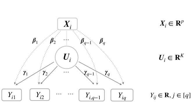
Figure 1: A schematic diagram of the proposed model in (1). The subscript $i$ indicates the $i$th subject, out of $n$ independent subjects. The response variable $Y_{ij}$ can be discrete or continuous.

Our proposed covariate-adjusted generalized factor model in (1) is motivated by applications in testing fairness. In the context of educational assessment, the subject’s responses to questions are dependent on latent factors $\bm{U}_{i}$ such as students’ abilities and skills, and are potentially affected by observed covariates $\bm{X}_{i}^{c}$ such as age, gender, and race, among others (Linda M. Collins 2009). The intercept $\beta_{j0}$ is often interpreted as the difficulty level of item $j$ and referred to as the difficulty parameter in psychometrics (Hambleton & Swaminathan 2013, Reckase 2009). The capability of item $j$ to further differentiate individuals based on their latent abilities is captured by $\bm{\gamma}_{j}=(\gamma_{j1},\ldots,\gamma_{jK})^{\intercal}$, which are also referred to as discrimination parameters (Hambleton & Swaminathan 2013, Reckase 2009). The effects of observed covariates $\bm{X}_{i}^{c}$ on subject’s response to the $j$th question $Y_{ij}$, conditioned on latent abilities $\bm{U}_{i}$, are captured by $\bm{\beta}_{jc}=(\beta_{j1},\ldots,\beta_{jp_{*}})^{\intercal}$, which are referred to as DIF effects in psychometrics (Holland & Wainer 2012). This setting gives rise to the fairness problem of validating whether the response probabilities to the measurements differ across different genders, races, or countries of origin while holding their abilities and skills at the same level.

Given the observed data from $n$ independent subjects, we are interested in studying the relationships between $\bm{Y}_{i}$ and $\bm{X}_{i}^{c}$ after adjusting for the latent factors $\bm{U}_{i}$ in (1). Specifically, our goal is to test the statistical hypothesis $H_{0}:\beta_{js}=0$ versus $H_{a}:\beta_{js}\neq 0$ for $s\in[p_{*}]$, where $\beta_{js}$ is the regression coefficient for the $s$th covariate and the $j$th response, after adjusting for the latent factor $\bm{U}_{i}$. In many applications, the latent factors and factor loadings also carry important scientific interpretations such as students’ abilities and test items’ characteristics. This motivates us to perform statistical inference on the parameters $\beta_{j0}$, $\bm{\gamma}_{j}$, and $\bm{U}_{i}$ as well.

Remark 1.

The proposed model setup (1) is general and flexible as various functions $p_{ij}$’s could be used to model diverse types of response data in wide-ranging applications. For instance, in educational assessments, logistic factor model (Reckase 2009) with

$$p_{ij}(y\mid w_{ij})=\exp(w_{ij}y)/\{1+\exp(w_{ij})\},\quad y\in\{0,1\}$$

and probit factor model (Birnbaum 1968) with

$$p_{ij}(y\mid w_{ij})=\{\Phi(w_{ij})\}^{y}\{1-\Phi(w_{ij})\}^{1-y},\quad y\in\{0,1\}$$

where $\Phi(\cdot)$ is the cumulative density function of standard normal distribution, are widely used to model the binary responses, indicating correct or incorrect answers to the test items. Such types of models are often referred to as item response theory models (Reckase 2009). In economics and finances, linear factor models with $p_{ij}(y\mid w_{ij})\propto\exp\{-(y-w_{ij})^{2}/(2\sigma^{2})\}$, where $y\in\mathbb{R}$ and $\sigma^{2}$ is the variance parameter, are commonly used to model continuous responses, such as GDP, interest rate, and consumer index (Bai 2003, Bai & Li 2012, Stock & Watson 2016). Moreover, depending on the the observed responses, different types of function $p_{ij}$’s can be used to model the response from each item $j\in[q]$. Therefore, mixed types of data, which are common in educational measurements (Rijmen et al. 2003) and macroeconomic applications (Wang 2022), can also be analyzed by our proposed model.

Remark 2.

In addition to testing fairness, the considered model finds wide-ranging applications in the real world. For instance, in genomics, the gene expression status may depend on unmeasured confounders or latent biological factors and also be associated with the variables of interest including medical treatment, disease status, and gender (Wang et al. 2017, Du et al. 2023). The covariate-adjusted general factor model helps to investigate the effects of the variables of interest on gene expressions, controlling for the latent factors (Du et al. 2023). This setting is also applicable to other scenarios, such as brain imaging, where the activity of a brain region may depend on measurable spatial distance from neighboring regions and latent structures due to unmodeled factors (Leek & Storey 2008).

To analyze large-scale measurement data, we aim to develop a computationally efficient estimation method and to provide inference theory for quantifying uncertainty in the estimation. Motivated by recent work in high-dimensional factor analysis, we treat the latent factors as fixed parameters and apply a joint maximum likelihood method for estimation (Bai 2003, Fan et al. 2013, Chen et al. 2020). Specifically, we let the collection of the item responses from $n$ independent subjects be $\mathbf{Y}=(\bm{Y}_{1},\dots,\bm{Y}_{n})_{n\times q}^{\intercal}$ and the design matrix of observed covariates to be $\mathbf{X}=(\bm{X}_{1},\dots,\bm{X}_{n})_{n\times p}^{\intercal}$. For model parameters, the discrimination parameters for all $q$ items are denoted as $\bm{\Gamma}=(\bm{\gamma}_{1},\dots,\bm{\gamma}_{q})_{q\times K}^{\intercal}$, while the intercepts and the covariate effects for all $q$ items are denoted as $\mathbf{B}=(\bm{\beta}_{1},\dots,\bm{\beta}_{q})_{q\times p}^{\intercal}$. The latent factors from all $n$ subjects are $\mathbf{U}=(\bm{U}_{1},\dots,\bm{U}_{n})_{n\times K}^{\intercal}$. Then, the joint log-likelihood function can be written as follows:

$$L(\mathbf{Y}\mid\bm{\Gamma},\mathbf{U},\mathbf{B},\mathbf{X})=\frac{1}{nq}\sum_{i=1}^{n}\sum_{j=1}^{q}l_{ij}(\beta_{j0}+\bm{\gamma}_{j}^{\intercal}\bm{U}_{i}+\bm{\beta}_{jc}^{\intercal}\bm{X}_{i}^{c}),$$ (2)

where the function $l_{ij}(w_{ij})=\log p_{ij}(Y_{ij}|w_{ij})$ is the individual log-likelihood function with $w_{ij}=\beta_{j0}+\bm{\gamma}_{j}^{\intercal}\bm{U}_{i}+\bm{\beta}_{jc}^{\intercal}\bm{X}_{i}^{c}$. We aim to obtain $(\widehat{\bm{\Gamma}},\widehat{\mathbf{U}},\widehat{\mathbf{B}})$ from maximizing the joint likelihood function $L(\mathbf{Y}\mid\bm{\Gamma},\mathbf{U},\mathbf{B},\mathbf{X})$.

While the estimators can be computed efficiently by maximizing the joint likelihood function through an alternating maximization algorithm (Collins et al. 2002, Chen et al. 2019), challenges emerge for performing statistical inference on the model parameters.

• One challenge concerns the model identifiability. Without additional constraints, the covariate effects are not identifiable due to the incorporation of covariates and their potential dependence on latent factors. The latent factors and factor loadings encounter similar identifiability issues as in traditional factor analysis (Bai & Li 2012, Fan et al. 2013). Ensuring that the model is statistically identifiable is the fundamental prerequisite for achieving model reliability and making valid inferences (Allman et al. 2009, Gu & Xu 2020).

• Another challenge arises from the nonlinearity of our proposed model. In the existing literature, most studies focus on the statistical inference for our proposed setting in the context of linear models (Bai & Li 2012, Fan et al. 2013, Wang et al. 2017). On the other hand, settings with general log-likelihood function $l_{ij}(w_{ij})$, including covariate-adjusted logistic and probit factor models, are less investigated. Common techniques for linear models are not applicable to the considered general nonlinear model setting.

Motivated by these challenges, we propose interpretable and practical identifiability conditions in Section 3.1. We then incorporate these conditions into the joint-likelihood-based estimation method in Section 3.2. Furthermore, we introduce a novel inference framework for performing statistical inference on $\bm{\beta}_{j}$, $\bm{\gamma}_{j}$, and $\bm{U}_{i}$ in Section 4.

3 Method

3.1 Model Identifiability

Identifiability issues commonly occur in latent variable models (Allman et al. 2009, Bai & Li 2012, Xu 2017). The proposed model in (1) has two major identifiability issues. The first issue is that the proposed model remains unchanged after certain linear transformations of both $\mathbf{B}$ and $\mathbf{U}$, causing the covariate effects together with the intercepts, represented by $\mathbf{B}$, and the latent factors, denoted by $\mathbf{U}$, to be unidentifiable. The second issue is that the model is invariant after an invertible transformation of both $\mathbf{U}$ and $\bm{\Gamma}$ as in the linear factor models (Bai & Li 2012, Fan et al. 2013), causing the latent factors $\mathbf{U}$ and factor loadings $\bm{\Gamma}$ to be undetermined.

Specifically, under the model setup in (1), we define the joint probability distribution of responses to be $P(\mathbf{Y}\mid\bm{\Gamma},\mathbf{U},\mathbf{B},\mathbf{X})=\prod_{i=1}^{n}\prod_{j=1}^{q}p_{ij}(Y_{ij}|w_{ij})$. The model parameters are identifiable if and only if for any response $\mathbf{Y}$, there does not exist $(\bm{\Gamma},\mathbf{U},\mathbf{B})\neq(\widetilde{\bm{\Gamma}},\widetilde{\mathbf{U}},\widetilde{\mathbf{B}})$ such that $P(\mathbf{Y}\mid\bm{\Gamma},\mathbf{U},\mathbf{B},\mathbf{X})=P(\mathbf{Y}\mid\widetilde{\bm{\Gamma}},\widetilde{\mathbf{U}},\widetilde{\mathbf{B}},\mathbf{X})$. The first issue concerning the identifiability of $\mathbf{B}$ and $\mathbf{U}$ is that for any $(\bm{\Gamma},\mathbf{U},\mathbf{B})$ and any transformation matrix $\mathbf{A}$, there exist $\widetilde{\bm{\Gamma}}=\bm{\Gamma}$, $\widetilde{\mathbf{U}}=\mathbf{U}+\mathbf{X}\mathbf{A}^{{\intercal}}$, and $\widetilde{\mathbf{B}}=\mathbf{B}-\bm{\Gamma}\mathbf{A}$ such that $P(\mathbf{Y}\mid\bm{\Gamma},\mathbf{U},\mathbf{B},\mathbf{X})=P(\mathbf{Y}\mid\widetilde{\bm{\Gamma}},\widetilde{\mathbf{U}},\widetilde{\mathbf{B}},\mathbf{X})$. This identifiability issue leads to the indeterminacy of the covariate effects and latent factors. The second issue is related to the identifiability of $\mathbf{U}$ and $\bm{\Gamma}$. For any $(\widetilde{\bm{\Gamma}},\widetilde{\mathbf{U}},\widetilde{\mathbf{B}})$ and any invertible matrix $\mathbf{G}$, there exist $\bar{\bm{\Gamma}}=\widetilde{\bm{\Gamma}}(\mathbf{G}^{{\intercal}})^{-1}$, $\bar{\mathbf{U}}=\widetilde{\mathbf{U}}\mathbf{G}$, and $\bar{\mathbf{B}}=\widetilde{\mathbf{B}}$ such that $P(\mathbf{Y}\mid\widetilde{\bm{\Gamma}},\widetilde{\mathbf{U}},\widetilde{\mathbf{B}},\mathbf{X})=P(\mathbf{Y}\mid\bar{\bm{\Gamma}},\bar{\mathbf{U}},\bar{\mathbf{B}},\mathbf{X})$. This causes the latent factors and factor loadings to be unidentifiable.

Remark 3.

Intuitively, the unidentifiable $\widetilde{\mathbf{B}}=\mathbf{B}-\bm{\Gamma}\mathbf{A}$ can be interpreted to include both direct and indirect effects of $\mathbf{X}$ on response $\mathbf{Y}$. We take the intercept and covariate effect on the first item $(\widetilde{\bm{\beta}}_{1})$ as an example and illustrate it in Figure 2. One part of $\widetilde{\bm{\beta}}_{1}$ is the direct effect from $\mathbf{X}$ onto $\mathbf{Y}$ (see the orange line in the left panel), whereas another part of $\widetilde{\bm{\beta}}_{1}$ may be explained through the latent factors $\mathbf{U}$, as the latent factors are unobserved and there are potential correlations between latent factors and observed covariates. The latter part of $\widetilde{\bm{\beta}}_{1}$ can be considered as the indirect effect (see the blue line in the right panel).

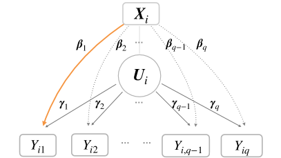
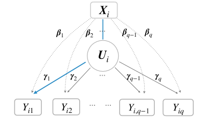
Figure 2: The direct effects (orange solid line in the left panel) and the indirect effects (blue solid line in the right panel) for item 1.

The first identifiability issue is a new challenge introduced by the covariate adjustment in the model, whereas the second issue is common in traditional factor models (Bai & Li 2012, Fan et al. 2013). Considering the two issues together, for any $(\bm{\Gamma},\mathbf{U},\mathbf{B})$, $\mathbf{A}$, and $\mathbf{G}$, there exist transformations $\widetilde{\bm{\Gamma}}=\bm{\Gamma}(\mathbf{G}^{{\intercal}})^{-1}$, $\widetilde{\mathbf{U}}=(\mathbf{U}+\mathbf{X}\mathbf{A}^{{\intercal}})\mathbf{G}$, and $\widetilde{\mathbf{B}}=\mathbf{B}-\bm{\Gamma}\mathbf{A}$ such that $P(\mathbf{Y}\mid\bm{\Gamma},\mathbf{U},\mathbf{B},\mathbf{X})=P(\mathbf{Y}\mid\widetilde{\bm{\Gamma}},\widetilde{\mathbf{U}},\widetilde{\mathbf{B}},\mathbf{X})$. In the rest of this subsection, we propose identifiability conditions to address these issues. For notation convenience, throughout the rest of the paper, we define $\bm{\phi}^{*}=(\bm{\Gamma}^{*},\mathbf{U}^{*},\mathbf{B}^{*})$ as the true parameters.

Identifiability Conditions

As described earlier, the correlation between the design matrix of covariates $\mathbf{X}$ and the latent factors $\mathbf{U}^{*}$ results in the identifiability issue of $\mathbf{B}^{*}$. In the psychometrics literature, the intercept $\beta_{j0}^{*}$ is commonly referred to as the difficulty parameter, while $\bm{\beta}_{jc}^{*}$ represents the effects of observed covariates, namely DIF effects, on the response to item $j$ (Reckase 2009, Holland & Wainer 2012). The different scientific interpretations motivate us to develop different identifiability conditions for $\beta_{j0}^{*}$ and $\bm{\beta}_{jc}^{*}$, respectively. Specifically, we propose a centering condition on $\mathbf{U}^{*}$ to ensure the identifiability of the intercept $\beta_{j0}^{*}$ for all items $j\in[q]$. On the other hand, to identify the covariate effects $\beta_{jc}^{*}$, a natural idea is to impose the covariate effects $\bm{\beta}_{jc}^{*}$ for all items $j\in[q]$ to be sparse, as shown in many regularized methods and item purification methods (Candell & Drasgow 1988, Fidalgo et al. 2000, Bauer et al. 2020, Belzak & Bauer 2020). In Chen et al. (2023a), an interpretable identifiability condition is proposed for selecting sparse covariate effects, yet this condition is specific to uni-dimensional covariates. Motivated by Chen et al. (2023a), we propose the following minimal $\ell_{1}$ condition applicable to general cases where the covariates are multi-dimensional. To better present the identifiability conditions, we write $\mathbf{A}=(\bm{a}_{0},\bm{a}_{1},\dots,\bm{a}_{p_{*}})\in\mathbb{R}^{K\times p}$ and define $\mathbf{A}_{c}=(\bm{a}_{1},\dots,\bm{a}_{p_{*}})\in\mathbb{R}^{K\times p_{*}}$ as the part applied to the covariate effects.

Condition 1.

(i) $\sum_{i=1}^{n}\bm{U}_{i}^{*}=\bm{0}_{K}$. (ii) $\sum_{j=1}^{q}\|\bm{\beta}_{jc}^{*}\|_{1}<\sum_{j=1}^{q}\|\bm{\beta}_{jc}^{*}-\mathbf{A}_{c}^{{\intercal}}\bm{\gamma}_{j}^{*}\|_{1}$ for any $\mathbf{A}_{c}\neq{\bm{0}}$.

Condition 1(i) assumes the latent abilities $\mathbf{U}^{*}$ are centered to ensure the identifiability of the intercepts $\bm{\beta}_{j0}^{*}$’s, which is commonly assumed in the item response theory literature (Reckase 2009). Condition 1(ii) is motivated by practical applications. For instance, in educational testing, practitioners need to identify and remove biased test items, correspondingly, items with non-zero covariate effects $(\beta_{js}^{*}\neq 0)$. In practice, most of the designed items are unbiased, and therefore, it is reasonable to assume that the majority of items have no covariate effects, that is, the covariate effects $\bm{\beta}_{jc}^{*}$’s are sparse (Holland & Wainer 2012, Chen et al. 2023a). Next, we present a sufficient and necessary condition for Condition 1(ii) to hold.

Proposition 1.

Condition 1(ii) holds if and only if for any $\bm{v}\in\mathbb{R}^{K}\setminus\{\bm{0}_{K}\}$,

$$\sum_{j=1}^{q}\big{|}\bm{v}^{\intercal}\bm{\gamma}_{j}^{*}\big{|}I{(\beta_{js}^{*}=0)}>\sum_{j=1}^{q}\mathop{\mathrm{sign}}(\beta_{js}^{*})\bm{v}^{\intercal}\bm{\gamma}_{j}^{*}I{(\beta_{js}^{*}\neq 0)},\quad\forall s\in[p_{*}].$$ (3)

Remark 4.

Proposition 1 implies that Condition 1(ii) holds when $\{j:\beta_{js}^{*}\neq 0\}$ is separated into $\{j:\beta_{js}^{*}>0\}$ and $\{j:\beta_{js}^{*}<0\}$ in a balanced way. With diversified signs of $\beta_{js}^{*}$, Proposition 1 holds when a considerable proportion of test items have no covariate effect $(\beta_{js}^{*}\neq 0)$. For example, when $\bm{\gamma}_{j}^{*}=m\bm{1}_{K}^{(k)}$ with $m>0$, Condition 1(ii) holds if and only if $\sum_{j=1}^{q}|m|\{-I(\beta_{js}^{*}/m>0)+I(\beta_{js}^{*}/m\leq 0)\}>0$ and $\sum_{j=1}^{q}|m|\{-I(\beta_{js}^{*}/m\geq 0)+I(\beta_{js}^{*}/m<0)\}<0$. With slightly more than $q/2$ items correspond to $\beta_{js}^{*}=0$, Condition 1(ii) holds. Moreover, if $\#\{j:\beta_{js}^{*}>0\}$ and $\#\{j:\beta_{js}^{*}<0\}$ are comparable, then Condition 1(ii) holds even when less than $q/2$ items correspond to $\beta_{js}^{*}=0$ and more than $q/2$ items correspond to $\beta_{js}^{*}\neq 0$. Though assuming a “sparse” structure, our assumption here differs from existing high-dimensional literature. In high-dimensional regression models, the covariate coefficient when regressing the dependent variable on high-dimensional covariates, is often assumed to be sparse, with the proportion of the non-zero covariate coefficients asymptotically approaching zero. In our setting, Condition 1(ii) allows for relatively dense settings where the proportion of items with non-zero covariate effects is some positive constant.

To perform simultaneous estimation and inference on $\bm{\Gamma}^{*}$ and $\mathbf{U}^{*}$, we consider the following identifiability conditions to address the second identifiability issue.

Condition 2.

(i) $(\mathbf{U}^{*})^{{\intercal}}\mathbf{U}^{*}$ is diagonal. (ii) $(\bm{\Gamma}^{*})^{\intercal}\bm{\Gamma}^{*}$ is diagonal. (iii) $n^{-1}(\mathbf{U}^{*})^{{\intercal}}\mathbf{U}^{*}=q^{-1}(\bm{\Gamma}^{*})^{\intercal}\bm{\Gamma}^{*}$.

Condition 2 is a set of widely used identifiability conditions in the factor analysis literature (Bai 2003, Bai & Li 2012, Wang 2022). For practical and theoretical benefits, we impose Condition 2 to address the identifiability issue related to $\mathbf{G}$. It is worth mentioning that this condition can be replaced by other identifiability conditions. For true parameters satisfying any identifiability condition, we can always find a transformation such that the transformed parameters satisfy our proposed Conditions 1–2 and the proposed estimation method and theoretical results in the subsequent sections still apply, up to such a transformation.

3.2 Joint Maximum Likelihood Estimation

In this section, we introduce a joint-likelihood-based estimation method for the covariate effects $\mathbf{B}$, the latent factors $\mathbf{U}$, and factor loadings $\bm{\Gamma}$ simultaneously. Incorporating Conditions 1–2 into the estimation procedure, we obtain the maximum joint-likelihood-based estimators for $\bm{\phi}^{*}=(\bm{\Gamma}^{*},\mathbf{U}^{*},\mathbf{B}^{*})$ that satisfy the proposed identifiability conditions.

With Condition 1, we address the identifiability issue related to the transformation matrix $\mathbf{A}$. Specifically, for any parameters $\bm{\phi}=(\bm{\Gamma},\mathbf{U},\mathbf{B})$, there exists a matrix $\mathbf{A}^{*}=(\bm{a}_{0}^{*},\mathbf{A}_{c}^{*})$ with $\mathbf{A}_{c}^{*}=\mathop{\mathrm{argmin}}_{\mathbf{A}_{c}\in\mathbb{R}^{K\times p_{*}}}\sum_{j=1}^{q}\|\bm{\beta}_{jc}-\mathbf{A}_{c}^{{\intercal}}\bm{\gamma}_{j}\|_{1}$ and $\bm{a}_{0}^{*}=-n^{-1}\sum_{i=1}^{n}(\bm{U}_{i}+\mathbf{A}_{c}^{*}\bm{X}_{i}^{c})$ such that the transformed matrices $\mathbf{U}^{*}=\mathbf{U}+\mathbf{X}(\mathbf{A}^{*})^{\intercal}$ and $\mathbf{B}^{*}=\mathbf{B}-\bm{\Gamma}\mathbf{A}^{*}$ satisfy Condition 1. The transformation idea naturally leads to the following estimation methodology for $\mathbf{B}^{*}$. To estimate $\mathbf{B}^{*}$ and $\mathbf{U}^{*}$ that satisfy Condition 1, we first obtain the maximum likelihood estimator $\widehat{\bm{\phi}}=(\widehat{\bm{\Gamma}},\widehat{\mathbf{U}},\widehat{\mathbf{B}})$ by

$$\widehat{\bm{\phi}}=\underset{\bm{\phi}\in\Omega_{\phi}}{\mathop{\mathrm{argmin}}}~{}-L(\mathbf{Y}\mid\bm{\phi},\mathbf{X}),$$ (4)

where the parameter space $\Omega_{\phi}$ is given as $\Omega_{\phi}=\{\bm{\phi}:\|\bm{\phi}\|_{\max}\leq C\}$ for some large $C$. To solve (4), we employ an alternating minimization algorithm. Specifically, for steps $t=0,1,\ldots$, we compute

$$\widehat{\bm{\Gamma}}^{(t+1)},\widehat{\mathbf{B}}^{(t+1)} =\mathop{\mathrm{argmin}}_{\begin{subarray}{c}\bm{\Gamma}\in\mathbb{R}^{q\times K},\;\mathbf{B}\in\mathbb{R}^{q\times p}\end{subarray}}-L(\mathbf{Y}\mid\bm{\Gamma},\mathbf{U}^{(t)},\mathbf{B},\mathbf{X});$$

$$\widehat{\mathbf{U}}^{(t+1)} =\mathop{\mathrm{argmin}}_{\mathbf{U}\in\mathbb{R}^{n\times K}}-L(\mathbf{Y}\mid\bm{\Gamma}^{(t+1)},\mathbf{U},\mathbf{B}^{(t+1)},\mathbf{X}),$$

until the quantity $\max\{\|\widehat{\bm{\Gamma}}^{(t+1)}-\widehat{\bm{\Gamma}}^{(t)}\|_{F},\|\widehat{\mathbf{U}}^{(t+1)}-\widehat{\mathbf{U}}^{(t)}\|_{F},\|\widehat{\mathbf{B}}^{(t+1)}-\widehat{\mathbf{B}}^{(t)}\|_{F}\}$ is less than some pre-specified tolerance value for convergence. We then estimate $\mathbf{A}_{c}$ by minimizing the $\ell_{1}$-norm

$$\widehat{\mathbf{A}}_{c}=\mathop{\mathrm{argmin}}_{\mathbf{A}_{c}\in\mathbb{R}^{K\times p_{*}}}\sum_{j=1}^{q}\|\widehat{\bm{\beta}}_{jc}-\mathbf{A}_{c}^{{\intercal}}\widehat{\bm{\gamma}}_{j}\|_{1}.$$ (5)

Next, we estimate $\widehat{\bm{a}}_{0}=-n^{-1}\sum_{i=1}^{n}(\widehat{\bm{U}}_{i}+\widehat{\mathbf{A}}_{c}\bm{X}_{i}^{c})$ and let $\widehat{\mathbf{A}}=(\widehat{\bm{a}}_{0},\widehat{\mathbf{A}}_{c})$. Given the estimators $\widehat{\mathbf{A}}$, $\widehat{\bm{\Gamma}}$, and $\widehat{\mathbf{B}},$ we then construct

$$\widehat{\mathbf{B}}^{*}=\widehat{\mathbf{B}}-\widehat{\bm{\Gamma}}\widehat{\mathbf{A}}~{}\mbox{ and }~{}\widetilde{\mathbf{U}}=\widehat{\mathbf{U}}+\mathbf{X}\widehat{\mathbf{A}}^{\intercal}$$

such that Condition 1 holds.

Recall that Condition 2 addresses the identifiability issue related to the invertible matrix $\mathbf{G}$. Specifically, for any parameters $(\bm{\Gamma},\mathbf{U})$, there exists a matrix $\mathbf{G}^{*}$ such that Condition 2 holds for $\mathbf{U}^{*}=(\mathbf{U}+\mathbf{X}(\mathbf{A}^{*})^{{\intercal}})\mathbf{G}^{*}$ and $\bm{\Gamma}^{*}=\bm{\Gamma}(\mathbf{G}^{*})^{-{\intercal}}$. Let $\mathcal{U}={\rm diag}(\varrho_{1},\dots,\varrho_{K})$ be a diagonal matrix that contains the $K$ eigenvalues of $(nq)^{-1}(\bm{\Gamma}^{{\intercal}}\bm{\Gamma})^{1/2}(\mathbf{U}+\mathbf{X}\mathbf{A}^{{\intercal}})^{{\intercal}}(\mathbf{U}+\mathbf{X}\mathbf{A}^{{\intercal}})$ $(\bm{\Gamma}^{{\intercal}}\bm{\Gamma})^{1/2}$ and let $\mathcal{V}$ be a matrix that contains its corresponding eigenvectors. We set $\mathbf{G}^{*}=(q^{-1}\bm{\Gamma}^{{\intercal}}\bm{\Gamma})^{1/2}$ $\mathcal{V}\mathcal{U}^{-1/4}$. To further estimate $\bm{\Gamma}^{*}$ and $\mathbf{U}^{*}$, we need to obtain an estimator for the invertible matrix $\mathbf{G}^{*}$. Given the maximum likelihood estimators obtained in (4) and $\widehat{\mathbf{A}}$ in (5), we estimate $\mathbf{G}^{*}$ via $\widehat{\mathbf{G}}=(q^{-1}\widehat{\bm{\Gamma}}^{{\intercal}}\widehat{\bm{\Gamma}})^{1/2}$ $\widehat{\mathcal{V}}\widehat{\mathcal{U}}^{-1/4}$ where $\widehat{\mathcal{U}}$ and $\widehat{\mathcal{V}}$ are matrices that contain the eigenvalues and eigenvectors of $(nq)^{-1}(\widehat{\bm{\Gamma}}^{{\intercal}}\widehat{\bm{\Gamma}})^{1/2}(\widehat{\mathbf{U}}+\mathbf{X}\widehat{\mathbf{A}}^{{\intercal}})^{{\intercal}}(\widehat{\mathbf{U}}+\mathbf{X}\widehat{\mathbf{A}}^{{\intercal}})$ $(\widehat{\bm{\Gamma}}^{{\intercal}}\widehat{\bm{\Gamma}})^{1/2}$, respectively. With $\widehat{\mathbf{G}}$ and $\widehat{\mathbf{A}}$, we now obtain the following transformed estimators that satisfy Condition 2:

$$\widehat{\bm{\Gamma}}^{*}=\widehat{\bm{\Gamma}}(\widehat{\mathbf{G}}^{{\intercal}})^{-1}~{}\mbox{ and }~{}\widehat{\mathbf{U}}^{*}=(\widehat{\mathbf{U}}+\mathbf{X}\widehat{\mathbf{A}}^{{\intercal}})\widehat{\mathbf{G}}.$$

To quantify the uncertainty of the proposed estimators, we will show that the proposed estimators are asymptotically normally distributed. Specifically, in Theorem 2 of Section 4, we establish the asymptotic normality result for $\widehat{\bm{\beta}}_{j}^{*}$, which allows us to make inference on the covariate effects $\bm{\beta}_{j}^{*}$. Moreover, as the latent factors $\bm{U}_{i}^{*}$ and factor loadings $\bm{\gamma}_{j}^{*}$ often have important interpretations in domain sciences, we are also interested in the inference on parameters $\bm{U}_{i}^{*}$ and $\bm{\gamma}_{j}^{*}$. In Theorem 2, we also derive the asymptotic distributions for estimators $\widehat{\bm{U}}_{i}^{*}$ and $\widehat{\bm{\gamma}}_{j}^{*}$, providing inference results for parameters $\bm{U}_{i}^{*}$ and $\bm{\gamma}_{j}^{*}$.

4 Theoretical Results

We propose a novel framework to establish the estimation consistency and asymptotic normality for the proposed joint-likelihood-based estimators $\widehat{\bm{\phi}}^{*}=(\widehat{\bm{\Gamma}}^{*},\widehat{\mathbf{U}}^{*},\widehat{\mathbf{B}}^{*})$ in Section 3. To establish the theoretical results for $\widehat{\bm{\phi}}^{*}$, we impose the following regularity assumptions.

Assumption 1.

There exist constants $M>0$, $\kappa>0$ such that:

(i) $\bm{\Sigma}_{u}^{*}=\lim_{n\rightarrow\infty}n^{-1}(\mathbf{U}^{*})^{{\intercal}}\mathbf{U}^{*}$ exists and is positive definite. For $i\in[n]$, $\|\bm{U}_{i}^{*}\|_{2}\leq M$.

(ii) $\bm{\Sigma}_{\gamma}^{*}=\lim_{q\rightarrow\infty}q^{-1}(\bm{\Gamma}^{*})^{{\intercal}}\bm{\Gamma}^{*}$ exists and is positive definite. For $j\in[q]$, $\|\bm{\gamma}_{j}^{*}\|_{2}\leq M$.

(iii) $\bm{\Sigma}_{x}=\lim_{n\rightarrow\infty}n^{-1}\sum_{i=1}^{n}\bm{X}_{i}\bm{X}_{i}^{{\intercal}}$ exists and $1/\kappa^{2}\leq\lambda_{\min}(\bm{\Sigma}_{x})\leq\lambda_{\max}(\bm{\Sigma}_{x})\leq\kappa^{2}$. For $i\in[n]$, $\max_{i}\|\bm{X}_{i}\|_{\infty}\leq M$.

(iv) $\bm{\Sigma}_{ux}^{*}=\lim_{n\rightarrow\infty}n^{-1}\sum_{i=1}^{n}\bm{U}_{i}^{*}\bm{X}_{i}^{{\intercal}}$ exists and $\|\bm{\Sigma}_{ux}^{*}\bm{\Sigma}_{x}^{-1}\|_{1,\infty}\leq M$. The eigenvalues of $(\bm{\Sigma}_{u}^{*}-\bm{\Sigma}_{ux}^{*}\bm{\Sigma}_{x}^{-1}(\bm{\Sigma}_{ux}^{*})^{{\intercal}})\bm{\Sigma}_{\gamma}^{*}$ are distinct.

Assumptions 1 is commonly used in the factor analysis literature. In particular, Assumptions 1(i)–(ii) correspond to Assumptions A-B in Bai (2003) under linear factor models, ensuring the compactness of the parameter space on $\mathbf{U}^{*}$ and $\bm{\Gamma}^{*}$. Under nonlinear factor models, such conditions on compact parameter space are also commonly assumed (Wang 2022, Chen et al. 2023b). Assumption 1(iii) is standard regularity conditions for the nonlinear setting that is needed to establish the concentration of the gradient and estimation error for the model parameters when $p$ diverges. In addition, Assumption 1(iv) is a crucial identification condition; similar conditions have been imposed in the existing literature such as Assumption G in Bai (2003) in the context of linear factor models and Assumption 6 in Wang (2022) in the context of nonlinear factor models without covariates.

Assumption 2.

For any $i\in[n]$ and $j\in[q]$, assume that $l_{ij}(\cdot)$ is three times differentiable, and we denote the first, second, and third order derivatives of $l_{ij}(w_{ij})$ with respect to $w_{ij}$ as $l_{ij}^{\prime}(w_{ij}),l_{ij}^{\prime\prime}(w_{ij})$, and $l_{ij}^{\prime\prime\prime}(w_{ij})$, respectively. There exist $M>0$ and $\xi\geq 4$ such that $\mathbb{E}(|l_{ij}^{\prime}(w_{ij})|^{\xi})\leq M$ and $|l_{ij}^{\prime}(w_{ij})|$ is sub-exponential with $\|l_{ij}^{\prime}(w_{ij})\|_{\varphi_{1}}\leq M$. Furthermore, we assume $\mathbb{E}\{l_{ij}^{\prime}(w_{ij}^{*})\}=0$. Within a compact space of $w_{ij}$, we have $b_{L}\leq-l_{ij}^{\prime\prime}(w_{ij})\leq b_{U}$ and $|l_{ij}^{\prime\prime\prime}(w_{ij})|\leq b_{U}$ for $b_{U}>b_{L}>0$.

Assumption 2 assumes smoothness on the log-likelihood function $l_{ij}(w_{ij})$. In particular, it assumes sub-exponential distributions and finite fourth-moments of the first order derivatives $l^{\prime}_{ij}(w_{ij})$. For commonly used linear or nonlinear factor models, the assumption is not restrictive and can be satisfied with a large $\xi$. For instance, consider the logistic model with $l_{ij}^{\prime}(w_{ij})=Y_{ij}-\exp(w_{ij})/\{1+\exp(w_{ij})\}$, we have $|l_{ij}^{\prime}(w_{ij})|\leq 1$ and $\xi$ can be taken as $\infty$. The boundedness conditions for $l_{ij}^{\prime\prime}(w_{ij})$ and $l_{ij}^{\prime\prime\prime}(w_{ij})$ are necessary to guarantee the convexity of the joint likelihood function. In a special case of linear factor models, $l_{ij}^{\prime\prime}(w_{ij})$ is a constant and the boundedness conditions naturally hold. For popular nonlinear models such as logistic factor models, probit factor models, and Poisson factor models, the boundedness of $l_{ij}^{\prime\prime}(w_{ij})$ and $l_{ij}^{\prime\prime\prime}(w_{ij})$ can also be easily verified.

Assumption 3.

For $\xi$ specified in Assumption 2 and a sufficiently small $\epsilon>0$, we assume as $n,q,p\rightarrow\infty$,

$$\frac{p}{\sqrt{n\wedge(pq)}}(nq)^{\epsilon+3/\xi}\to 0.$$ (6)

Assumption 3 is needed to ensure that the derivative of the likelihood function equals zero at the maximum likelihood estimator with high probability, a key property in the theoretical analysis. In particular, we need the estimation errors of all model parameters to converge to 0 uniformly with high probability. Such uniform convergence results involve delicate analysis of the convexity of the objective function, for which technically we need Assumption 3. For most of the popularly used generalized factor models, $\xi$ can be taken as any large value as discussed above, thus $(nq)^{\epsilon+3/\xi}$ is of a smaller order of $\sqrt{n\wedge(pq)}$, given small $\epsilon$. Specifically, Assumption 3 implies $p=o(n^{1/2}\wedge q)$ up to a small order term, an asymptotic regime that is reasonable for many educational assessments.

Next, we impose additional assumptions crucial to establishing the theoretical properties of the proposed estimators. One challenge for theoretical analysis is to handle the dependence between the latent factors $\mathbf{U}^{*}$ and the design matrix $\mathbf{X}$. To address this challenge, we employ the following transformed $\mathbf{U}^{0}$ that are orthogonal with $\mathbf{X}$, which plays an important role in establishing the theoretical results (see Supplementary Materials for details). In particular, for $i\in[n]$, we let $\bm{U}_{i}^{0}=(\mathbf{G}^{\ddagger})^{{\intercal}}(\bm{U}_{i}^{*}-\mathbf{A}^{\ddagger}\bm{X}_{i})$. Here ${\mathbf{G}}^{\ddagger}=(q^{-1}(\bm{\Gamma}^{*})^{{\intercal}}\bm{\Gamma}^{*})^{1/2}$ $\mathcal{V}^{*}(\mathcal{U}^{*})^{-1/4}$ and $\mathbf{A}^{\ddagger}=(\mathbf{U}^{*})^{{\intercal}}\mathbf{X}(\mathbf{X}^{\intercal}\mathbf{X})^{-1}$, where $\mathcal{U}^{*}={\rm diag}(\varrho_{1}^{*},\dots,\varrho_{K}^{*})$ with diagonal elements being the $K$ eigenvalues of $(nq)^{-1}((\bm{\Gamma}^{*})^{{\intercal}}\bm{\Gamma}^{*})^{1/2}(\mathbf{U}^{*})^{{\intercal}}(\mathbf{I}_{n}-\mathbf{P}_{x})\mathbf{U}^{*}((\bm{\Gamma}^{*})^{{\intercal}}\bm{\Gamma}^{*})^{1/2}$ with $\mathbf{P}_{x}=\mathbf{X}(\mathbf{X}^{{\intercal}}\mathbf{X})^{-1}\mathbf{X}^{{\intercal}}$ and $\mathcal{V}^{*}$ containing the matrix of corresponding eigenvectors. Under this transformation for $\bm{U}_{i}^{0}$, we further define $\bm{\gamma}_{j}^{0}=(\mathbf{G}^{\ddagger})^{-1}\bm{\gamma}_{j}^{*}$ and $\bm{\beta}_{j}^{0}=\bm{\beta}_{j}^{*}+(\mathbf{A}^{\ddagger})^{{\intercal}}\bm{\gamma}_{j}^{*}$ for $j\in[q]$, and write $\bm{Z}_{i}^{0}=((\bm{U}_{i}^{0})^{{\intercal}}$ $\bm{X}_{i}^{{\intercal}})^{{\intercal}}$ and $w_{ij}^{0}=(\bm{\gamma}_{j}^{0})^{{\intercal}}\bm{U}_{i}^{0}+(\bm{\beta}_{j}^{0})^{{\intercal}}\bm{X}_{i}$. These transformed parameters $\bm{\gamma}_{j}^{0}$’s, $\bm{U}_{i}^{0}$’s, and $\bm{\beta}_{j}^{0}$’s give the same joint likelihood value as that of the true parameters $\bm{\gamma}_{j}^{*}$’s, $\bm{U}_{i}^{*}$’s and $\bm{\beta}_{j}^{*}$’s, which facilitate our theoretical understanding of the joint-likelihood-based estimators.

Assumption 4.

(i) For any $j\in[q]$, $-n^{-1}\sum_{i=1}^{n}l_{ij}^{\prime\prime}(w_{ij}^{0})\bm{Z}_{i}^{0}(\bm{Z}_{i}^{0})^{{\intercal}}\overset{p}{\rightarrow}\bm{\Psi}_{jz}^{0}$ for some positive definite matrix $\bm{\Psi}_{jz}^{0}$ and $n^{-1/2}\sum_{i=1}^{n}l_{ij}^{\prime}(w_{ij}^{0})\bm{Z}_{i}^{0}\overset{d}{\rightarrow}\mathcal{N}(\bm{0},\bm{\Omega}_{jz}^{0})$.

(ii) For any $i\in[n]$, $-q^{-1}\sum_{j=1}^{q}l_{ij}^{\prime\prime}(w_{ij}^{0})\bm{\gamma}_{j}^{0}(\bm{\gamma}_{j}^{0})^{\intercal}\overset{p}{\rightarrow}\bm{\Psi}_{i\gamma}^{0}$ for some positive definite matrix $\bm{\Psi}_{i\gamma}^{0}$ and $q^{-1/2}\sum_{j=1}^{q}l_{ij}^{\prime}(w_{ij}^{0})\bm{\gamma}_{j}^{0}\overset{d}{\rightarrow}\mathcal{N}(\bm{0},\bm{\Omega}_{i\gamma}^{0})$.

Assumption 4 is a generalization of Assumption F(3)-(4) in Bai (2003) for linear models to the nonlinear setting. Specifically, we need Assumption 4(i) to derive the asymptotic distributions of the estimators $\widehat{\bm{\beta}}_{j}^{*}$ and $\widehat{\bm{\gamma}}_{j}^{*}$, and Assumption 4(ii) is used for establishing the asymptotic distribution of $\widehat{\bm{U}}_{i}^{*}$. Note that these assumptions are imposed on the log-likelihood derivative functions evaluated at the true parameters $w_{ij}^{0}$, $\bm{Z}_{i}^{0}$, and $\bm{\gamma}_{j}^{0}$. In general, for the popular generalized factor models, such assumptions hold with mild conditions. For example, under linear models, $l_{ij}^{\prime}(w_{ij})$ is the random error and $l_{ij}^{\prime\prime}(w_{ij})$ is a constant. Then $\bm{\Psi}_{jz}^{0}$ and $\bm{\Psi}_{i\gamma}^{0}$ naturally exist and are positive definite followed by Assumption 1. The limiting distributions of $n^{-1/2}\sum_{i=1}^{n}l_{ij}^{\prime}(w_{ij}^{0})\bm{Z}_{i}^{0}$ and $q^{-1/2}\sum_{j=1}^{q}l_{ij}^{\prime}(w_{ij}^{0})\bm{\gamma}_{j}^{0}$ can be derived by the central limit theorem under standard regularity conditions. Under logistic and probit models, $l_{ij}^{\prime}(w_{ij})$ and $l_{ij}^{\prime\prime}(w_{ij})$ are both finite inside a compact parameters space and similar arguments can be applied to show the validity of Assumption 4.

We present the following assumption to establish the theoretical properties of the transformed matrix $\widehat{\mathbf{A}}$ as defined in (5). In particular, we define $\mathbf{A}^{0}=(\mathbf{G}^{\ddagger})^{\intercal}\mathbf{A}^{\ddagger}$ and write $\mathbf{A}^{0}=(\bm{a}_{0}^{0},\dots,\bm{a}_{p_{*}}^{0})^{{\intercal}}$. Note that the estimation problem of (5) is related to the median regression problem with measurement errors. To understand the properties of this estimator, following existing M-estimation literature (He & Shao 1996, 2000), we define $\psi_{js}^{0}(\bm{a})=\bm{\gamma}_{j}^{0}\mathop{\mathrm{sign}}\{\beta_{js}^{0}+(\bm{\gamma}_{j}^{0})^{\intercal}(\bm{a}-\bm{a}_{s}^{0})\}$ and $\chi_{s}(\bm{a})=\sum_{j=1}^{q}\psi_{js}^{0}(\bm{a})$ for $j\in[q]$ and $s\in[p_{*}]$. We further define a perturbed version of $\psi_{js}^{0}(\bm{a})$, denoted as $\psi_{js}(\bm{a},\bm{\delta}_{js})$, as follows:

$$\psi_{js}(\bm{a},\bm{\delta}_{js})=\Big{(}\bm{\gamma}_{j}^{0}+\big{[}\frac{\bm{\delta}_{js}}{\sqrt{n}}\big{]}_{[1:K]}\Big{)}\mathop{\mathrm{sign}}\Big{\{}\beta_{js}^{0}+\big{[}\frac{\bm{\delta}_{js}}{\sqrt{n}}\big{]}_{K+1}-(\bm{\gamma}_{j}^{0}+\big{[}\frac{\bm{\delta}_{js}}{\sqrt{n}}\big{]}_{[1:K]})^{\intercal}(\bm{a}-\bm{a}_{s}^{0})\Big{\}},\,s\in[p_{*}]$$

where the perturbation

$$\bm{\delta}_{js} =\begin{pmatrix}\mathbf{I}_{K}&\bm{0}\\ \bm{0}&({\bm{1}}_{s}^{(p)})^{\intercal}\end{pmatrix}\Big{(}-\sum_{i=1}^{n}l_{ij}^{\prime\prime}(w_{ij}^{0})\bm{Z}_{i}^{0}(\bm{Z}_{i}^{0})^{\intercal}\Big{)}^{-1}\Big{(}\sqrt{n}\sum_{i=1}^{n}l_{ij}^{\prime}(w_{ij}^{0})\bm{Z}_{i}^{0}\Big{)},$$

is asymptotically normally distributed by Assumption 4. We define $\widehat{\chi}_{s}(\bm{a})=\sum_{j=1}^{q}\mathbb{E}\psi_{js}(\bm{a},\bm{\delta}_{js})$.

Assumption 5.

For $\chi_{s}(\bm{a})$, we assume that there exists some constant $c>0$ such that $\min_{\bm{a}\neq{\bm{0}}}|q^{-1}\chi_{s}(\bm{a})|>c$ holds for all $s\in[p_{*}]$. Assume there exists $\bm{a}_{s0}$ for each $s\in[p_{*}]$ such that $\widehat{\chi}_{s}(\bm{a}_{s0})$ $=0$ with $p\sqrt{n}\|\bm{\alpha}_{s0}\|\to 0$. In a neighbourhood of $\bm{\alpha}_{s0}$, $\widehat{\chi}_{s}(\bm{a})$ has a nonsingular derivative such that $\{q^{-1}\nabla_{\bm{a}}\widehat{\chi}_{s}(\bm{\alpha}_{s0})\}^{-1}=O(1)$ and $q^{-1}|\nabla_{\bm{a}}\widehat{\chi}_{s}(\bm{a})-\nabla_{\bm{a}}\widehat{\chi}_{s}(\bm{\alpha}_{s0})|\leq k|\bm{a}-\bm{\alpha}_{s0}|$. We assume $\iota_{nq,p}:=\max\big{\{}\|\bm{\alpha}_{s0}\|,q^{-1}\sum_{j=1}^{q}\psi_{js}(\bm{a}_{s0},\bm{\delta}_{js})\big{\}}=o\big{(}(p\sqrt{n})^{-1}\big{)}$.

Assumption 5 is crucial in addressing the theoretical difficulties of establishing the consistent estimation for $\mathbf{A}^{0}$, a challenging problem related to median regression with weakly dependent measurement errors. In Assumption 5, we treat the minimizer of $|\sum_{j=1}^{q}\psi(\bm{a},\bm{\delta}_{js})|$ as an $M$-estimator and adopt the Bahadur representation results in He & Shao (1996) for the theoretical analysis. For an ideal case where $\bm{\delta}_{js}$ are independent and normally distributed with finite variances, which corresponds to the setting in median regression with measurement errors (He & Liang 2000), these assumptions can be easily verified. Assumption 5 discusses beyond such an ideal case and covers general settings. In addition to independent and Gaussian measurement errors, this condition also accommodates the case when $\bm{\delta}_{js}$ are asymptotically normal and weakly dependent with finite variances, as implied by Assumption 4 and the conditional independence of $Y_{ij}$.

We want to emphasize that Assumption 5 allows for both sparse and dense settings of the covariate effects. Consider an example of $K=p=1$ and $\gamma_{j}=1$ for $j\in[q]$. Suppose $\beta_{js}^{*}$ is zero for all $j\in[q_{1}]$ and nonzero otherwise. Then this condition is satisfied as long as $\#\{j:\beta_{js}^{*}>0\}$ and $\#\{j:\beta_{js}^{*}<0\}$ are comparable, even when the sparsity level $q_{1}$ is small.

Under the proposed assumptions, we next present our main theoretical results.

Theorem 1 (Average Consistency).

Suppose the true parameters $\bm{\phi}^{*}=(\bm{\Gamma}^{*},\mathbf{U}^{*},\mathbf{B}^{*})$ satisfy identifiability conditions 1–2. Under Assumptions 1–5, we have

$$q^{-1}\|\widehat{\mathbf{B}}^{*}-\mathbf{B}^{*}\|_{F}^{2} =O_{p}\left({\frac{p^{2}\log qp}{n}}+{\frac{p\log n}{q}}\right);$$ (7)

if we further assume $p^{3/2}(nq)^{\epsilon+3/\xi}(p^{1/2}n^{-1/2}+q^{-1/2})=o(1)$, then we have

$$n^{-1}\|\widehat{\mathbf{U}}^{*}-\mathbf{U}^{*}\|_{F}^{2} =O_{p}\left({\frac{p\log qp}{n}}+{\frac{\log n}{q}}\right);$$ (8)

$$q^{-1}\|\widehat{\bm{\Gamma}}^{*}-\bm{\Gamma}^{*}\|_{F}^{2} =O_{p}\left({\frac{p\log qp}{n}}+{\frac{\log n}{q}}\right).$$ (9)

Theorem 1 presents the average convergence rates of $\widehat{\bm{\phi}}^{*}$. Consider an oracle case with $\mathbf{U}^{*}$ and $\bm{\Gamma}^{*}$ known, the estimation of $\mathbf{B}^{*}$ reduces to an $M$-estimation problem. For $M$-estimators under general parametric models, it can be shown that the optimal convergence rates in squared $\ell_{2}$-norm is $O_{p}(p/n)$ under $p(\log p)^{3}/n\rightarrow 0$ (He & Shao 2000). In terms of our average convergence rate on $\widehat{\mathbf{B}}^{*}$, the first term in (7), $n^{-1}p^{2}\log(qp)$, approximately matches the convergence rate $O_{p}(p/n)$ up to a relatively small order term of $p\log(qp)$. The second term in (7), $q^{-1}p\log n$, is mainly due to the estimation error for the latent factor ${\mathbf{U}}^{*}$. In educational applications, it is common to assume the number of subjects $n$ is much larger than the number of items $q$. Under such a practical setting with $n\gg q$ and $p$ relatively small, the term $q^{-1}\log n$ in (8) dominates in the derived convergence rate of $\widehat{\mathbf{U}}^{*}$, which matches with the optimal convergence rate $O_{p}(q^{-1})$ for factor models without covariates (Bai & Li 2012, Wang 2022) up to a small order term.

Remark 5.

The additional condition $p^{3/2}(nq)^{\epsilon+3/\xi}(p^{1/2}n^{-1/2}+q^{-1/2})=o(1)$ in Theorem 1 is used to handle the challenges related to the invertible matrix $\mathbf{G}$ that affects the theoretical properties of $\widehat{\mathbf{U}}^{*}$ and $\widehat{\bm{\Gamma}}^{*}$. It is needed for establishing the estimation consistency of $\widehat{\mathbf{U}}^{*}$ and $\widehat{\bm{\Gamma}}^{*}$ but not for that of $\widehat{\mathbf{B}}^{*}$. With sufficiently large $\xi$ and small $\epsilon$, this assumption is approximately $p=o(n^{1/4}\wedge q^{1/3})$ up to a small order term.

Remark 6.

One challenge in establishing the estimation consistency for $\widehat{\bm{\phi}}^{*}$ arises from the unrestricted dependence structure between $\mathbf{U}^{*}$ and $\mathbf{X}$. If we consider the ideal case where the columns of $\mathbf{U}^{*}$ and $\mathbf{X}$ are orthogonal, i.e., $(\mathbf{U}^{*})^{{\intercal}}\mathbf{X}=\bm{0}_{K\times p}$, then we can achieve comparable or superior convergence rates with less stringent assumptions. Specifically, with Assumptions 1–3 only, we can obtain the same convergence rates for $\widehat{\mathbf{U}}^{*}$ and $\widehat{\bm{\Gamma}}^{*}$ as in (8) and (9), respectively. Moreover, with Assumptions 1–3, the average convergence rate for the consistent estimator of $\mathbf{B}^{*}$ is $O_{p}(n^{-1}p\log qp+q^{-1}\log n)$, which is tighter than (7) by a factor of $p$.

With estimation consistency results established, we next derive the asymptotic normal distributions for the estimators, which enable us to perform statistical inference on the true parameters.

Theorem 2 (Asymptotic Normality).

Suppose the true parameters $\bm{\phi}^{*}=(\bm{\Gamma}^{*},\mathbf{U}^{*},\mathbf{B}^{*})$ satisfy identifiability conditions 1–2. Under Assumptions 1–5, we have the asymptotic distributions as follows. Denote $\zeta_{nq,p}^{-2}=n^{-1}{p\log qp}+q^{-1}{\log n}$. If $p^{3/2}\sqrt{n}(nq)^{3/\xi}\zeta_{nq,p}^{-2}\to 0$, for any $j\in[q]$ and $\bm{a}\in\mathbb{R}^{p}$ with $\|\bm{a}\|_{2}=1$,

$$\sqrt{n}\bm{a}^{{\intercal}}(\bm{\Sigma}_{\beta,j}^{*})^{-1/2}(\widehat{\bm{\beta}}_{j}^{*}-\bm{\beta}_{j}^{*}) \overset{d}{\to}\mathcal{N}(0,1),$$ (10)

where $\bm{\Sigma}_{\beta,j}^{*}=(-(\mathbf{A}^{0})^{{\intercal}},\;\mathbf{I}_{p})(\bm{\Psi}_{jz}^{0})^{-1}\bm{\Omega}_{jz}^{0}(\bm{\Psi}_{jz}^{0})^{-1}(-(\mathbf{A}^{0})^{{\intercal}},\;\mathbf{I}_{p})^{{\intercal}}$, and for any $j\in[q]$,

$$\sqrt{n}(\bm{\Sigma}_{\gamma,j}^{*})^{-1/2}(\widehat{\bm{\gamma}}_{j}^{*}-\bm{\gamma}_{j}^{*}) \overset{d}{\to}\mathcal{N}({\bm{0}},\mathbf{I}_{K}),$$ (11)

where $\bm{\Sigma}_{\gamma,j}^{*}=\mathbf{G}^{\ddagger}(\mathbf{I}_{K},\;\bm{0})(\bm{\Psi}_{jz}^{0})^{-1}\bm{\Omega}_{jz}^{0}(\bm{\Psi}_{jz}^{0})^{-1}$ $(\mathbf{I}_{K},\;\bm{0})^{{\intercal}}(\mathbf{G}^{\ddagger})^{{\intercal}}$. Furthermore, for any $i\in[n]$, if $q=O(n)$ and $p^{3/2}\sqrt{q}(nq)^{3/\xi}\zeta_{nq,p}^{-2}\to 0$,

$$\sqrt{q}(\bm{\Sigma}_{u,i}^{*})^{-1/2}(\widehat{\bm{U}}_{i}^{*}-\bm{U}_{i}^{*}) \overset{d}{\to}\mathcal{N}({\bm{0}},\mathbf{I}_{K}),$$ (12)

where $\bm{\Sigma}_{u,i}^{*}=(\mathbf{G}^{\ddagger})^{-{\intercal}}(\bm{\Psi}_{i\gamma}^{0})^{-1}\bm{\Omega}_{i\gamma}^{0}(\bm{\Psi}_{i\gamma}^{0})^{-1}(\mathbf{G}^{\ddagger})^{-1}$.

The asymptotic covariance matrices in Theorem 2 can be consistently estimated. Due to the space limitations, we defer the construction of the consistent estimators $\widehat{\bm{\Sigma}}_{\beta,j}^{*}$, $\widehat{\bm{\Sigma}}_{\gamma,j}^{*}$, and $\widehat{\bm{\Sigma}}_{u,i}^{*}$ to Supplementary Materials. Theorem 2 provides the asymptotic distributions for all individual estimators. In particular, with the asymptotic distributions and the consistent estimators $\widehat{\bm{\Sigma}}_{\beta,j}^{*}$ for the asymptotic covariance matrices, we can perform hypothesis testing on $\beta_{js}^{*}$ for $j\in[q]$ and $s\in[p_{*}]$. We reject the null hypothesis $\beta_{js}^{*}=0$ at significance level $\alpha$ if $|\sqrt{n}(\widehat{\sigma}_{\beta,js}^{*})^{-1}\widehat{\beta}_{js}^{*}|>\Phi^{-1}(1-\alpha/2)$, where $(\widehat{\sigma}_{\beta,js}^{*})^{2}$ is the $(s+1)$-th diagonal entry in $\widehat{\bm{\Sigma}}_{\beta,j}^{*}$.

For the asymptotic normality of $\widehat{\bm{\beta}}_{j}^{*}$, the condition $p^{3/2}\sqrt{n}(nq)^{3/\xi}(n^{-1}p\log qp+q^{-1}\log n)\to 0$ together with Assumption 3 gives $p=o\{n^{1/5}\wedge({q^{2}}/n)^{1/3}\}$ up to a small order term, and further implies $n\ll q^{2}$, which is consistent with established conditions in the existing factor analysis literature (Bai & Li 2012, Wang 2022). For the asymptotic normality of $\widehat{\bm{U}}_{i}^{*}$, the additional condition that $q=O(n)$ is a reasonable assumption in educational applications where the number of items $q$ is much fewer than the number of subjects $n$. In this case, the scaling conditions imply $p=o\{q^{1/3}\wedge(n^{2}/q)^{1/5}\}$ up to a small order term. Similarly for the asymptotic normality of $\widehat{\bm{\gamma}}_{j}^{*}$, the proposed conditions give $p=o\{n^{1/5}\wedge(q^{2}/n)^{1/3}\}$ up to a small order term.

Remark 7.

Similar to the discussion in Remark 6, the challenges arising from the unrestricted dependence between $\mathbf{U}^{*}$ and $\mathbf{X}$ also affect the derivation of the asymptotic distributions for the proposed estimators. If we consider the ideal case with $(\mathbf{U}^{*})^{{\intercal}}\mathbf{X}=\bm{0}_{K\times p}$, we can establish the asymptotic normality for all individual estimators under Assumptions 1–4 only and weaker scaling conditions. Specifically, when $(\mathbf{U}^{*})^{{\intercal}}\mathbf{X}=\bm{0}_{K\times p}$, the scaling condition becomes $p\sqrt{n}(nq)^{3/\xi}(n^{-1}p\log qp+q^{-1}\log n)\to 0$ for deriving asymptotic normality of $\widehat{\bm{\beta}}_{j}^{*}$ and $\widehat{\bm{\gamma}}_{j}^{*}$, which is milder than that for (10) and (11).

5 Simulation Study

In this section, we study the finite-sample performance of the proposed joint-likelihood-based estimator. We focus on the logistic latent factor model in (1) with $p_{ij}(y\mid w_{ij})=\exp(w_{ij}y)/\{1+\exp(w_{ij})\}$, where $w_{ij}=(\bm{\gamma}_{j}^{*})^{{\intercal}}\bm{U}_{i}^{*}+(\bm{\beta}_{j}^{*})^{{\intercal}}\bm{X}_{i}$. The logistic latent factor model is commonly used in the context of educational assessment and is also referred to as the item response theory model (Mellenbergh 1994, Hambleton & Swaminathan 2013). We apply the proposed method to estimate $\mathbf{B}^{*}$ and perform statistical inference on testing the null hypothesis $\beta_{js}^{*}=0$.

We start with presenting the data generating process. We set the number of subjects $n=\{300,500,1000,1500,2000\}$, the number of items $q=\{100,300,500\}$, the covariate dimension $p=\{5,10,30\}$, and the factor dimension $K=2$, respectively. We jointly generate $\bm{X}_{i}^{c}$ and $\bm{U}_{i}^{*}$ from $\mathcal{N}(\bm{0},\bm{\Sigma})$ where $\bm{\Sigma}_{ij}=\tau^{|i-j|}$ with $\tau\in\{0,0.2,0.5,0.7\}$. In addition, we set the loading matrix $\bm{\Gamma}_{[,k]}^{*}=\bm{1}_{k}^{(K)}\otimes\bm{v}_{k}$, where $\otimes$ is the Kronecker product and $\bm{v}_{k}$ is a $(q/K)$-dimensional vector with each entry generated independently and identically from Unif$[0.5,1.5]$. For the covariate effects $\mathbf{B}^{*}$, we set the intercept terms to equal $\beta_{j0}^{*}=0$. For the remaining entries in $\mathbf{B}^{*}$, we consider the following two settings: (1) sparse setting: $\beta_{js}^{*}=\rho$ for $s=1,\dots,p$ and $j=5s-4,\dots,5s$ and other $\beta_{js}^{*}$ are set to zero; (2) dense setting: $\beta_{js}^{*}=\rho$ for $s=1,\dots,p$ and $j=R_{s}q/5+1,\dots,(R_{s}+1)q/5$ with $R_{s}=s-5\lfloor{s/5}\rfloor$, and other $\beta_{js}^{*}$ are set to zero. Here, the signal strength is set as $\rho\in\{0.3,0.5\}$. Intuitively, in the sparse setting, we set 5 items to be biased for each covariate whereas in the dense setting, 20$\%$ of items are biased items for each covariate.

For better empirical stability, after reaching convergence in the proposed alternating maximization algorithm and transforming the obtained MLEs into ones that satisfy Conditions 1–2, we repeat another round of maximization and transformation. We take the significance level at $5\%$ and calculate the averaged type I error based on all the entries $\beta_{js}^{*}=0$ and the averaged power for all non-zero entries, over 100 replications. The averaged hypothesis testing results are presented in Figures 3–6 for $p=5$ and $p=30$, across different settings. Additional numerical results for $p=10$ are presented in the Supplementary Materials.

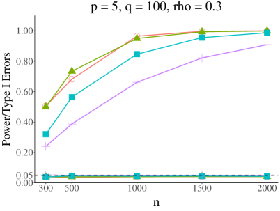
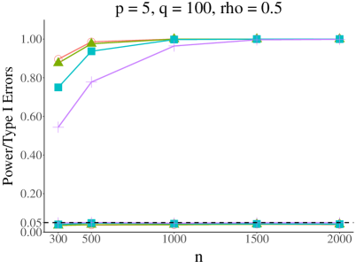
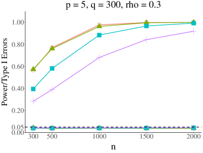
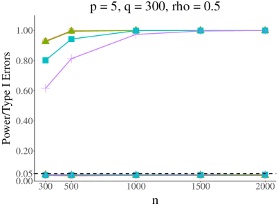
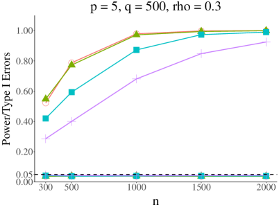
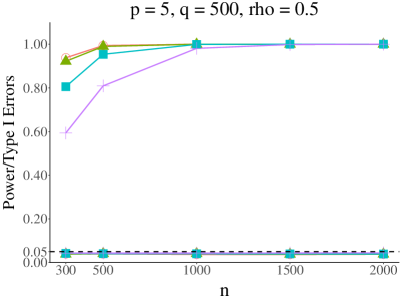
Figure 3: Powers and type I errors under sparse setting at $p=5$. Red Circles () denote correlation parameter $\tau=0$. Green triangles () represent the case $\tau=0.2$. Blue squares () indicate $\tau=0.5$. Purple crosses () represent the $\tau=0.7$.

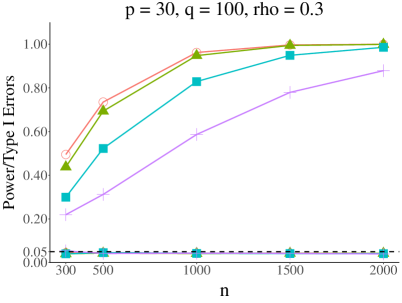
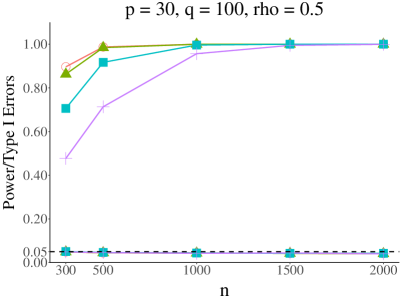
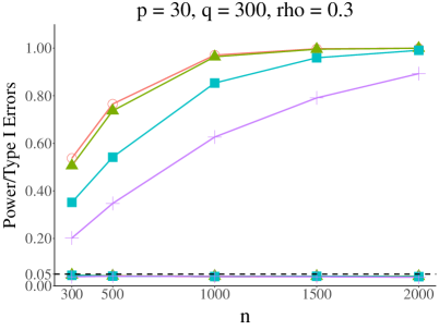
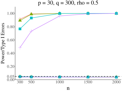
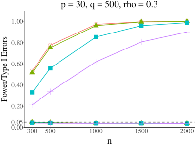
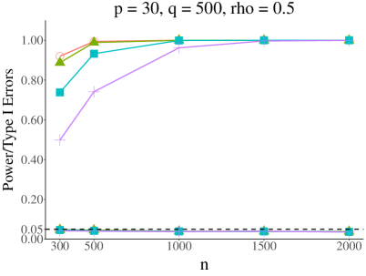
Figure 4: Powers and type I errors under sparse setting at $p=30$. Red Circles () denote correlation parameter $\tau=0$. Green triangles () represent the case $\tau=0.2$. Blue squares () indicate $\tau=0.5$. Purple crosses () represent the $\tau=0.7$.

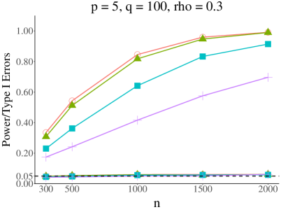
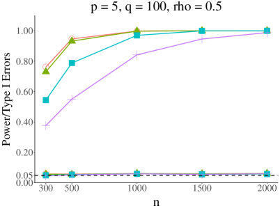
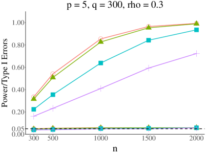
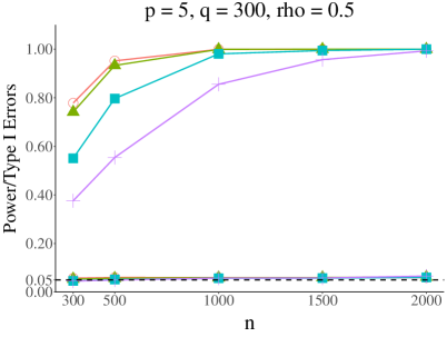
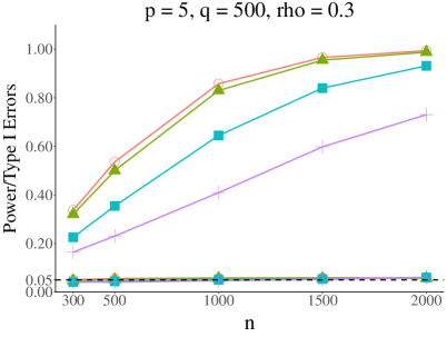
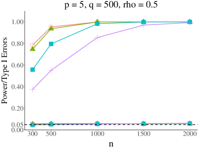
Figure 5: Powers and type I errors under dense setting at $p=5$. Red Circles () denote correlation parameter $\tau=0$. Green triangles () represent the case $\tau=0.2$. Blue squares () indicate $\tau=0.5$. Purple crosses () represent the $\tau=0.7$.

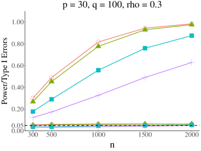
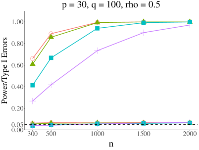
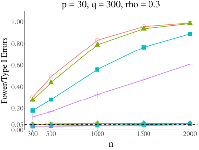
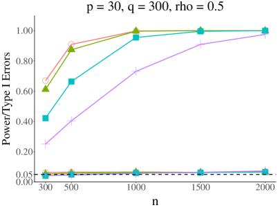
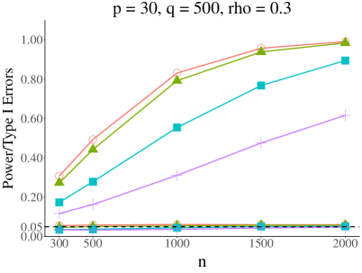
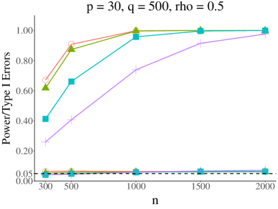
Figure 6: Powers and type I errors under dense setting at $p=30$. Red Circles () denote correlation parameter $\tau=0$. Green triangles () represent the case $\tau=0.2$. Blue squares () indicate $\tau=0.5$. Purple crosses () represent the $\tau=0.7$.

From Figures 3–6, we observe that the type I errors are well controlled at the significance level $5\%$, which is consistent with the asymptotic properties of $\widehat{\mathbf{B}}^{*}$ in Theorem 2. Moreover, the power increases to one as the sample size $n$ increases across all of the settings we consider. Comparing the left panel $(\rho=0.3)$ to the right panel $(\rho=0.5)$ in Figures 3–6, we see that the power increases as we increase the signal strength $\rho$. Comparing the plots in Figures 3–4 to the corresponding plots in Figures 5–6, we see that the powers under the sparse setting (Figures 3–4) are generally higher than that of the dense setting (Figures 5–6). Nonetheless, our proposed method is generally stable under both sparse and dense settings. In addition, we observe similar results when we increase the covariate dimension $p$ from $p=5$ (Figures 3 and 5) to $p=30$ (Figures 4 and 6). We refer the reader to the Supplementary Materials for additional numerical results for $p=10$. Moreover, we observe similar results when we increase the test length $q$ from $q=100$ (top row) to $q=500$ (bottom row) in Figures 3–6. In terms of the correlation between $\mathbf{X}$ and $\mathbf{U}^{*}$, we observe that while the power converges to one as we increase the sample size, the power decreases as the correlation $\tau$ increases.

6 Data Application

We apply our proposed method to analyze the Programme for International Student Assessment (PISA) 2018 data. PISA is a worldwide testing program that compares the academic performances of 15-year-old students across many countries (OECD 2019). More than 600,000 students from 79 countries/economies, representing a population of 31 million 15-year-olds, participated in this program. The PISA 2018 used the computer-based assessment mode and the assessment lasted two hours for each student, with test items mainly evaluating students’ proficiency in mathematics, reading, and science domains. A total of 930 minutes of test items were used and each student took different combinations of the test items. In addition to the assessment questions, background questionnaires were provided to collect students’ information.

In this study, we focus on PISA 2018 data from Taipei. The observed responses are binary, indicating whether students’ responses to the test items are correct, and we use the popular item response theory model with the logit link (i.e., logistic latent factor model; Reckase 2009). Due to the block design nature of the large-scale assessment, each student was only assigned to a subset of the test items, and for the Taipei data, $86\%$ response matrix is unobserved. Note that this missingness can be considered as conditionally independent of the responses given the students’ characteristics. Our proposed method and inference results naturally accommodate such missing data and can be directly applied. Specifically, to accommodate the incomplete responses, we can modify the joint log-likelihood function in (2) into $L^{obs}(\mathbf{Y}\mid\bm{\Gamma},\mathbf{U},\mathbf{B},\mathbf{X})=\sum_{i=1}^{n}\sum_{j\in\mathcal{Q}_{i}}l_{ij}(\bm{\gamma}_{j}^{\intercal}\bm{U}_{i}+\bm{\beta}_{j}^{\intercal}\bm{X}_{i})$, where $\mathcal{Q}_{i}$ defines the set of questions to which the responses from student $i$ are observed. In this study, we include gender and 8 variables for school strata as covariates $(p_{*}=9)$. These variables record whether the school is public, in an urban place, etc. After data preprocessing, we have $n=6063$ students and $q=194$ questions. Following the existing literature (Reckase 2009, Millsap 2012), we take $K=3$ to interpret the three latent abilities measured by the math, reading, and science questions.

We apply the proposed method to estimate the effects of gender and school strata variables on students’ responses. We obtain the estimators of the gender effect for each PISA question and construct the corresponding $95\%$ confidence intervals. The constructed $95\%$ confidence intervals for the gender coefficients are presented in Figure 7. There are 10 questions highlighted in red as their estimated gender effect is statistically significant after the Bonferroni correction. Among the reading items, there is only one significant item and the corresponding confidence interval is below zero, indicating that this question is biased towards female test-takers, conditioning on the students’ latent abilities. Most of the confidence intervals corresponding to the biased items in the math and science sections are above zero, indicating that these questions are biased towards male test-takers. In social science research, it is documented that female students typically score better than male students during reading tests, while male students often outperform female students during math and science tests (Quinn & Cooc 2015, Balart & Oosterveen 2019). Our results indicate that there may exist potential measurement biases resulting in such an observed gender gap in educational testing. Our proposed method offers a useful tool to identify such biased test items, thereby contributing to enhancing testing fairness by providing practitioners with valuable information for item calibration.

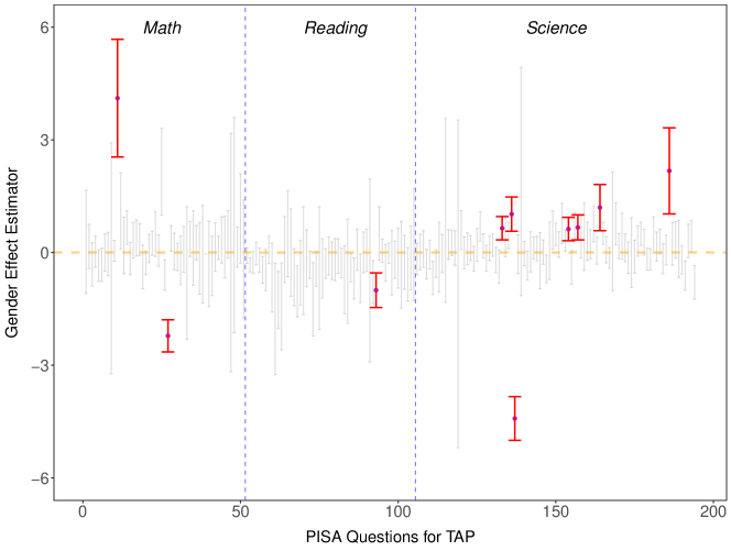
Figure 7: Confidence intervals for the effect of gender covariate on each PISA question using Taipei data. Red intervals correspond to confidence intervals for questions with significant gender bias after Bonferroni correction. (For illustration purposes, we omit the confidence intervals with the upper bounds exceeding 6 and the lower bounds below -6 in this figure).

Item code	Item Title	Female ($\%$)	Male ($\%$)	p-value
Mathematics
CM496Q01S	Cash Withdrawal	51.29	58.44	2.77$\times 10^{-7}\;(+)$
CM800Q01S	Computer Games	96.63	93.61	$<1\times 10^{-8}\;(-)$
Reading
CR466Q06S	Work Right	91.91	86.02	1.95$\times 10^{-5}\;(-)$
Science
CS608Q01S	Ammonoids	57.68	68.15	4.65$\times 10^{-5}\;(+)$
CS643Q01S	Comparing Light Bulbs	68.57	73.41	1.08$\times 10^{-5}\;(+)$
CS643Q02S	Comparing Light Bulbs2	63.00	57.50	4.64$\times 10^{-4}\;(-)$
CS657Q03S	Invasive Species	46.00	54.36	8.47$\times 10^{-5}\;(+)$
CS527Q04S	Extinction of Dinosours3	36.19	50.18	8.13$\times 10^{-5}\;(+)$
CS648Q02S	Habitable Zone	41.69	45.19	1.34$\times 10^{-4}\;(+)$
CS607Q01S	Birds and Caterpillars	88.14	91.47	1.99$\times 10^{-4}\;(+)$

Table 1: Proportion of full credit in females and males to significant items of PISA2018 in Taipei. $(+)$ and $(-)$ denote the items with positively and negatively estimated gender effects, respectively.

To further illustrate the estimation results, Table 1 lists the $p$-values for testing the gender effect for each of the identified 10 significant questions, along with the proportions of female and male test-takers who answered each question correctly. We can see that the signs of the estimated gender effect by our proposed method align with the disparities in the reported proportions between females and males. For example, the estimated gender effect corresponding to the item “CM496Q01S Cash Withdrawal” is positive with a $p$-value of $2.77\times 10^{-7}$, implying that this question is statistically significantly biased towards male test-takers. This is consistent with the observation that in Table 1, $58.44\%$ of male students correctly answered this question, which exceeds the proportion of females, $51.29\%$.

Besides gender effects, we estimate the effects of school strata on the students’ response and present the point and interval estimation results in the left panel of Figure 8. All the detected biased questions are from math and science sections, with 6 questions for significant effects of whether attending public school and 5 questions for whether residing in rural areas. To further investigate the importance of controlling for the latent ability factors, we compare results from our proposed method with the latent factors, to the results from directly regressing responses on covariates without latent factors. From the right panel of Figure 8, we can see that without conditioning on the latent factors, there are excessive items detected for the covariate of whether the school is public or private. On the other hand, there are no biased items detected if we only apply generalized linear regression to estimate the effect of the covariate of whether the school is in rural areas.

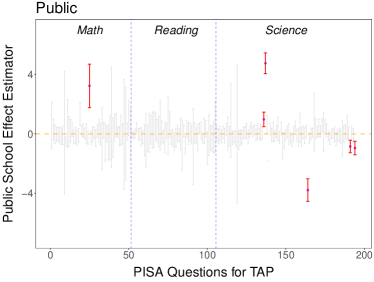
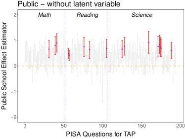
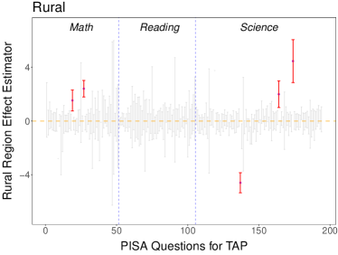
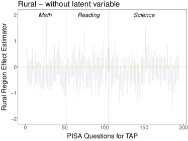
Figure 8: Confidence intervals for the effect of school stratum covariate on each PISA question. Red intervals correspond to confidence intervals for questions with significant school stratum bias after Bonferroni correction.

7 Discussion

In this work, we study the covariate-adjusted generalized factor model that has wide interdisciplinary applications such as educational assessments and psychological measurements. In particular, new identifiability issues arise due to the incorporation of covariates in the model setup. To address the issues and identify the model parameters, we propose novel and interpretable conditions, crucial for developing the estimation approach and inference results. With model identifiability guaranteed, we propose a computationally efficient joint-likelihood-based estimation method for model parameters. Theoretically, we obtain the estimation consistency and asymptotic normality for not only the covariate effects but also latent factors and factor loadings.

There are several future directions motivated by the proposed method. In this manuscript, we focus on the case in which $p$ grows at a slower rate than the number of subjects $n$ and the number of items $q$, a common setting in educational assessments. It is interesting to further develop estimation and inference results under the high-dimensional setting in which $p$ is larger than $n$ and $q$. Moreover, in this manuscript, we assume that the dimension of the latent factors $K$ is fixed and known. One possible generalization is to allow $K$ to grow with $n$ and $q$. Intuitively, an increasing latent dimension $K$ makes the identifiability and inference issues more challenging due to the increasing degree of freedom of the transformation matrix. With the theoretical results in this work, another interesting related problem is to further develop simultaneous inference on group-wise covariate coefficients, which we leave for future investigation.

References

- (1)
- Allman et al. (2009) Allman, E. S., Matias, C. & Rhodes, J. A. (2009), ‘Identifiability of parameters in latent structure models with many observed variables’, Annals of Statistics 37(6A), 3099–3132.
- Bai (2003) Bai, J. (2003), ‘Inferential theory for factor models of large dimensions’, Econometrica 71(1), 135–171.
- Bai & Li (2012) Bai, J. & Li, K. (2012), ‘Statistical analysis of factor models of high dimension’, Annals of Statistics 40(1), 436 – 465.
- Balart & Oosterveen (2019) Balart, P. & Oosterveen, M. (2019), ‘Females show more sustained performance during test-taking than males’, Nature Communications 10(1), 3798.
- Bauer et al. (2020) Bauer, D. J., Belzak, W. C. & Cole, V. T. (2020), ‘Simplifying the assessment of measurement invariance over multiple background variables: Using regularized moderated nonlinear factor analysis to detect differential item functioning’, Structural Equation Modeling: A Multidisciplinary Journal 27(1), 43–55.
- Bechger & Maris (2015) Bechger, T. M. & Maris, G. (2015), ‘A statistical test for differential item pair functioning’, Psychometrika 80(2), 317–340.
- Belzak & Bauer (2020) Belzak, W. & Bauer, D. J. (2020), ‘Improving the assessment of measurement invariance: Using regularization to select anchor items and identify differential item functioning.’, Psychological Methods 25(6), 673–690.
- Bing et al. (2024) Bing, X., Cheng, W., Feng, H. & Ning, Y. (2024), ‘Inference in high-dimensional multivariate response regression with hidden variables’, Journal of the American Statistical Association, in press .
- Birnbaum (1968) Birnbaum, A. (1968), Some latent trait models and their use in inferring an examinee’s ability, in F. M. Lord & M. R. Novick, eds, ‘Statistical Theories of Mental Test Scores’, Addison-Wesley, Reading, MA, pp. 395–479.
- Candell & Drasgow (1988) Candell, G. L. & Drasgow, F. (1988), ‘An iterative procedure for linking metrics and assessing item bias in item response theory’, Applied Psychological Measurement 12(3), 253–260.
- Carvalho et al. (2008) Carvalho, C. M., Chang, J., Lucas, J. E., Nevins, J. R., Wang, Q. & West, M. (2008), ‘High-dimensional sparse factor modeling: applications in gene expression genomics’, Journal of the American Statistical Association 103(484), 1438–1456.
- Chen et al. (2023a) Chen, Y., Li, C., Ouyang, J. & Xu, G. (2023a), ‘DIF statistical inference without knowing anchoring items’, Psychometrika 88(4), 1097–1122.
- Chen et al. (2023b) Chen, Y., Li, C., Ouyang, J. & Xu, G. (2023b), ‘Statistical inference for noisy incomplete binary matrix’, Journal of Machine Learning Research 24(95), 1–66.
- Chen et al. (2019) Chen, Y., Li, X. & Zhang, S. (2019), ‘Joint maximum likelihood estimation for high-dimensional exploratory item factor analysis’, Psychometrika 84, 124–146.
- Chen et al. (2020) Chen, Y., Li, X. & Zhang, S. (2020), ‘Structured latent factor analysis for large-scale data: Identifiability, estimability, and their implications’, Journal of the American Statistical Association 115(532), 1756–1770.
- Collins et al. (2002) Collins, M., Dasgupta, S. & Schapire, R. E. (2002), ‘A generalization of principal components analysis to the exponential family’, Advances in Neural Information Processing Systems pp. 617–624.
- Du et al. (2023) Du, J.-H., Wasserman, L. & Roeder, K. (2023), ‘Simultaneous inference for generalized linear models with unmeasured confounders’, arXiv preprint arXiv:2309.07261 .
- Fan et al. (2013) Fan, J., Liao, Y. & Mincheva, M. (2013), ‘Large covariance estimation by thresholding principal orthogonal complements’, Journal of the Royal Statistical Society Series B: Statistical Methodology 75(4), 603–680.
- Fidalgo et al. (2000) Fidalgo, A., Mellenbergh, G. J. & Muñiz, J. (2000), ‘Effects of amount of DIF, test length, and purification type on robustness and power of Mantel-Haenszel procedures’, Methods of Psychological Research Online 5(3), 43–53.
- Frichot et al. (2013) Frichot, E., Schoville, S. D., Bouchard, G. & François, O. (2013), ‘Testing for associations between loci and environmental gradients using latent factor mixed models’, Molecular Biology and Evolution 30(7), 1687–1699.
- Gerard & Stephens (2020) Gerard, D. & Stephens, M. (2020), ‘Empirical Bayes shrinkage and false discovery rate estimation, allowing for unwanted variation’, Biostatistics 21(1), 15–32.
- Gu & Xu (2020) Gu, Y. & Xu, G. (2020), ‘Partial identifiability of restricted latent class models’, Annals of Statistics 48(4), 2082–2107.
- Hambleton & Swaminathan (2013) Hambleton, R. K. & Swaminathan, H. (2013), Item response theory: Principles and applications, Springer Science & Business Media.
- He & Liang (2000) He, X. & Liang, H. (2000), ‘Quantile regression estimates for a class of linear and partially linear errors-in-variables models’, Statistica Sinica 10, 129–140.
- He & Shao (1996) He, X. & Shao, Q.-M. (1996), ‘A general Bahadur representation of M-estimators and its application to linear regression with nonstochastic designs’, Annals of Statistics 24(6), 2608 – 2630.
- He & Shao (2000) He, X. & Shao, Q.-M. (2000), ‘On parameters of increasing dimensions’, Journal of Multivariate Analysis 73(1), 120–135.
- Holland & Wainer (2012) Holland, P. W. & Wainer, H. (2012), Differential item functioning, Routledge.
- Kopf et al. (2015) Kopf, J., Zeileis, A. & Strobl, C. (2015), ‘A framework for anchor methods and an iterative forward approach for DIF detection’, Applied Psychological Measurement 39(2), 83–103.
- Lam et al. (2011) Lam, C., Yao, Q. & Bathia, N. (2011), ‘Estimation of latent factors for high-dimensional time series’, Biometrika 98(4), 901–918.
- Leek & Storey (2008) Leek, J. T. & Storey, J. D. (2008), ‘A general framework for multiple testing dependence’, Proceedings of the National Academy of Sciences 105(48), 18718–18723.
- Linda M. Collins (2009) Linda M. Collins, S. T. L. (2009), Latent Class and Latent Transition Analysis: With Applications in the Social, Behavioral, and Health Sciences, John Wiley & Sons, New York.
- Mellenbergh (1994) Mellenbergh, G. J. (1994), ‘Generalized linear item response theory’, Psychological Bulletin 115(2), 300.
- Millsap (2012) Millsap, R. E. (2012), Statistical Approaches to Measurement Invariance, Routledge.
- OECD (2019) OECD (2019), PISA 2018 Assessment and Analytical Framework, PISA, OECD Publishing, Paris.
- Park et al. (2018) Park, Y. S., Xing, K. & Lee, Y.-S. (2018), ‘Explanatory cognitive diagnostic models: Incorporating latent and observed predictors’, Applied Psychological Measurement 42(5), 376–392.
- Quinn & Cooc (2015) Quinn, D. M. & Cooc, N. (2015), ‘Science achievement gaps by gender and race/ethnicity in elementary and middle school: Trends and predictors’, Educational Researcher 44(6), 336–346.
- Reboussin et al. (2008) Reboussin, B. A., Ip, E. H. & Wolfson, M. (2008), ‘Locally dependent latent class models with covariates: an application to under-age drinking in the USA’, Journal of the Royal Statistical Society: Series A (Statistics in Society) 171(4), 877–897.
- Reckase (2009) Reckase, M. (2009), Multidimensional Item Response Theory, Springer New York, NY.
- Rijmen et al. (2003) Rijmen, F., Tuerlinckx, F., De Boeck, P. & Kuppens, P. (2003), ‘A nonlinear mixed model framework for item response theory’, Psychological Methods 8(2), 185.
- Stock & Watson (2002) Stock, J. H. & Watson, M. W. (2002), ‘Forecasting using principal components from a large number of predictors’, Journal of the American Statistical Association 97(460), 1167–1179.
- Stock & Watson (2016) Stock, J. & Watson, M. (2016), Dynamic factor models, factor-augmented vector autoregressions, and structural vector autoregressions in macroeconomics, Vol. 2 of Handbook of Macroeconomics, Elsevier, pp. 415–525.
- Tay et al. (2016) Tay, L., Huang, Q. & Vermunt, J. K. (2016), ‘Item response theory with covariates (IRT-C) assessing item recovery and differential item functioning for the three-parameter logistic model’, Educational and Psychological Measurement 76(1), 22–42.
- Thissen (1988) Thissen, D. (1988), Use of item response theory in the study of group differences in trace lines, in H. E. Wainer & H. I. Braun, eds, ‘Test validity’, Lawrence Erlbaum Associates, Inc, Mahwah, NJ, pp. 147–172.
- Toch (1984) Toch, T. (1984), ‘Test organization, insurance firm settle bias suit’, Education Week .
- Tutz & Berger (2016) Tutz, G. & Berger, M. (2016), ‘Item-focussed trees for the identification of items in differential item functioning’, Psychometrika 81(3), 727–750.
- von Davier Matthias (2008) von Davier Matthias (2008), ‘A general diagnostic model applied to language testing data’, British Journal of Mathematical and Statistical Psychology 61(2), 287–307.
- Wang et al. (2023) Wang, C., Zhu, R. & Xu, G. (2023), ‘Using lasso and adaptive lasso to identify dif in multidimensional 2pl models’, Multivariate Behavioral Research 58(2), 387–407.
- Wang (2022) Wang, F. (2022), ‘Maximum likelihood estimation and inference for high dimensional generalized factor models with application to factor-augmented regressions’, Journal of Econometrics 229(1), 180–200.
- Wang et al. (2017) Wang, J., Zhao, Q., Hastie, T. & Owen, A. B. (2017), ‘Confounder adjustment in multiple hypothesis testing’, Annals of Statistics 45(5), 1863.
- Xu (2017) Xu, G. (2017), ‘Identifiability of restricted latent class models with binary responses’, Annals of Statistics 45(2), 675–707.