Finch: Sparse and Structured Array Programming with Control Flow

Abstract.

From FORTRAN to NumPy, arrays have revolutionized how we express computation. However, arrays in these, and almost all prominent systems, can only handle dense rectilinear integer grids. Real world arrays often contain underlying structure, such as sparsity, runs of repeated values, or symmetry. Support for structured data is fragmented and incomplete. Existing frameworks limit the array structures and program control flow they support to better simplify the problem.

In this work, we propose a new programming language, Finch, which supports both flexible control flow and diverse data structures. Finch facilitates a programming model which resolves the challenges of computing over structured arrays by combining control flow and data structures into a common representation where they can be co-optimized. Finch automatically specializes control flow to data so that performance engineers can focus on experimenting with many algorithms. Finch supports a familiar programming language of loops, statements, ifs, breaks, etc., over a wide variety of array structures, such as sparsity, run-length-encoding, symmetry, triangles, padding, or blocks. Finch reliably utilizes the key properties of structure, such as structural zeros, repeated values, or clustered non-zeros. We show that this leads to dramatic speedups in operations such as SpMV and SpGEMM, image processing, graph analytics, and a high-level tensor operator fusion interface.

1. Introduction

Arrays are the most fundamental abstraction in computer science. Arrays and lists are often the first-taught datastructure (Abelson and Sussman, 1996, Chapter 2.2), (Knuth, 1997, Chapter 2.2). Arrays are also universal across programming languages, from their introduction in Fortran in 1957 to present-day languages like Python (Backus et al., 1957), keeping more-or-less the same semantics. Modern array programming languages such as NumPy (Harris et al., 2020), SciPy (Virtanen et al., 2020), MatLab (Moler and Little, 2020), TensorFlow (Abadi et al., 2016), PyTorch (Paszke et al., 2019), and Halide (Ragan-Kelley et al., 2013) have pushed the limits of productive data processing with arrays, fueling breakthroughs in machine learning, scientific computing, image processing, and more.

The success and ubiquity of arrays is largely due to their simplicity. Since their introduction, multidimensional arrays have represented dense, rectilinear, integer grids of points. By dense, we mean that indices are mapped to value via a simple formula relating multidimensional space to linear memory. Consequently, dense arrays offer extensive compiler optimizations and many convenient interfaces. Compilers understand dense computations across many programming constructs, such as for and while loops, breaks, parallelism, caching, prefetching, multiple outputs, scatters, gathers, vectorization, loop-carry-dependencies, and more. A myriad of optimizations have been developed for dense arrays, such as loop fusion, loop tiling, loop unrolling, and loop interchange. However, while dense arrays are the easiest way to program for performance, the world is not all dense.

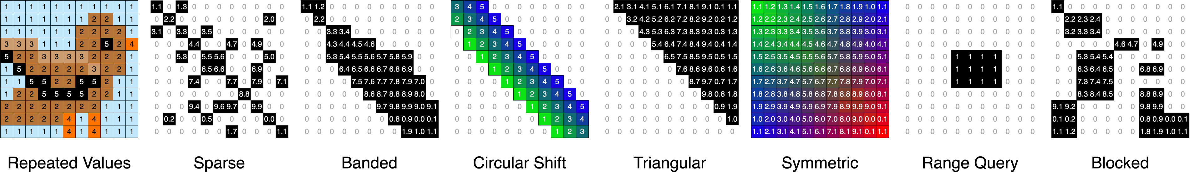
Figure 1. A few examples of matrix structures arising in practice

Our world is full of structured data.

Sparse arrays (which store only nonzero elements) describe networks, databases, and simulations (ABHYANKAR et al., [n. d.]; Bell and Koren, 2007; McAuley and Leskovec, 2013; Balay et al., 2020). Run-length encoding describes images and masks, geometry, and databases (such as a list of transactions with the date field all the same) (Shi, 2020; Golomb, 1966). Symmetry, bands, padding, and blocks arise due to modeling choices in scientific computing (e.g., higher order FEMs) as well as in intermediate structures in many linear solvers (e.g., GMRES) (Burns et al., 2020; Saad, 2003; O’Leary, 2009). In the context of machine learning, combinations of sparse and blocked matrices are increasingly under consideration (Dao et al., 2022). Even complex operators can be expressed as structured arrays. For example, a convolution with a filter can be expressed as a matrix multiplication with the Toeplitz matrix of all the circular shifts of the filter (Sze et al., 2017).

Currently, support for structured data is fragmented and incomplete. Experts must hand write variations of even the simplest kernels, like matrix multiply, for each data structure/data set and architecture to get performance. Implementations must choose a small set of features to support well, resulting in a compromise between program flexibility and data structure flexibility. Hand-written solutions are collected in diverse libraries like MKL, OpenCV, LAPACK or SciPy (Bradski et al., 2000; Anderson et al., 1999; Virtanen et al., 2020; Psarras et al., 2022). However, libraries will only ever support a subset of programs on a subset of data structure combinations. Even the most advanced libraries, such as the GraphBLAS, which support a wide variety of sparse operations over various semi-rings always lack support for other features, such as tensors, fused outputs, or runs of repeated values (Buluç et al., 2017; Mattson et al., 2019). While dense array compilers support an enormous variety of program constructs like early break and multiple left hand sides, they only support dense arrays (Ragan-Kelley et al., 2013; Grosser et al., 2012). Special-purpose compilers like TACO (Kjolstad et al., 2019), Taichi (Hu et al., 2019), StructTensor (Ghorbani et al., 2023), or CoRa (Fegade et al., 2022) which support a select subset of structured data structures (only sparse, or only ragged arrays) must compromise by greatly constraining the classes of programs which they support, such as tensor contractions. This trade-off is visualized in Tables LABEL:tab:features and LABEL:tab:data_structures.

Prior implementations are incomplete because the abstractions they use are tightly coupled with the specific data structures that they support. For example, TACO merge lattices represent Boolean logic over sets of non-zero values on an integer grid (Kjolstad et al., 2017). The polyhedral model allows various compilers to represent dense computations on affine regions (Grosser et al., 2012). Taichi enriches single static assignment form with a specialized instruction for accessing only a single sparse structure, but it supports more control flow  (Hu et al., 2019). These systems tightly couple their control flow to narrow classes of data structures to avoid the challenges that occur when we intersect complex control flow with structured data. There are two challenges:

Optimizations are specific to the indirection and patterns in data structures: These structures break the simple mapping between array elements and where they are stored in memory. For example, sparse arrays store lists of which coordinates are nonzero, whereas run-length-encoded arrays map several pixels to the same color value. These zero regions or repeated regions are optimization opportunities, and we must adapt the program to avoid repetitive work on these regions by referencing the stored structure.

Performance on structured data is highly algorithm dependent: The landscape of implementation decisions is dramatically unpredictable. For example, the asymptotic performance of sparse matrix multiplication can be impacted by the distribution of nonzeros, the sparse format, and the loop order (Ahrens et al., 2022; Zhang et al., 2021). This means that performance engineering for such kernels requires the exploration of a large design space, changing the algorithm as well as the data structures.

In this work, we propose a new programming language, Finch, which supports both flexible control flow and diverse data structures. Finch facilitates a programming model which resolves the challenges of computing over structured arrays by combining control flow and data structures into a common representation where they can be co-optimized. In particular, Finch automatically specializes the control flow to the data so that performance engineers can focus on experimenting with many algorithms. Finch supports a familiar programming language of loops, statements, if conditions, breaks, etc., over a wide variety of array structures, such as sparsity, run-length-encoding, symmetry, triangles, padding, or blocks. This support would be useless without the appropriate level of structural specialization; Finch reliably utilizes the key properties of structure, such as structural zeros, repeated values, or clustered non-zeros.

As an example, a programmer might explore different ways to intersect only the even integers of two lists (represented as sparse vectors with sorted indices). The control flow here is only useful if the first example differs from the next two in that it actually selects only even indices as the two integer lists are merged and different from the last in that it does not require another tensor:

⬇

for i = _

if i c[i]=a[i]*b[i]

end

end

⬇

for i = _

if i ap[i] = a[i]

end

end

for i = _

c[i] = ap[i] * b[i]

end

⬇

for i = _

cp[i] = a[i] * b[i]

end

for i = _

if i c[i] = cp[i]

end

end

⬇

for i = _

if i f[i] = 1

end

end

for i = _

c[i] = a[i] * b[i] * f[i]

end

1.1. Contributions

1. More complex array structures than ever before. We are the first to extend level-by-level hierarchical descriptions to capture banded, triangular, run-length-encoded, or sparse datasets, and any combination thereof. We have chosen a set of level formats that completely captures all combinations of relevant structural properties (zeros, repeated values, and/or blocks). Although many systems (TACO, Taichi, SPF, Ebb) (Chou et al., 2018; Hu et al., 2019; Strout et al., 2018; Bernstein et al., 2016) feature a flexible structure description, our level abstraction is more capable and extensible because it uses Looplets (Ahrens et al., 2023) to express the structure of each level.

2. A rich structured array programming language with for-loops and complex control flow constructs at the same level of productivity of dense arrays. To our knowledge, the Finch programming language is the first to support if-conditions, early breaks, and multiple left hand sides over structured data, as well as complex accesses such as affine indexing or scatter/gather of sparse or structured operands.

3. A compiler that specializes programs to data structures automatically, facilitating an expressive language that makes it easier to search the complex space of algorithms and data structures. Finch reliably utilizes four key properties of structure, such as structural zeros, repeated values, clustered non-zeros, and singletons.

4. Our compiler is highly extensible, evidenced by the variety of level formats and control flow constructs that we implement in this work. For example, Finch has been extended to support real-valued array indices with continuous arrays. Finch is also used as a compiler backend for the Python PyData/Sparse library (Abbasi, 2023).

5. We evaluate the efficiency, flexibility, and expressibility of our language in several case studies on a wide range of applications, demonstrating speedups over the state of the art in classic operations such as SpMV ($2.51\times$) and SpGEMM ($1.25\times$), to more complex applications such as graph analytics ($3.53\times$, reducing lines of code by $4\times$ over GraphBLAS), image processing ($19.5\times$), and the Python Array API ($28\times$).

This advances the state-of-the-art over the Looplets work (Ahrens et al., 2023). While Looplets presented a way to merge iterators over multiple single dimensional structures, we go further by combining single-dimensional looplets into multi-dimensional tensors and operating on them in a programming language with fully-featured control flow.

$\text{{lookup}}(seek,body)$: The Lookup looplet represents a randomly accessible region of an iterator. The body of the lookup is understood to have one less dimension than the lookup itself, as we have already “looked up” that index in the tensor by the time we reach the body. seek(i) is a function that updates state to the given index.
$\text{{run}}(body)$: The Run looplet represents a constant region of an iterator. The body of the run is understood to have one less dimension than the lookup itself, as all of the bodies are identical.
$\text{{phase}}(c:d,body)$: The Phase looplet represents a restriction of the range on which a loop should execute, and allows us to succinctly express the ranges on which children of compound looplets are defined.
$\text{{switch}}(cond,head,tail)$: The Switch looplet allows us to specialize the body of a looplet based on a condition, evaluated in the embedding context. If the condition is true, we use ‘head‘, otherwise we use ‘tail‘. Switch has a high lowering priority so we can see what’s inside of it and lower that appropriately. This also lifts the condition as high as possible into the loop nest. The condition is assumed to evaluate to a Boolean.
$\text{{thunk}}(preamble,body,epilogue)$: The Thunk looplet allows us to cache certain computations in the state under which the body will execute. This is useful for computing and caching the results of expensive computations.
$\text{{sequence}}(head,tail)$: The Sequence looplet represents the concatenation of two looplets. Both arguments must be phase looplets, and are assumed to be non-overlapping, covering, and in order.
$\text{{spike}}(body,tail)$: The Spike looplet represents a run followed by a single value. In this paper, Spike will be considered a shorthand for $\text{{sequence}}(\text{{phase}}(i:j-1,\text{{run}}(body)),\text{{phase}}(j:j,\text{{run}}(tail)))$. In the Finch compiler, spikes are handled with special care, since they are an opportunity to align the final run to the end of the root loop extent, without using any special bounds inference.
$\text{{stepper}}([seek],next,body)$: The stepper looplet represents a variable number of looplets, concatenated. Since our looplets may be skipped over due to conditions or various rewrites, the $seek$ function allows us to fast-forward the state to the start of the root loop extent when it comes time to lower the stepper. The $next$ function advances the state to the next iteration of the stepper.

Figure 2. The Looplet language, as understood in a correct execution of a Finch program.

2. Background

2.1. Looplets

Finch represents iteration patterns using Looplets, a language that decomposes datastructure iterators hierarchically. Looplets represent the control-flow structures needed to iterate over any given datastructure, or multiple datastructures simultaneously. In particular, Looplets are good at lifting code to the highest possible loop level and subdividing iteration hierarchically in coordinate space. Because Looplets are compiled with progressive lowering, structure-specific mathematical optimizations such as integrals, multiply by zero, etc. can be implemented using simple compiler passes like term rewriting and constant propagation during the intermediate lowering stages.

The Looplets are described in Figure 2. We simplify the presentation to focus on the semantics, rather than precise implementation. Several looplets introduce or modify variables in the scope of the target language. It is assumed that if a looplet introduces a variable, the child looplet will not modify that variable. For more background on Looplets, we recommend the original work (Ahrens et al., 2023).

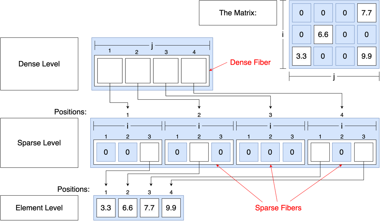
Figure 3. Levels in the fiber tree representation of a sparse matrix in CSC format, with a dense outer level and a sparse inner level. The element level holds the leaves of the tree.

2.2. Fiber Trees

Fiber-tree style tensor abstractions have been the subject of extensive study (Sze et al., 2017; Chou and Amarasinghe, 2022; Chou et al., 2018). The underlying idea is to represent a multi-dimensional tensor as a nested vector datastructure, where each level of the nesting corresponds to a dimension of the tensor. Thus, a matrix would be represented as a vector of vectors. This kind of abstraction lends itself to representing sparse tensors if we vary the type of vector used at each level in a tree. Thus, a sparse matrix might be represented as a dense vector of sparse vectors. The vector of subtensors in this abstraction is referred to as a fiber.

Instead of storing the data for each subfiber separately, most sparse tensor formats such as CSR, DCSR, and COO usually store the data for all fibers in a level contiguously. In this way, we can think of a level as a bulk allocator for fibers. Continuing the analogy, we can think of each fiber as being disambiguated by a position, or an index into the bulk pool of subfibers. The mapping $f$ from indices to subfibers is thus a mapping from an index and a position in a level to a subposition in a sublevel. Figure 3 shows a simple example of a level as a pool of fibers.

When we need to refer to a particular fiber at position $p$ in the level $l$, we may write $fiber(l,p)$. Note that the formation of fibers from levels is lazy, and the data underlying each fiber is managed entirely by the level, so the level may choose to overlap the storage between different fibers. Thus, the only unique data associated with $fiber(l,p)$ is the position $p$.

3. Bridging Looplets and Finch: The Tensor Interface

Arrays use multiple dimensions to organize data with respect to orthogonal concepts. Thus, the Finch language supports multi-dimensional arrays. Unfortunately, the Looplet abstraction is best suited towards iterators over a single dimension. Our level abstraction provides a bridge between the single dimensional iterators created from Looplets and the multi-dimensional fiber-tree abstractions common to tensor compilers. This bridge must address three challenges. First, while Looplets represent an instance of an iterator over a tensor, we may access the same tensor twice with different indices. Thus, the $unfurl$ function creates separate looplet nests for each iterator. Next, since Finch programs go beyond just single Einsums, they may read and write to the same data at different times. The $declare$, $freeze$, and $thaw$ functions provide machinery to manage transition between these states. Finally, we must be able to write looplet nests that modify tensors, as well as reading them. The $assemble$ function manages the allocation of new data in the tensor.

Additionally, prior fiber-tree representations focus on sparsity (where only the nonzero elements are represented) and treat sparse vectors as sets of represented points. Since our fiber-tree representation must handle other kinds of structure, such as diagonal, repeated, or constant values, we must generalize our fiber abstraction to allow arbitrary mappings from indices into a space of subfibers.

In the rest of this section, we discuss how these 5 core functions ($declare$, $freeze$, $thaw$, $unfurl$, and $assemble$) function as part of a life cycle abstraction that defines a level in Finch. These interfaces add to the level abstraction, expanding the types of data that they can express via mapping to Looplets and expanding the contexts in which they can be used. We then identify a taxonomy of four key structural properties exhibited in data. We implement several levels in this abstraction that capture all combinations of these structures, including specializations to zero dimensional tensors (scalars) and level structures that support different access patterns.

3.1. Tensor Lifecycle, Declare, Freeze, Thaw, Unfurl

Our simplified view of a level is enabled by our use of Looplets to represent the structure within each fiber. In fact, our level interface requires only 5 highly general operations, described below.

The first three of these functions, $declare$, $freeze$, and $thaw$, have to do with managing when tensors can be assumed mutable or immutable. As we use Looplets to represent iteration over a tensor, we must restrict the mutability of tensors while we iterate over them. For example, if a tensor declares it has a constant region from $i=2:5$, but some other part of the computation modifies the tensor at $i=3$, this would result in incorrect behavior. It is much easier to write correct Looplet code if we can assume that the tensor is immutable while we are reading from it. Thus, we introduce the notion that a tensor can be in read-only mode or update-only mode. In read-only mode, the tensor may only appear in the right-hand side of assignments . In update-only mode, the tensor may only appear in the left-hand side of an assignment, either being overwritten or incremented by some operator. We can switch between these modes using freeze and thaw functions. The $declare$ function is used to allocate a tensor, initialize it to some specified size and value, and leave it in update-only mode.

The $unfurl$ function is used to manage iteration over a subfiber. At the point when it comes time to iterate over a tensor, be in on the left or right hand side of an assignment, we call $unfurl$ to precompute whatever state and datastructures are necessary to return a looplet nest that would iterate over that level of a tensor. We call $unfurl$ directly before iterating over the corresponding loop, so it has access to any state variables introduced by freezing or thawing the tensor.

$declare(lvl,init,dims...)$: Declares the level to hold subtensors of size $dims$ and an initial value of $init$. Requires the level to be in read-only mode.

$freeze(lvl)$: Finalizes the updates in the level, and readies the level for reading. Requires the level to be in update-only mode.

$thaw(lvl)$: Prepares the level to accept updates. Requires the level to be in read-only mode.

$unfurl(fiber(lvl,pos),[ext],mode,[op],[rhs])$: When $ext$ is given, unfurls the fiber at position $pos$ in the level $lvl$ over the extent $ext$. When $mode=\text{{read}}$, returns a looplet nest over the values in the read-only fiber. When $mode=\text{{update}}$, returns a looplet nest over mutable subfibers in the update-only fiber. When applied to a scalar or leaf node, $ext$ is omitted and we may also use $op$ and $rhs$ to update the scalar value. Often, skipping over mutable locations allows the level to know which locations must be stored. Often, a dirty bit may be used in $tns$ to communicate whether the mutable subfiber has been written to, which allows the parent fiber to know whether the subfiber must be stored explicitly.

$assemble(lvl,pos_{start},pos_{stop})$: Allocates subfibers in the level from positions $pos_{start}$ to $pos_{stop}$. Usually, this function is only ever called on unassembled positions, but some levels (such as dense levels or bytemaps) may support reassembly.

Figure 4. The five functions that define a level.

Our view of a level as a fiber allocator implies an allocation function $assemble(tns,pos_{start}:pos_{stop})$, which allocates fibers at positions $pos_{start}:pos_{stop}$ in the level. We don’t specify a de-allocation function, instead relying on initialization to reset the fiber if it needs to be reused. While all of the previous functions are used to manage the lifecycle and iteration over a general tensor, $assemble$ is quite specific to the level abstraction, and the notion of positions within sublevels. Note: it was an intentional choice to hold the parent level responsible for managing the data of the sublevels, which positions they allocate, etc. This allows the parent level to reuse allocation logic from internal index datastructures. For example, a sparse level might use a list of indices to store which nonzeros are present, and when it comes time to resize that list, it could also call $assemble$ to resize the sublevel, reducing the number of branches in the code. The $assemble$ function lends itself particularly to a ”vector doubling” allocation approach, which we have found to be effective and flexible when managing the allocation of sparse left hand sides. This benefit is made clear in our case studies, where prior systems like TACO do not support all possible loop orderings and format combinations for sparse matrix multiply because they do not have a flexible enough allocation strategy, instead using a two-phase approach which requires computing a complicated closed-form kernel to iterate over the data twice to determine the number of required output nonzeros.

3.2. The 4 Key Structures

Sparse	Blocked	Runs	Singular	Corresponding Format
				Dense
			$\checkmark$	n/a
		$\checkmark$		DenseRLE
		$\checkmark$	$\checkmark$	n/a
	$\checkmark$			n/a
	$\checkmark$		$\checkmark$	n/a
	$\checkmark$	$\checkmark$		n/a
	$\checkmark$	$\checkmark$	$\checkmark$	n/a
$\checkmark$				Sparse
$\checkmark$			$\checkmark$	SparsePinpoint
$\checkmark$		$\checkmark$		SparseRLE
$\checkmark$		$\checkmark$	$\checkmark$	SparseInterval
$\checkmark$	$\checkmark$			SparseVBL
$\checkmark$	$\checkmark$		$\checkmark$	SparseBand
$\checkmark$	$\checkmark$	$\checkmark$		n/a
$\checkmark$	$\checkmark$	$\checkmark$	$\checkmark$	n/a

Figure 5. All combinations of our 4 structural properties and the corresponding formats we have chosen to represent them. Not all combinations are relevant. Note that blocks and runs need not be considered together because we must store a run length for each run, so there isn’t a significant storage benefit to combining them. Blocks and singletons only make sense in the context of sparsity.

In the Finch programming model, the programmer relies on the Finch compiler to specialize to the sequential properties of the data. In our experience, the main benefits of specializing to structure come from the following properties of the data:

• Sparsity Sparse data is data that is mostly zero, or some other fill value. When we specialize on this data, we can use annihilation ($x*0=0$), identity ($x*1=1$), or other constant propagation properties ($ifelse(false,x,y)=y$) to simplify the computation and avoid redundant work.

• Blocks Blocked data is a subset of sparse data where the nonzeros are clustered and occur adjacent to one another. This provides us with two opportunities: We can avoid storing the locations of the nonzeros individually, and we can use more efficient randomly accessible iterators within the block. (Im and Yelick, 2001; Vuduc et al., 2002; Ahrens et al., 2023).

• Runs Runs of repeated values may occur in dense or sparse code, cutting down on storage and allowing us to use integration rules such as

  for i = 1:n; s += x end} $\rightarrow$
          \mintinline

  julia

s += n * x or code motion to lift operations out of loops (Donenfeld et al., 2022; Ahrens et al., 2023).

Singular When we have only one non-fill region in sparse data, we can avoid a loop entirely and reduce the complexity of iteration (Ghorbani et al., 2023; Ahrens et al., 2023).

In the following section, we consider a set of concrete implementations of levels that expose all combinations of these structures, paying some attention to a few important special cases: random access, scalars, and leaf levels. We summarize the structures in Table 3 and Table 5.

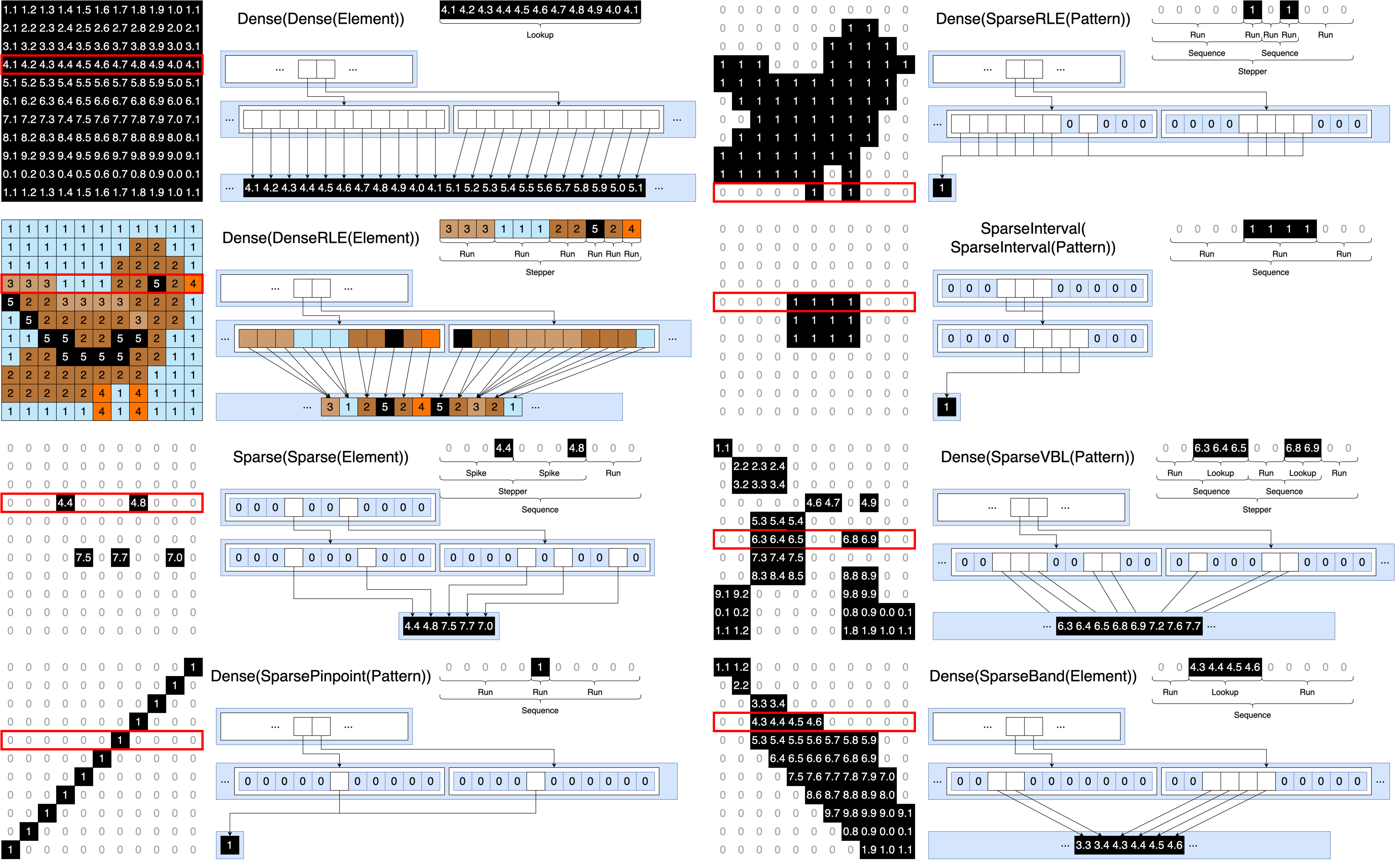
Figure 6. Several examples of matrix structures represented using the level structures identified in Table 5. Comparing this figure to (Ahrens et al., 2023, Figure 3), we see that a level-by-level structural decomposition is diagrammed together with the Looplets.

3.3. Implementations of Structures

3.3.1. Sequentially Constructed Levels

We consider all combinations of these structural properties in Table 5, resulting in 8 key level formats that correspond the the 8 resulting situations. While it is impossible to write code which precisely addresses every possible structure, our level formats can be combined to express a wide variety of hierarchical structures to a sufficient granularity that we can generate code which utilizes the four properties. For example, though banded arrays are a superset of ragged arrays, representing a ragged array using a banded format does not add much overhead. The structures we consider are exhaustive in the sense that they address all combinations of sparsity, blocks, runs, and singletons in each level. We can represent a wide variety of hierarchical tensor structures by combining these level structures in a tree, as shown in Figure 6.

3.3.2. Non-sequentially Constructed Levels

To reduce the implementation burden and improve efficiency in the common case, the levels we described in the previous section only support bulk, sequential construction of formats. However, when users want to be able to write out of order (which is a common requirement arising from loop order or from the problem itself, it occurs in our SpGEMM algorithms and our histogram example in the evaluation section), we must use more complicated datastructures like hash tables and trees to support the random writes so that in-order levels can be constructed later. Because these datastructures are more complex and have a higher implementation burden and performance overhead, we only support random access construction of sparse or dense structures. We can use these two more general structures as intermediates to convert to our more specialized structures later.

Sequentially Constructed Levels
Dense: The dense format is the simplest format, mapping $fiber(l,p)[i]\rightarrow fiber(l.lvl,p\times l.shape+i)$. This format is used to store dense data and is often a convenient format for the root level of a tensor. Due to its simplicity, freezing and thawing the level are no-ops.
DenseRLE: Used to represent runs of repeated values, storing two vectors, $right$ and $ptr$, with $q^{th}$ run in the $p^{th}$ subfiber starting and ending at $right[ptr[p]+q]$ and $right[ptr[p]+q+1]-1$, respectively. A challenge arises for this level: it is difficult to merge duplicate runs. Such a scenario might arise when merging runs of subfibers of length 3, representing colors in an image. Ideally, we would be able to detect duplicate subfibers and merge them on the fly, but we cannot determine which subfibers are equal because we cannot read them while the sublevel is in update-only mode. Instead, we merge the duplicates during the freeze phase. We $freeze$ the sublevel, $declare$ a separate sublevel $buf$ as a buffer to store the deduplicated subfibers, and then compare each of the subfibers in the main level, copying the deduplicated subfibers into the buffer.
SparseList: The simplest sparse format, used to construct popular formats like CSR, CSC, DCSR, DCSC, and CSF. It stores two vectors, $idx$ and $ptr$, such that $idx[ptr[p]+q]$ is the index of the $q^{th}$ nonzero in the subfiber at position $p$.
SparsePinpoint: Similar to SparseList, but only one nonzero in each subfiber, eliminating the need for the $ptr$ field. It stores a vector $idx$, such that $idx[p]$ is the nonzero index in the subfiber at position $p$.
SparseRLE: Similar to DenseRLE level, but because runs are sparse, we must also store the start of each run. It stores three vectors $left$, $right$, and $ptr$, such that the $q^{th}$ run in the $p^{th}$ subfiber begins and ends at $left[ptr[p]+q]$ and $right[ptr[p]+q]$, respectively. Like DenseRLE, it also stores a duplicate sublevel, $buf$, for deduplication.
SparseInterval: Similar to SparseRLE, but only stores one run per subfiber, eliminating the need for the $ptr$ field. This level does not deduplicate as it cannot store intermediate results with more than one run. It stores two vectors, such that the run in subfiber $p$ begins and ends at $left[p]$ and $right[p]$ respectively.
SparseVBL: Used to represent blocked data. It stores three vectors, $idx$, $ptr$, and $ofs$, such that $ofs[ptr[p]+q]:ofs[ptr[p]+q+1]-1$ are the subpositions of block $q$ ending at index $idx[ptr[p]+q]$ in the subfiber at position $p$.
SparseBand: Similar to SparseVBL, but stores only one block per subfiber, eliminating the need for the $ptr$ field. It stores two vectors $idx$ and $ofs$, such that $ofs[p]:ofs[p+1]-1$ are the subpositions of the block ending at $idx[p]$ in subfiber $p$.
Nonsequentially Constructed Levels
SparseHash: The sparse hash format uses a hash table to store the locations of nonzeros, and sorts the unique indices for iteration during the freeze phase. This allows for efficient random access, but not incremental construction, as the freeze phase runs in time proportional to the number of nonzeros in the entire level. It stores two vectors, $idx$ and $ptr$, such that $idx[ptr[p]+q]$ is the index of the $q^{th}$ nonzero in the subfiber at position $p$. Also stores a hash table $tbl$ for construction and random access in the level.
SparseBytemap The SparseBytemap format uses a bytemap to store which locations have been written to. Unlike the SparseHash format, the bytemap assembles the entire space of possible subfibers. This accelerates random access in the format, but requires a high memory overhead. Because we don’t want to reallocate all of the memory in each iteration, the declaration of this format instead re-assembles only the dirty locations in the tensor. This format is analogous to the default workspace format used by TACO. It stores two vectors, $idx$ and $ptr$, such that $idx[ptr[p]+q]$ is the index of the $q^{th}$ nonzero in the subfiber at position $p$. These vectors are used to collect dirty locations. It also stores $tbl$, a dense array of booleans such that $tbl[shape*p+i]$ is true when there is a nonzero at index $i$ in the subfiber at position $p$.
Leaf Levels
Element: The element level uses an array $val$ to store a value for each position $p$. The zero (fill) value is configurable.
Pattern: The pattern level statically represents a leaf level with a fill value of $false$ and whose stored values are all $true$.
Scalars
Scalar: A dense scalar that, unlike a variable, supports reduction.
SparseScalar: A scalar with a dirty bit which specializes on the fill value when it occurs.
EarlyBreakScalar: A scalar which triggers early breaks in reductions whenever an annihilator is encountered.

Table 3. The main level formats supported by Finch. Note that all non-leaf levels store a the dimension of the subfibers and a child level. Since we must be able to handle the case where a sublevel is not stored because a parent level is sparse, all of Finch’s sparse formats use a dirty bit during writing to determine whether the sublevel has been modified from it’s default fill value and thus, whether it needs to be stored.

3.3.3. Scalars

Because leaf levels are geared towards representing multiple leaves, we also introduce a much simpler Scalar format to represent 0-dimensional tensors. Scalars don’t have as much structure as clearly only two structures apply. Through these structures, scalars can also affect other tensors in crucial ways. Constant propagation through arrays is known to be a complex compiler pass (McMichen et al., [n. d.]). Instead, we provide sparse scalars, which allow reductions but also specialize read accesses for the possible zero value. We also provide early break scalars, which modify the stepper looplets to re-specialize the loop whenever a reduction into an early break scalar hits an annihilator. We don’t need to re-specialize other looplets because the stepper is the only one which repeats a non-constant number of times. We represent early break as a structural property rather than a program node because it allows us to represent the tail of a loop where one scalar has hit an annihilator but another scalar hasn’t. To our knowledge, sparse and early break scalars are novel contributions of this work; other systems don’t include them, limiting the impact of sparsity.

3.3.4. Leaf Levels

The leaf level stores the actual entries of the tensor. In most cases, it is sufficient to store each entry at a separate position in a vector. This is accomplished by the ElementLevel. However, when all of the values are the same, an additional optimization can be made by storing the identical value only once. In this work, we introduce the concept of a PatternLevel to handle this binary case. The PatternLevel has a fill value of $false$, and returning $true$ for all “stored” values. The PatternLevel allows us to easily represent unweighted graphs or other Boolean matrices.

4. The Finch Language

⬇

EXPR := LITERAL | VALUE | INDEX | VARIABLE | EXTENT | CALL | ACCESSS

STMT := ASSIGN | LOOP | DEFINE | SIEVE | BLOCK

\parDECLARE := TENSOR .= EXPR(EXPR…) #V is the set of all values

FREEZE := @freeze(TENSOR) #S is the set of all Symbols

THAW := @thaw(TENSOR) #T is the set of all types

ASSIGN := ACCESS <<EXPR>>= EXPR

LOOP := for INDEX = EXPR LITERAL := V

STMT VALUE := S::T

end TENSOR := S

DEFINE := let VARIABLE = EXPR INDEX := S

STMT VARIABLE := S

end EXTENT := EXPR : EXPR

SIEVE := if EXPR CALL := EXPR(EXPR…)

STMT ACCESS := TENSOR[EXPR…]

end MODE := @mode(TENSOR)

BLOCK := begin

STMT…

end

Figure 7. The syntax of the finch language. Compare this grammar to the Concrete Index Notation of TACO (Kjolstad et al., 2019, Figure 3), noting the addition of multiple left hand sides through code blocks, access with arbitrary expressions, and explicit declaration, as well as freeze and thaw.

4.1. Syntax

The syntax of Finch is displayed in Figure 7. The Finch syntax mirrors most imperative languages with for-loops and control flow. Notable statements that have been added to the language include

for},
\mintinline

julialet, blocks of code with

if}, and
the lifecycle functions that let us declare, freeze, and thaw tensors.
%
At the level of expressions, we support a wide array of scalar operations through literals and calls to functions whose properties and definitions are defined externally.
%
The expressions can also interact with indices and extents.
% FIXME: ???
Finally, as detailed in the previous section, tensors are defined externally via an interface that supports the $declare$, $freeze$, $thaw$, and $unfurl$ functions.
%
The first three are supported directly in the syntax whereas the four will be introduced through evaluation of \mintinline

juliafor-loops loops and accesses, in the next section. Our syntax is highly permissive: by allowing blocks of code with multiple statements, we implicitly support many features gained through complicated scheduling commands in other frameworks, such as multiple outputs, masking to avoid work, temporary tensors, and arbitrary loop fusion and nesting. These features are seen most prominently in our implementation of Gustavson’s algorithm for sparse-sparse matrix multiply, which simply writes to a temporary tensor in an inner loop and then reuses it, or in our breadth-first-search, which uses an

if} statement to avoid operating on vertices outside the frontier.
%
The only restriction we impose on our syntax is that it must respect tensor life cycles.
%
In the semantics section, we detail the specifics of how we compile our syntax to efficient code over structured data.
% Finch uses Looplets to lower \mintinline

juliafor-loops, though a sparse

4.2. Semantics

We present a sketch of a small-step operational semantics, showing how to execute a Finch program in a host language. We distinguish evaluation of the language by evolving compiler state with $\langle\rangle$ and evaluation in the host language via $\llangle\rrangle$. For example, in Figure 8, we declare the core semantics of the language and the $Define$ rule (

let}) adds a definition to the compiler state whereas the $Call$ rule passes evaluation off to the host.
%
In Figure~\ref

fig:semantics_looplets, we detail the Looplet evaluation semantics, which details how accesses within a loop can be replaced with Looplets, which are progressively rewritten to host code. Due to the use of rewrite rules, our semantics here make use of an evaluation context. We include the sketch of our semantics to highlight several key design choices. First, we note that the life cycle rules (in combination with the definition rules) prevent programs that access tensors on both the left and the right hand side of an incrementing assignment within a loop. Tensors may only change their mode in the scope in which they were declared. The loop, declare, and sieve nodes introduce new scopes, and tensors without declarations are assumed to have global scope. Beyond the simple management of iterator state, these rules allow us to effectively analyze the propagation of constants, zeros, and repetitive values within a loop, eliminating problems that in a less restrictive language would require alias analysis. Second, loops enter into a looplet system via the $Unfurl$ rule. In this system, repeated structures and constants are slowly uncovered as accesses are lowered in various points in the program (e.g. $Run$ and $Switch$, respectively). In this process, we are able to use rewrite rules in $Simplify$ to eliminate cases, unnecessary iterations, and so forth based on the information provided via Looplets and via the control flow (loops, sieve, definitions). The next section will detail how the compiler adds additional features on top of this core language. We rely on the assurance that accesses to tensor values will first unravel to Looplets and then simplify in the context of the tensor access. We will handle complex index access expressions involving indirection and arithmetic by transforming complex accesses to additional loop variables with additional tensor accesses to insert Looplets to provide the structure dictated by the complex control flow. We will also show how we can similarly exploit the structure of complex conditional expressions when the structure of the expressions is placed inside a tensor access.

⟨val, (e, t, d) ⟩→val’ var／∈d 2[$Define$]⟨define(var, val, body), (e, t, d)⟩→⟨body, (e[var ↦val’], t, {}) ⟩ ⟨args_i, (e, t) ⟩⇒vals_i ⟨f, (e, t) ⟩⇒g 2[$Call$]⟨call(f, args…), (e, t)⟩→g(vals…), t 1[$Literal$]⟨literal(val), (e, t, d)⟩→val 0[$Variable$]⟨variable(name), (e, t, d)⟩→e(variable(name)) 0[$Index$]⟨index(name), (e, t, d)⟩→e(index(name)) ⟨body, s ⟩→s’ 1[$Block$]⟨block(body, tail…), s ⟩→⟨block(tail…), s’ ⟩ 1[$Value$]⟨value(ex, type), (e, t, d)⟩⇒ex, t ⟨cond, (e, t, d) ⟩⇒true ⟨body, (e, t, {}) ⟩→(e^′, t^′, d^′) 2[$SieveTrue$]⟨sieve(cond, body), (e, t, d)⟩→(e^′, t^′, d) ⟨cond, s ⟩⇒false 1[$SieveFalse$]⟨sieve(cond, body), s⟩→s s = (e, t, d) tns／∈d e(tns) = tns’ ⟨init, s ⟩⇒init’ ∀i ⟨init, dims_i ⟩⇒dims’_i 5[$Declare$]⟨declare(tns, init, dims), s⟩→(e [mode(tns) ↦update], declare(tns’, init’, dims’…), t , d∪{ tns}) s = (e, t,d ) e(mode(tns)) = update tns∈d e(tns) = tns’ 4[$Freeze$]⟨freeze(tns), s⟩→(e [mode(tns) ↦read], freeze(tns’), t , d) s = (e, t, d) e(mode(tns)) = read tns∈d e(tns) = tns’ 4[$Thaw$]⟨thaw(tns), s⟩→(e [mode(tns) ↦update], thaw(tns’), t , d) e(tns) = tns’ ⟨op, s⟩→op’ ⟨rhs, s⟩→rhs’ [no rule]3 e(mode(tns)) = update unfurl(tns’, update, op’, rhs’), t→t’ [simple]2[$Assign$]⟨E[assign(access(tns), op, rhs)], (e, t, d)⟩→(e, t’, d)

Figure 8. Basic evaluation semantics, roughly defining most of these language constructs to function similarly to their classical definitions. The state $s$ of the finch compiler is a tuple $(e,t,d)$ of a variable value environment, another state $t$ corresponding to the state in the host language, and finally the set of tensors defined within the current scope, $d$. This means that rules which modify $t$ are running in the host language. Several looplets introduce variables into the embedding language, which may be read when evaluating the value node. All of the lifecycle functions are designed to be implemented and executed in the host language, but these semantics enforce that each of these functions may update state in the host language and flip the mode of the tensor between read and update.

$$E:=[\cdot]|\text{{loop}}(idx,ext,E|body)|\text{{block}}(E|head,E|tail)|\text{{sieve}}(E|cond,E|body)|\text{{assign}}(E|lhs,op,E|rhs)\\ \text{{declare}}(var,E|rhs,E|body)|\text{{call}}(E|f,E|args...)|\text{{access}}(tns,E|idxs...)$$

e(tns) ↦tns’ e(mode(tns)) ↦m unfurl(tns’, ext, m), t⇒tns” 3[$Unfurl$]⟨loop(i, ext, E[access(tns, j…, i)]), s⟩→⟨loop(i, ext, E[access(tns”, j…, i)]), s⟩ 0[$Run$]⟨loop(i, ext, E[access(run(body), j…, i)]), s⟩→⟨loop(i, ext, E[access(body, j…)]), s⟩ e(i) = i’ seek(i’), t →t’ 2[$Lookup$]⟨E[access(lookup(seek, body), j…, i)], (e, t, d)⟩→⟨E[access(body, j…)], (e, t’, d)⟩ 0[$AcceptRun$]⟨loop(i, extent(a, b), E[assign(access(run(body), j…, i), op, rhs)]), s⟩→⟨loop(i, extent(a, b), E[sieve(i == a, assign(access(body, j…), op, rhs))]), s⟩ cond, t ⇒true 1[]⟨E[access(switch(cond, head, tail), i…)], s⟩→⟨E[access(head, i…)], s⟩ cond, t ⇒false 1[$Switch$]⟨E[access(switch(cond, head, tail), i…)], s⟩→⟨E[access(tail, i…)], s⟩ 0[$Phase$]⟨loop(i, extent(a, b), E[access(phase(extent(c, d), body), j…, i)]), s⟩→⟨loop(i, extent(max(a, c), min(b, d)), E[access(body, j…, i)]), s⟩ preamble, t →t’ ⟨E[body], (e, t’, d) ⟩→(e’, t”, d) epilogue, t” →t”’ 3[$Thunk$]⟨E[thunk(preamble, body, epilogue)], (e, t’, d)⟩→(e’, t”’, d) ⟨loop(i, ext, E[access(head, j…, i)]), s⟩→s’ 1[$Sequence$]⟨loop(i, ext, E[access(sequence(head, tail), j…, i)]), s⟩→⟨loop(i, ext, E[access(tail, j…, i)]), s’⟩ ⟨node, algebra ⟩→node’ 1[$Simplify$]⟨E[node], s⟩→⟨E[node’], s⟩ seek(a), t →t’ 1[$StepperSeek$]⟨loop(i, extent(a, b), E[access(stepper(seek, body, next), j…, i)]), (e, t, d)⟩→⟨loop(i, extent(a, b), E[access(stepper(body, next), j…, i)]), (e, t’, d)⟩ ⟨loop(i, ext, E[access(body, j…, i)]), (e, t, d) ⟩→(e’, t’, d) next, t’ →t” 2[$StepperNext$]⟨loop(i, ext, E[access(stepper(body, next), j…, i)]), s⟩→⟨loop(i, ext, E[access(stepper(body, next), j…, i)]), (e’, t”, d)⟩ 0[$Loop$]⟨loop(i, extent(a, b), body), s⟩→⟨block(define(i, a, body), sieve(a ¡ b, loop(i, extent(a + 1, b), body))), s⟩ e(tns) ↦tns’ e(mode(tns)) ↦read unfurl(tns’, read), t→tns” 3[$Access$]⟨E[access(tns)], s⟩→⟨E[tns”], s⟩

Figure 9. Looplet evaluation semantics. Basic evaluation semantics, roughly defining most of these language constructs to function similarly to their classical definitions. The state of the compiler is described in the previous figure. Note that $E$ is an evaluation context that applies anywhere in the syntax tree. The nonlocal evaluations of Looplets are what allow Looplets to hoist conditions and subranges out of loops. However, this also means we must specify the priority in which we apply looplet rules, which is as follows: $Thunk>Phase>Switch>Simplify>Run>Spike>Sequence>StepperSeek>StepperNext>Lookup>AcceptRun>Unfurl>Loop>Access$. Many looplets, most notably the thunk looplet, introduce variables into the host language environment. While variables introduced by a looplet may be modified by the looplet itself (steppers often increment some state variables), we forbid child looplets from modifying any state variables that they didn’t introduce. This allows us to treat the value node as a constant. Note: the $Simplify$ rule references $algebra$, which is our variable defining a set of straightforward simplification rules. These rules include simple properties like $x*0\rightarrow 0$ to more complicated ones such as constant propagation. We omit the full set of rules for brevity, but point the curious reader to (Ahrens et al., 2023, Figure 5) for some examples.

5. The Finch Compiler

5.1. Finch Normal Form

Our semantics in Figure 8 and Figure 9 is only well-defined on some programs. We define a particular class of programs on which our semantics are well-defined, and refer to it as Finch Normal Form. The properties of such a program are as follows:

• Access with Indices: Though Finch allows general expressions in an access (i.e. ‘A[i + j]‘ or ‘A[I[i]]‘), the normal form restricts to allow only indices in accesses (i.e. ‘A[i]‘), rather than more general expressions.

• Evaluable Dimensions: Loop dimensions and declaration dimensions must be evaluable at the time we compile them, so we restrict the normal form to programs whose loop dimensions and declaration dimensions are extents with limits defined in the scope of the corresponding loop or declaration statement.

• Concordant: Finch is column-major by default, and the normal form requires the order of indices in an access to match the order in which loops are nested around it. For example,

  for j = _; for i = _; s[] += A[i, j] end end}
      is concordant but
      \mintinline

  julia

for i = _; for j = _; s[] += A[i, j] end end is not. Lifecycle Constraints: Tensors in read mode may appear on the right hand side only. Tensors in update mode may appear on the left hand side only. To make it easier to statically analyze lifecycle constraints, we restrict tensors to only change modes in the same scope in which they were defined. The subsequent sections will explain how programs that violate each of these constraints can be rewritten to programs that satisfy them, and thus how we can support such a wide variety of programs. For example, we can write non-concordant programs like

for i = _; for j = _; s[] += A[i, j] end end}
by adding a loop to randomly access \mintinline

juliaA or adjusting the storage order of

A} by adding a lazy transposition wrapper.
    \begin

wrapfigurer0.17

⬇

for i=_, j=_

if i <= j

s[] += A[i, j]

end

end

$\downarrow$

⬇

for i=_, j=_

if UpTriMask()[i, j]

s[] += A[i, j]

end

end

$\downarrow$

⬇

for i = 1:n

for j = 1:i

s[] += A[i, j]

end

end

Wrapperization

5.2. Wrapperization

Many fancy operations on indices can be resolved by introducing equivalent wrapper arrays which modify the behavior of the tensors they wrap, or by introducing mask arrays which replace index expressions like

i <= j} with their equivalent masks (in this case, a
    triangular mask tensor).  Wrappers and masks are summarized in \ref

tab:wrappers. All wrapper arrays are eventually unwrapped by the compiler as we lower them, some earlier than others. For example, the $swizzle$ array wraps a tensor and permutes the indices of an access when it is unwrapped during the wrapperization pass. On the other hand, the $offset$ array wraps a tensor and shifts all of the ranges declared in Figure 9 by one. The implementation burden for a wrapper is to implement a suitable program rewrite during the wrapperization procedure to unwrap the wrapper, or to implement the looplet functions of 9 with some minor modifications to shift dimensions, for example. Mask arrays have a more straightforward implementation using static looplets that are constructed during the unfurl step. Mask tensors allow us to lift computations with masks to the level of the loop, without modifying the loop directly.

Transformation Example	Description
A[i + a] $\rightarrow$ offset(A, 1)[i]	Creates an OffsetArray such that offset(tns, delta...)[i...] == tns[i .+ delta...].
A[i + x] $\rightarrow$ toeplitz(A, 1)[i, x]	Creates a ToeplitzArray, adding a dimension that shifts another dimension of the original tensor. The added dimensions are produced during a call to Unfurl, when a lookup looplet is emitted for the first dimension.
A[(a:b)(i)] $\rightarrow$ window(A, a:b)[i]	Creates a WindowedArray, representing a view into another tensor. This wrapper returns a different size of tensor.
A[ĩ] $\rightarrow$ permissive(A)[i]	Creates a PermissiveArray, allowing for out-of-bounds access or padding. This tensor returns no dimensions as its size.
A[p(i)] $\rightarrow$ swizzle(A, perm)[i]	A lazily transposed array, swizzle(A, perm)[idx…] is transformed to A[idx[perm]…] during wrapperization.
$i<j\rightarrow$ UpTriMask()[i, j - 1]	Upper triangular mask, true if $i<j$.
$i\geq j\rightarrow$ LoTriMask()[i, j]	Lower triangular mask, true if $i\geq j$.
$l\leq i<j\rightarrow$ Bandmask()[i, l, h - 1]	Banded mask, true for elements within a specified band.
$i==j\rightarrow$ DiagMask()[i, j]	Diagonal mask, true if $i==j$.
$i\neq j\rightarrow$ !(DiagMask()[i, j])	Inverse diagonal mask, true if $i\neq j$.
chunkmask(b)	Chunk mask, for chunked tensor access. True if $b\times(j-1)<i\leq b\times j$.

Table 4. Wrapper arrays, masks, and some example indexing sugar they enable.

5.3. Dimensionalization

Looplets typically require the dimension of the loop extent to match the dimensions of the tensor. However, it is cumbersome to write the dimensions in loop programs, and most tensor compilers have a means of specifying the dimensions automatically. In many pure Einsum languages like TACO, determining dimensions is not needed because any tensor dimensions that share an index are assumed to be the same (Kjolstad et al., 2017). Other languages, such as Halide, perform bounds inference where known bounds are symbolically propagated to fill in unknown bounds, often from output/input sizes to intermediates via some approximation such as interval analysis or polyhedral methods (Ragan-Kelley et al., 2013; Grosser et al., 2012). We refer to the process of discovering suitable dimensions as dimensionalization. In Finch, we use a straightforward dimensionalization algorithm on loops and declaration statements (output tensors). Finch determines the dimension of a loop index i from all of the tensors using i in an access, as well as the bounds in the loop itself, and operates similarly for declarations. Our algorithm uses the following principles, assuming dimension types form a lattice:

⬇

#A is 3 x 4

#B is 4 x 5

C .= 0

for i = 1:3

for j = _

for k = _

C[i, j] += A[i, k] * B[k, j]

end

end

end

$\downarrow$

⬇

C .= 0

for i = 1:3

for j = 1:5

for k = 1:4

C[i, j] += A[i, k] * B[k, j]

end

end

end

Figure 10. Dimensionalization.

1. We assign dimensions to indices.

2. Using an index in an access “hints” that the index should have the corresponding dimension.

3. Loop dimensions are equal to the “meet” of all hints in the loop body and any existing dimensions in the loop bounds. The meet usually asserts that dimensions match, but may also e.g. propagate info about parallelization

4. The

   _} symbol represents a dimensionless quantity at the bottom of the dimension lattice.
           \item We assign dimensions to declarations.
           \item Left hand side (updating) accesses ‘‘hint’’ the size of their tensor
           \item The dimensions of a declaration are the ‘‘meet’’ of all hints from
           the declaration to the first read.
           \item The new dimensions of the declared tensor are used when the tensor is on the right hand side (reading)
           access.
       \end

   enumerate

For example, in Figure  10, the second dimension of A must match the first dimension of B. Also, the first dimension of A must match the i loop dimension, 1:3. Finch will also resize declared tensors to match indices used in writes, so C is resized to (1:3, 1:5). If no dimensions are specified elsewhere, then Finch will use the dimension of the declared tensor.

⬇

for i = _

for j = _

s[] += A[i, j]

end

end

$\downarrow$

⬇

for i = _

for j = _

for k = _

if i == k

s[] += A[k, j]

end

end

end

end

⬇

for i = _

A[I[i]] += 1

end

$\downarrow$

⬇

for i = _

for j = _

if j == I[i]

A[j] += 1

end

end

end

Figure 11. Examples of concordization, transforming accesses to normal column major.

Dimensionalization occurs after wrapper arrays are de-sugared. You can therefore exempt a mode in an access from dimensionalization by wrapping the corresponding index in ~} to produce a "PermissiveArray" (e.g. \mintinlinejuliaA[ i]).

5.4. Concordization

After wrapperization, all arrays are normalized to column-major ordering and the unrecognized expressions are left in the access expressions. At that point, we run a pass over the code to make the program concordant. We make expressions concordant by inserting loops with one iteration. Examples are given in Figure 11.

⬇

y .= 0

for i = _

y[i] = x[i] + 1

end

for i = _

x[i] += 1

y[i] += 1

end

for i = _

x[i] += y[i]

end

$\rightarrow$ ⬇ y .= 0 for i = _ y[i] = x[i] + 1 end @thaw(x) @freeze(y) for i = _ x[i] += 1 y[i] += 1 end @freeze(x) for i = _ x[i] += y[i] end

Figure 12. Life cycle automation.

5.5. Life Cycle Automation

Finally, we introduce a pass to avoid needed to manually insert the @freeze} or \mintinlinejulia@thaw macros. The pass will insert these statements at the appropriate place in the program if they have not been inserted already, easing the burden on the programmer and bridging between structured and dense languages.

6. Case Studies

We evaluate Finch on a broad set of applications to showcase it’s efficiency, flexibility, and expressibility. All of our implementations highlight the benefits of data structure and algorithm co-design. Our implementation of sparse-sparse-matrix multiply (SpGEMM) translates classical lessons from sparse performance engineering into the language of Finch, using temporaries and randomly-accessible workspace formats to efficiently implement the three main approaches. Our study of sparse-matrix-dense-vector multiply (SpMV) highlights the benefits of precise structural specialization. Our studies of image morphology and graph applications show how Finch’s programming model can express more complex real-world kernels. Finally, we explain how flexible operators, formats, and indexing expressions in Finch have supported a flexible implementation of the Python Array API, supporting fused execution. All experiments were run on a single core of a 12-core 2-socket Intel Xeon E5-2695 v2 running at 2.40GHz with 128GB of memory. Finch is implemented in Julia v1.9, targeting LLVM through Julia. All timings are the minimum of 10,000 runs or 5s of measurement, whichever happens first. The Finch compiler is publicly available online at https://github.com/willow-ahrens/Finch.jl.

⬇

\pary .= 0

for j = _, i = _

y[i] += A[i, j] * x[j]

end

⬇

y .= 0

for j = _, i = _

y[j] += A[i, j] * x[i]

end

⬇

y .= 0

for j = _

let x_j = x[j]

y_j .= 0

for i = _

let A_ij = A[i, j]

y[i] += x_j * A_ij

y_j[] += A_ij * x[i]

end

end

#D is the diagonal

y[j] += y_j[] + D[j] * x_j

end

end

Figure 13. Finch row-major, column-major and symmetric SpMV Programs

6.1. Sparse Matrix-Vector Multiply (SpMV)

Sparse matrix-vector multiply (SpMV) has a wide range of applications and has been thoroughly studied (Liu and Vinter, 2015; Zhou et al., 2020). Because SpMV is bandwidth bound, many formats have been proposed to reduce the footprint (Langr and Tvrdík, 2016). The wide range of applications unsurprisingly results in a wide range of array structures, making it an effective kernel to demonstrate the utility of our programming model. We varied both the data formats and the SpMV algorithm. Our formats are shown in Table 14, and our programs are listed in Figure 13. In varying the program, we consider both row and column-major SpMV programs, as well as a symmetric SpMV. Finch enables us to exploit symmetry effectively. Our program restricts our attention to the canonical triangle (using masks), reuses the reads to the canonical triangle of the symmetric matrix (using a define statement), and writes the results to both relevant locations (using multiple outputs). All of our programs apply to all of our level formats, enabling exploitation of multiple structural patterns concurrently (e.g. sparsity and symmetry).

Format	Style of Matrix
Dense(SparseList(Element(0.0)))} & real, sparse \\ \mintinline[fontsize=\scriptsize] juliaDense(SparseList(Pattern()))	Boolean, sparse
Dense(SparseVBL(Element(0.0)))} & real, blocked \\ \mintinline[fontsize=\scriptsize] juliaDense(SparseBand(Element(0.0)))	real, banded

Figure 14. SpMV Tensor Formats

Figure 15 displays speedup relative to TACO, SuiteSparseGraphBLAS, and Julia’s standard library. We test using sparse matrices from a large selection of datasets spanning several previous papers: the datasets used by Vuduc et al. to test the OSKI interface (Vuduc et al., 2005), Ahrens et al. to test a variable block row format partitioning strategy (Ahrens and Boman, 2021), and Kjolstad et al. to test the TACO library (Kjolstad et al., 2017). Additionally, we included the SNAP graph collection to test with Boolean matrices. We also created some synthetic matrices containing bands of varying sizes. We tested using the row-major and column-major Finch programs in Figure 13 as well as the symmetric program where applicable; the performance displayed for Finch on each dataset is the fastest among the formats and programs we tested. For TACO, Column-major SpMV consistently performs better than row-major SpMV (an average of 1.36x better) so we use column-major SpMV in TACO as our baseline.

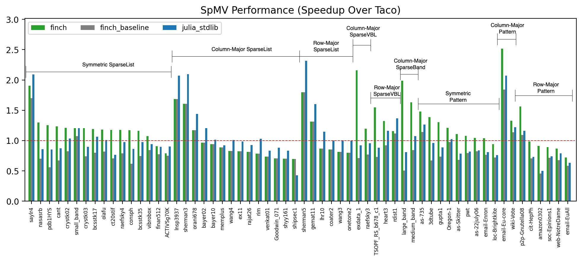
Figure 15. Performance of SpMV by Finch format. The performance displayed for Finch on each dataset is the fastest among the formats we tested. Programs are from Figure 13 and formats are from Figure 14. “finch_baseline” is the faster of row major or column major “SparseList”.

We found that the SpMV performance was superior for the level format that best paralleled the structure of the tensor. Matrices with a clear blocked structure like exdata_1, TSOPF_RS_b678_c1, and heart3 performed notably well with the SparseVBL format with speedups of 2.16, 1.55, and 1.30 relative to TACO, while the baseline format had minor slowdowns relative to TACO. Furthermore, the synthetic banded matrices we constructed performed the best with the SparseBand matrix, in particular with the large_band and the medium_band matrices having a speedup of 1.98 and 1.64 relative to TACO, while the baseline format had minor slowdowns relative to TACO. The Pattern format performed better than the Element format for representing the leaf values in the matrices when these values were Boolean, such as matrices in the SNAP collection which represent graph datasets are Boolean. For example, the SparseList-Pattern for email-Eu-core resulted in a speedup of 2.51, while the SparseList-Element format resulted in a slowdown of 1.84 over TACO. Every symmetric matrix in the SparseList and SparseList-Pattern formats has better performance when we use a Finch SpMV program that takes advantage of this symmetry. Symmetric SpMV with the SparseList level format in Finch results in an average of 1.27x speedup over TACO and symmetric SpMV with the SparseList-Pattern format in Finch results in an average speedup of 1.21x over TACO. Notably, there is a 1.91x speedup for the HB/saylr4 matrix over TACO.

6.2. Sparse-Sparse Matrix Multiply (SpGEMM)

⬇

@finch begin

C .= 0

for j=_

for i=_

for k=_

C[i, j] += AT[k, i] * B[k, j]

end

end

end

return C

end

⬇

w = Tensor(SparseByteMap(Element(0)))

@finch begin

C .= 0

for j=_

w .= 0

for k=_

for i=_

w[i] += A[i, k] * B[k, j]

end

end

for i=_

C[i, j] = w[i]

end

end

end

⬇

w = Tensor(SparseHash(SparseHash(Element(0))))

@finch begin

w .= 0

for k=_

for j=_

for i=_

w[i, j] += A[i, k] * BT[j, k]

end

end

end

C .= 0

for j=_, i=_

C[i, j] = w[i, j]

end

end

Figure 16. Inner Products, Gustavson’s, and Outer Products matrix multiply in Finch

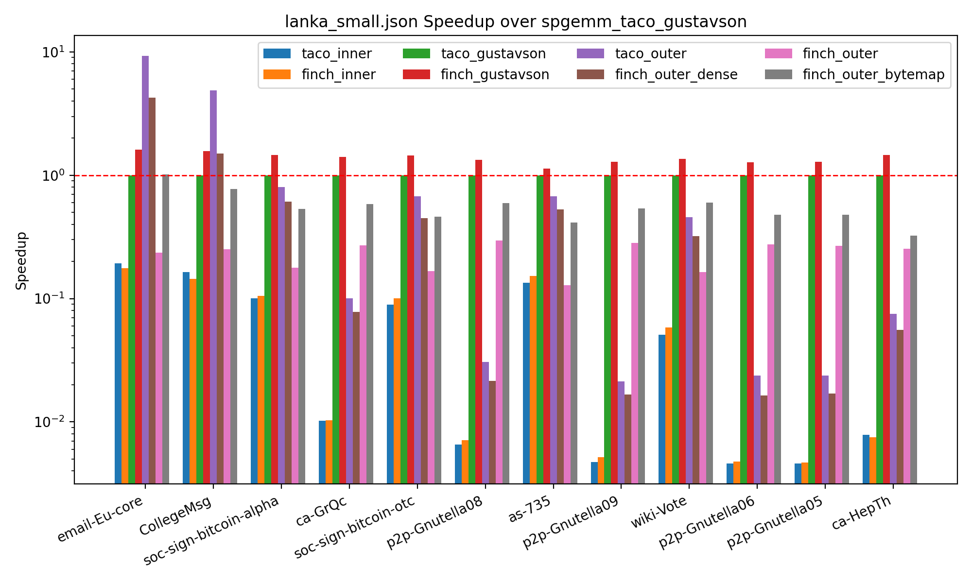
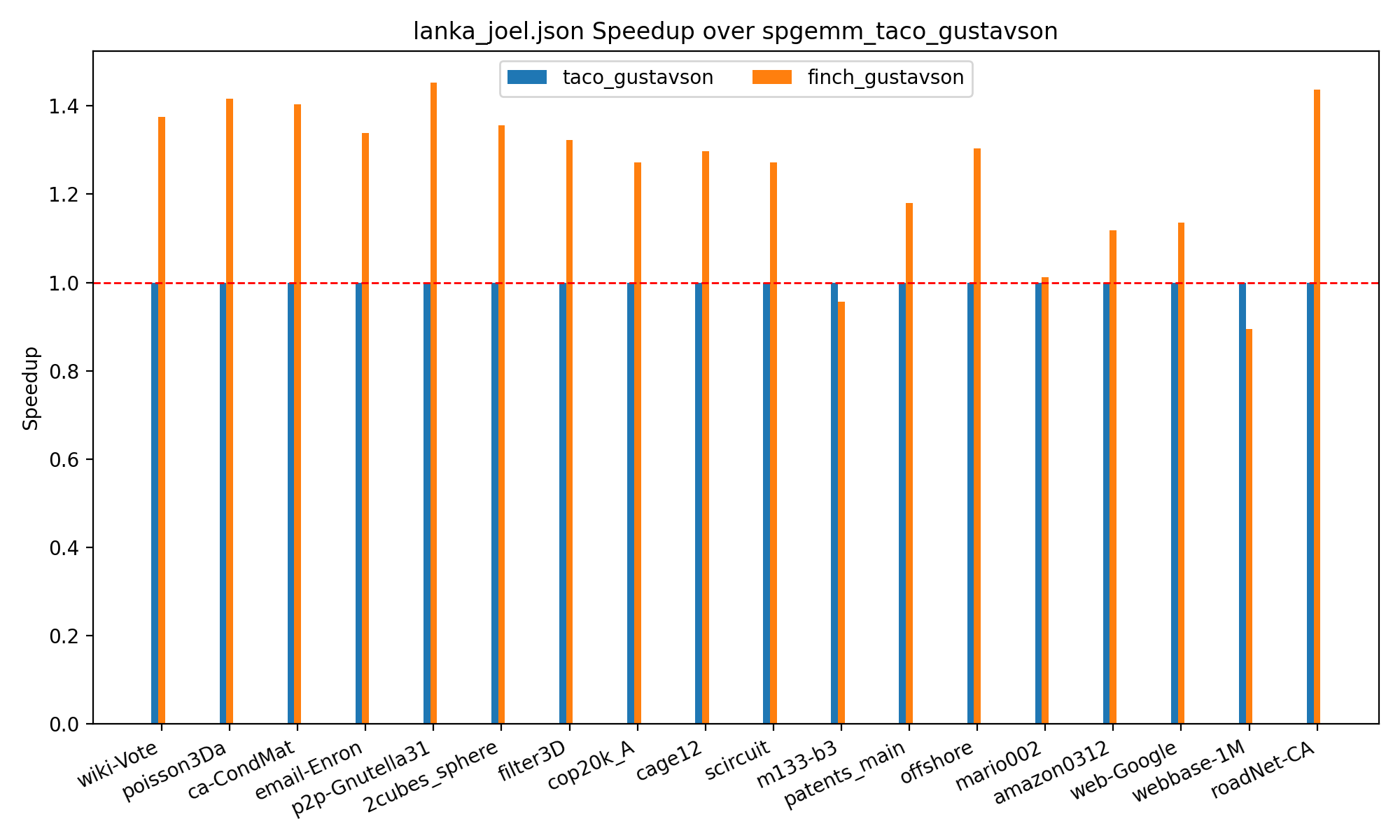
Figure 17. A comparison of several matrix multiply algorithms between Finch and Taco. On left, we use smaller matrices, ordered from small to big dimension. Note that inner-products necessarily requires $O(MN)$ work and TACO’s outer-products format is dense. Finch can use a sparse outer products format and thus has an asymptotic advantage that becomes evident as the output dimensions grow. On right, we use only Gustavson’s algorithm and compare on larger matrices.

We compute the $M\times N$ sparse matrix $C$ as the product of $M\times K$ and $K\times N$ sparse matrices $A$ and $B$. There are three main approaches to SpGEMM (Zhang et al., 2021, Section 2.2). The inner-products algorithm takes dot products of corresponding rows and columns, while the outer-products algorithm sums the outer products of corresponding columns and rows. Gustavson’s algorithm sums the rows of $B$ scaled by the corresponding nonzero columns in each row of $A$. Inner-products is known to be asymptotically less efficient than the others, as we must do a merge operation to compute each of the $O(MN)$ entries in the output (Ahrens et al., 2022). We will show that our ability to implement these latter methods exceeds that of TACO, translating to asymptotic benefits. Figure 16 implements all three approaches in Finch, and Figure 17 compares the performance of Finch to TACO. Note that these algorithms mainly differ in their loop order, but that different data structures can be used to support the various access patterns induced. In our Finch implementation of outer products, we use a sparse hash table, as it is fully-sparse and randomly accessible. Since, TACO does not support multidimensional sparse workspaces, its outer products uses a dense intermediate, which leads to an asymptotic slow down shown in Figure 17. Similarly, although a sparse bytemap has a dense memory footprint, we use it in our Finch implementation of Gustavson’s for the smaller $O(N)$ intermediate. We note that the bytemap format in TACO’s Gustavson’s implementation is hard-wired, whereas Finch’s programming model allows us to write algorithms with explicit temporaries and transpositions. Without such hard wiring, TACO would have to use a dense intermediate to support random writes, which TACO would then propagate to the output, turning it dense and leading to the same asymptotic results as in the case of outer products. As depicted in Figure 17, Finch achieves comparable performance with TACO on smaller matrices when we use the same datastructures, and significant improvements when we use better datastructures. Finch outperforms TACO on larger matrices, with an average speedup of 1.25.

6.3. Graph Analytics

We used Finch to implement both Breadth-first search (BFS) and Bellman-Ford single-source shortest path. Our BFS implementation and graphs datasets are taken from Yang et al. (Yang et al., 2018), including both road networks and scale-free graphs (bounded node degree vs. power law node degree). Direction-optimization (Beamer et al., 2012) is crucial for achieving high BFS performance in such scenarios, switching between push and pull traversals to efficiently explore graphs. Push traversal visits the neighbors of each frontier node, while pull traversal visits every node and checks to see if it has a neighbor in the frontier. The advantage of pull traversal is that we may terminate our search once we find a node in the frontier, saving time in the event the push traversal were to visit most of the graph anyway. Early break is the critical part of control flow in this algorithm, though the algorithms also require different loop orders, multiple outputs, and custom operators. Figure 19 compares performance to Graphs.jl, a Julia library, and the LAGraph Library, which implements graph algorithms with sparse linear algebra using GraphBLAS (Mattson et al., 2019). For the BFS algorithm, direction-optimization notably enhances performance for scale-free graphs. Although GraphBLAS uses hardwired optimizations, Finch is competitive. On Bellman-Ford (with path lengths and shortest-path tree), Finch’s support for multiple outputs, sparse inputs, and masks leads to superior performance over GraphBLAS (average speedup of 3.53). We did not include GAP-road as it timed out. In Appendix B, we display the code for BFS and Bellman-Ford in Finch (57 and 50 LOC) and LAGraph (215 and 227 LOC), and invite readers to compare the clarity of the algorithms.

⬇

V = Tensor(Dense(Element(false)))

P = Tensor(Dense(Element(0)))

F = Tensor(SparseByteMap(Pattern()))

_F = Tensor(SparseByteMap(Pattern()))

A = Tensor(Dense(SparseList(Pattern())))

AT = Tensor(Dense(SparseList(Pattern())))

\parfunction bfs_push(_F, F, A, V, P)

@finch begin

_F .= false

for j=_, k=_

if F[j] && A[k, j] && !(V[k])

_F[k] |= true

P[k] <<choose(0)>>= j

end

end

return _F

end

end

\par

⬇

function bfs_pull(_F, F, AT, V, P)

p = ShortCircuitScalar{0}()

@finch begin

_F .= false

for k=_

if !V[k]

p .= 0

for j=_

if F[follow(j)] && AT[j, k]

p[] <<choose(0)>>= j

end

end

if p[] != 0

_F[k] |= true

P[k] = p[]

end

end

end

return _F

end

end

⬇

_D = Tensor(Dense(Element(Inf)), n)

D = Tensor(Dense(Element(Inf)), n)

function bellmanford(A, _D, D, _F, F)

@finch begin

F .= false

for j = _

if _F[j]

for i = _

let d = _D[j] + A[i, j]

D[i] <<min>>= d

F[i] |= d < _D[i]

end

end

end

end

end

Figure 18. Graph Applications written in Finch. Note that parents are calculated separately for Bellman-Ford. The $choose(z)$ operator is a GraphBLAS concept which returns any argument that is not $z$.

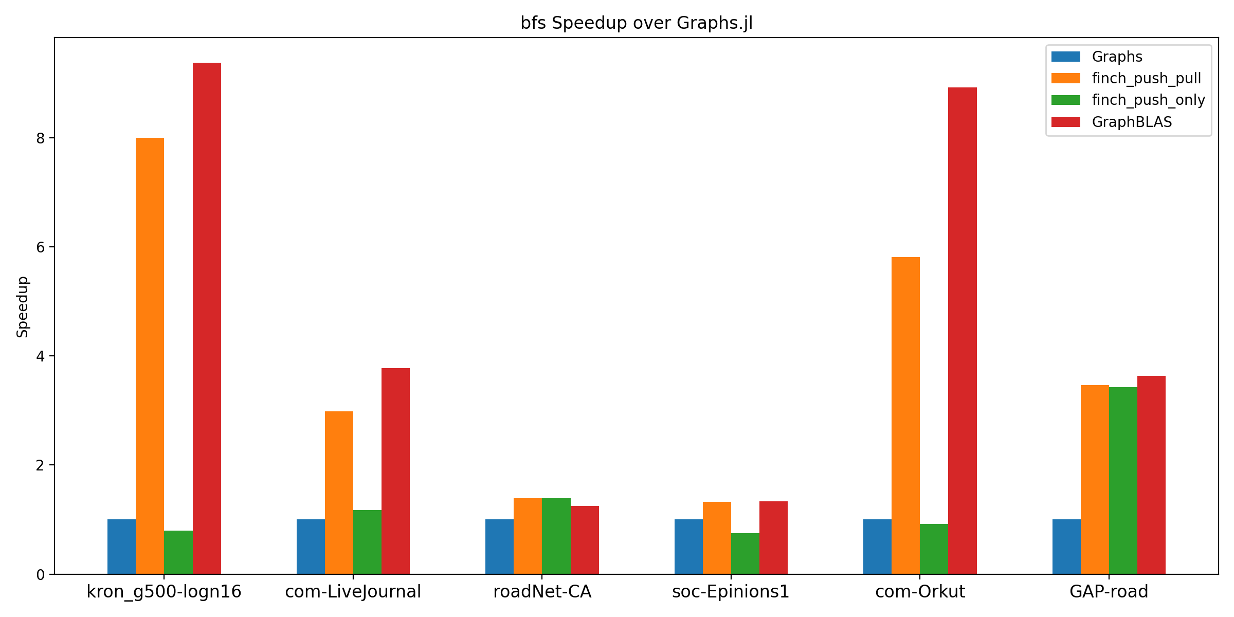
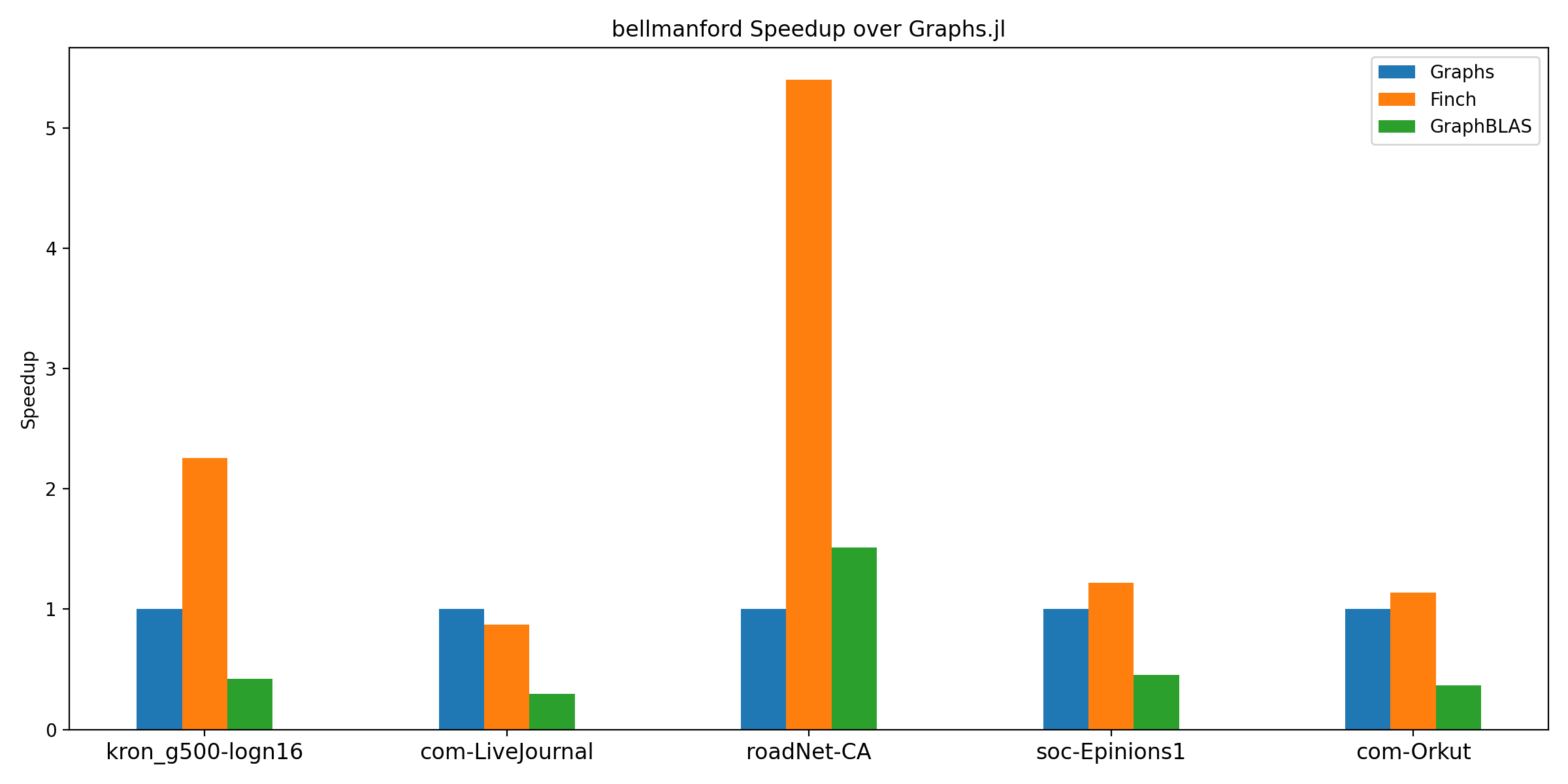
Figure 19. Performance of graph apps across various tools. finch_push_only exclusively utilizes push traversal, while finch_push_pull applies direction-optimization akin to GraphBLAS. Finch’s support for push/pull traversal and early break facilitates direction-optimization. Among GraphBLAS’s five variants for Bellman-Ford, we selected LAGraph_BF_full1a, consistently the fastest with our graphs.

6.4. Image Morphology

Some image processing pipelines stand to benefit from structured data processing (Donenfeld et al., 2022). We focus on binary image morphology and the logical transformation of binary images and masks. We consider two operations: binary erosion (computing a mask), and a masked histogram (using a mask to avoid work). We use images are all binary, either by design or having been thresholded. Finch allows us choose our datastructure, so we may choose to use either a dense representation with bytes ($Dense(Element(0x00))$), a bit-packed representation ($Dense(Element(UInt64))$), or a run-length encoded representation that represents runs of true or false ($SparseRLE(Pattern())$). All of these have their advantages. The dense representation induces the least overhead, the bit-packed representation can take advantage of bitwise binary ops, and the run-length encoded version only uses memory and compute when the pattern changes. Similarly, since Finch let’s us choose our algorithm we can implement erosion in a few ways. The erosion operation turns off a pixel unless all of it’s neighbors are on. This can be used to shrink the boundaries of a mask, and remove point instances of noise (Fisher et al., 1996). This introduces three instances of structure in the control flow: the mask, the padding of inputs, and the convolutional filter. We focused on the filter. We might understand the filter as a structured tensor of circular shifts, or we might understand each shifted view of the data in an unrolled stencil computation as a structured tensor, or a two part stencil where we compute the horizontal then vertical part of the stencil. We experimented with these options and found that the last approach performed best, due to fitting the storage formats while reducing the amount of work with intermediate temporaries. Figure 20 displays example erosion algorithms for bitwise or run-length-encoded algorithms. We compared against OpenCV. We used four datasets. We randomly selected 100 images from the MNIST (Lecun et al., 1998) and Omniglot (Lake et al., 2015) character recognition datasets, as well as a dataset of human line drawings (Eitz et al., 2012). We also hand-selected a subset of mask images (these images were less homogeneous, so we listed them in Appendix C) from a digital image processing textbook (Gonzalez and Woods, 2006). All images were thresholded, and we also include versions of the images that have been magnified before thresholding, to induce larger constant regions. In our erosion task, the SparseRLE format performs the best as it is asymptotically faster and uses less memory, leading to a 19.5X speedup over OpenCV on the sketches dataset, which becomes arbitrarily large as we magnify the images (here shown as 266X). We believe the 51.6x on MNIST is due to calling overhead in OpenCV. The bitwise kernels were effective as well, and would be more effective on datasets with less structure. A strength of Finch is that it supports structured datasets, even over bitwise operations, allowing us to implement the bitwise kernel and then mask it. We also implemented a histogram kernel. We used an indirect access into the output to implement this (Figure 20), something not many sparse frameworks support. We compare to OpenCV since the OpenCV histogram function also accepts a mask. If we use $SparseRLE(Pattern())$ for our mask, we can reduce the branching in the masked kernel and get better performance. The improvements with SparseRLE are seen in the histogram task too, as it allows us to mask off contiguous regions of computation, instead of individual pixels, reducing the branches and leading to a significant speedup (20.3x on Omniglot and 20.8x on sketches).

Wordwise Erosion:

⬇

output .= false

for y = _

tmp .= false

for x = _

tmp[x] = coalesce(input[x, ~(y-1)], true) & input[x, y] & coalesce(input[x, ~(y+1)], true)

end

for x = _

output[x, y] = coalesce(tmp[~(x-1)], true) & tmp[x] & coalesce(tmp[~(x+1)], true)

end

end

Masked Histogram:

⬇

bins .= 0

for x=_

for y=_

if mask[y, x]

bins[div(img[y, x], 16) + 1] += 1

end

end

end

Bitwise Erosion:

⬇

output .= 0

for y = _

tmp .= 0

for x = _

if mask[x, y]

tmp[x] = coalesce(input[x, ~(y-1)], 0xFFFFFFFF) & input[x, y] & coalesce(input[x, ~(y+1)], 0xFFFFFFFF)

end

end

for x = _

if mask[x, y]

let tl = coalesce(tmp[~(x-1)], 0xFFFFFFFF), t = tmp[x], tr = coalesce(tmp[~(x+1)], 0xFFFFFFFF)

let res = ((tr << (8 * sizeof(UInt) - 1)) | (t >> 1)) & t & ((t << 1) | (tl >> (8 * sizeof(UInt) - 1)))

output[x, y] = res

end

end

end

end

end

Figure 20. Two approaches to erosion in Finch. The $coalesce$ function defines the out of bounds value. On left, the naive approach. On $SparseRLE(Pattern())$ inputs, this only performs operations at the boundaries of constant regions. On right, a bitwise approach, using a mask to limit work to nonzero blocks of bits.

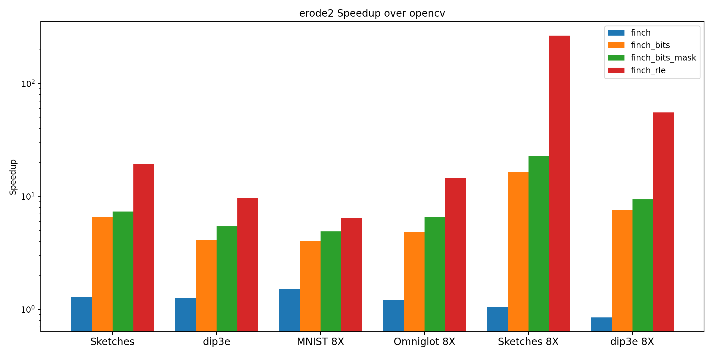
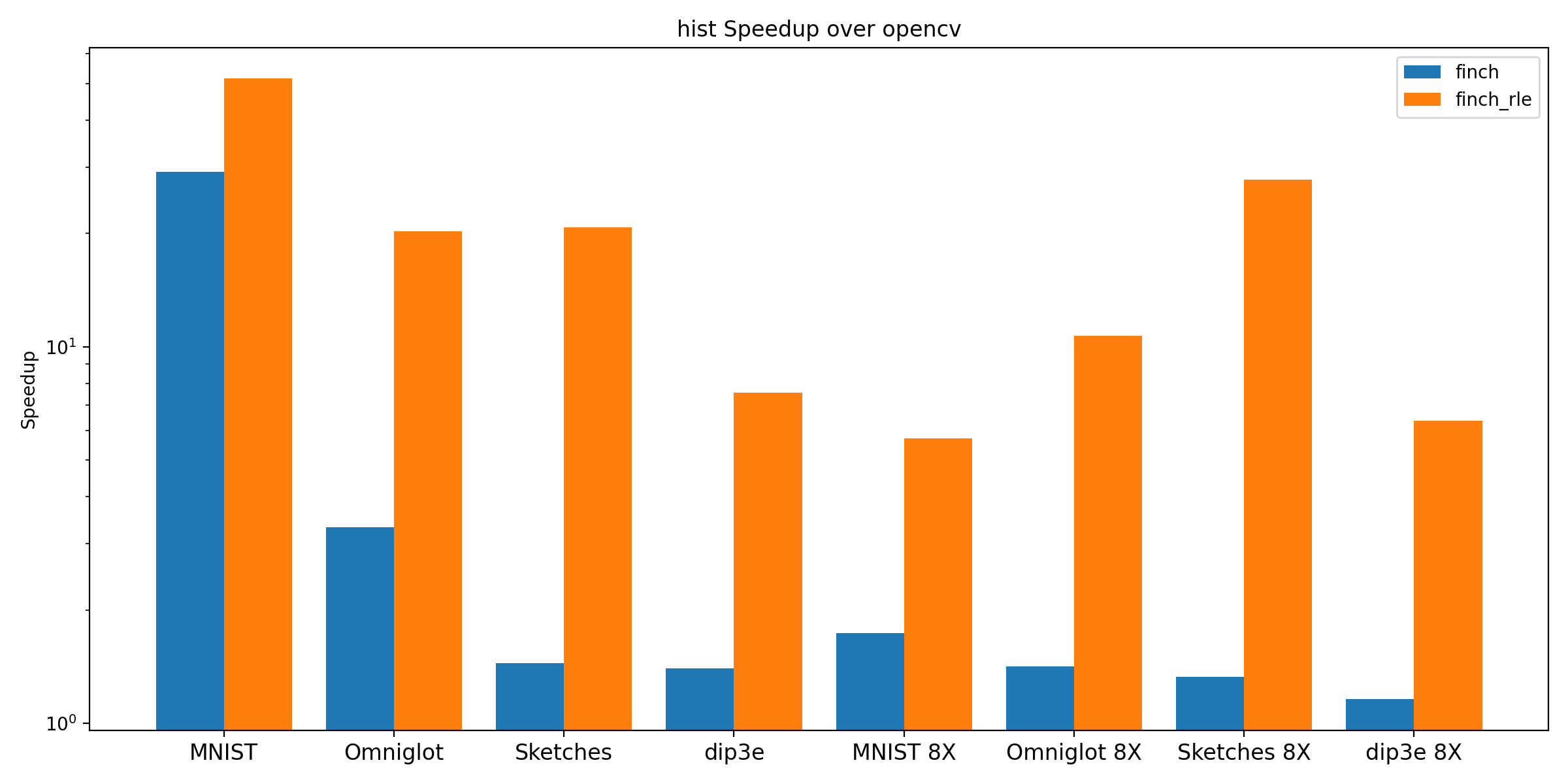
Figure 21. Performance of Finch on image morphology tasks. On left, we run 2 iterations of erosion. On right, we run a masked histogram.

6.5. Implementing NumPy’s Array API in Finch

In the past decade, the adoption of the Python Array API (Harris et al., 2020) has allowed for a proliferation array programming systems, but existing implementations of this and similar APIs for structured data suffer from either incompleteness or inefficiency. These APIs have hundreds of required functions, from mapreduce to slicing and windowing. Compilers with simpler interfaces (such as TACO’s simple Einsum) need a massive amount of glue code outside of the normal compilation path to support the full API, leading to a large implementation burden. As the API’s were designed for only one structure (Dense), the burden only grows with the introduction of as additional structures such as sparsity, as these structures interact with the complex interface and with each other. Further, implementing each operation on its own is insufficient. Operator fusion is required to avoid asymptotic performance degradation on sparse kernels, as we show in Figure 24. A flexible compiler like Finch, which can produce efficient code for arbitrary operations between inputs in a wide variety of formats, is the missing piece needed to implement the full array API for structured data with competitive performance. To handle the expansiveness of the Array API while preserving opportunities for fusion and whole workflow optimization, we pursued a lazy evaluation strategy mediated by a high-level query language. This is implemented by 1) Finch Logic, a minimal, high-level language for expressing array operations and 2) the Physical Interpreter, which executes Finch Logic as a sequence of Finch programs.

⬇

EXPR := table(TENSOR, FIELDS…) | #TENSOR is a tensor value

ALIAS | FIELD | mapjoin(OP, EXPRS…) | #OP is a function

aggregate(OP, INIT, EXPR, FIELDS…) | #INIT is an initial value

reorder(EXPR, FIELDS…) | #FIELD is a name for an index

relabel(EXPR, FIELDS…) | #ALIAS is a name for a tensor

reformat(TENSOR, EXPR) PLAN := plan(QUERIES…)

QUERY := query(ALIAS, EXPR)

Figure 22. Finch Logic Syntax.

⬇

sum(A, dims=2) = aggregate(+, relabel(A, i_1, …, i_d), i_2)

matmul(A, dims=2) = aggregate(+, mapjoin(*, relabel(A, i, j), relabel(B, j, k)))

argmin(A) = aggregate(minby, (Inf, len(A)), mapjoin(tuple, relabel(A, i), i), i)

norm2(A) = aggregate(scaled_plus, (0, 0), mapjoin(tuple, mapjoin(sign, A), mapjoin(abs, A)), fields(A)…)

where(C, A, B) = mapjoin(ifelse, relabel(C, i), relabel(A, i), relabel(B, i))

slice(A, i:j) = table(WindowedArray(A, i:j), k)

cat(A, B) = mapjoin(coalesce, table(PermissiveArray(A), i), table(OffsetArray(B, length(A)), i))

Figure 23. Implementations of a few common functions in Finch Logic. Here, minby(x, y) compares x[1] and y[1] and returns the smaller x or y. scaled_plus rescales whichever argument is smaller, then adds the values with the same scale. ifelse(c, a, b) returns a when c is true, b otherwise. Finch can understand declared properties and rewrite rules for all of these functions and types, extending these algorithms to operate on structured arguments.

6.5.1. Finch Logic and the Physical Interpreter

Finch Logic is used as a common representation to implement and fuse the operations in the Array API. The syntax is designed to be minimal and expressive, taking inspiration from relational algebra with the goal of being able to express most of the operations in the Array API.

Finch Logic

The syntax of Finch Logic is described in Figure 22. Our mapjoin represents pointwise application, while aggregate represents reductions. We name the result of each computation with query, and join several expressions in a plan. reorder reorders the indices while relabel relabels them. reformat hints at materialization into its argument. Finch’s support for arbitrary user-defined functions allows us to support complex operations such as argmin}, \mintinlinepythonnorm, and where}, all over structured data. Finch’s support for wrapper arrays allows us to express indexing operations. These situations are shown in Figure~\reffig:api_extensible.

Heuristic Optimization

Once we express our operation in Finch Logic, we use a quick heuristic to fuse the expressions. We heuristically split nested aggregate queries into separate queries, and fuse all of the mapjoins into corresponding aggregates. We then heuristically choose a loop order for each query with reorder nodes, and introduce separate query nodes to transpose so that the resulting expressions are concordant. Our heuristic assigns a format to each output by recursively evaluating the properties of structure (sparsity, repetition, etc.) and checking whether they are preserved under the operation in question.

Finch Interpreter

Once the program is in a standard form where each query has a specified format with reformat and at most one aggregate, the Finch Interpreter executes each query, in order, through a straightforward lowering process.

6.5.2. Evaluation

To demonstrate the performance of our array implementation, we evaluate it on 1) triangle counting 2) SDDMM 3) and element-wise operations. Further, we compare against DuckDB as a state of the art system which implements a form of kernel fusion through pipelined query execution. To do this, we express each of these kernels as a single select, join, groupby query. For the element-wise case, we provide an unfused Finch method to show the impact of fusion. For triangle counting, we use the same set of graph matrices as in Figure 19. For SDDMM, we use this set of graph matrices for the sparse matrix, and we produce random dense matrices with embedding dimension 25. Lastly, for the elementwise operations, we use uniformly sparse matrices with dimension 10000 by 10000. A/B have sparsity $.1$, and we vary the sparsity of C in the X axis. Across all three of these kernels, we see that the high level interface for Finch provides a major improvement over DuckDB, ranging from $1.2x-28x$. For triangle counting and SDDMM, this improvement stems from Finch’s efficient intersection of the nonzero indices as opposed to DuckDB’s use of binary join plans. For element-wise operations, this improvement stems from Finch’s better handling of expressions which combine index intersection and union and its compressed data representation.

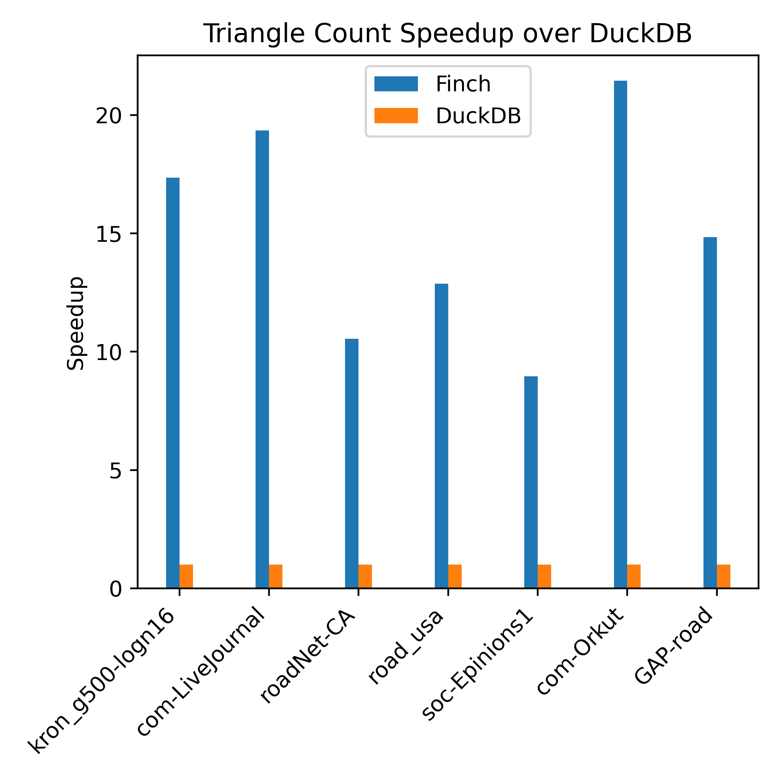
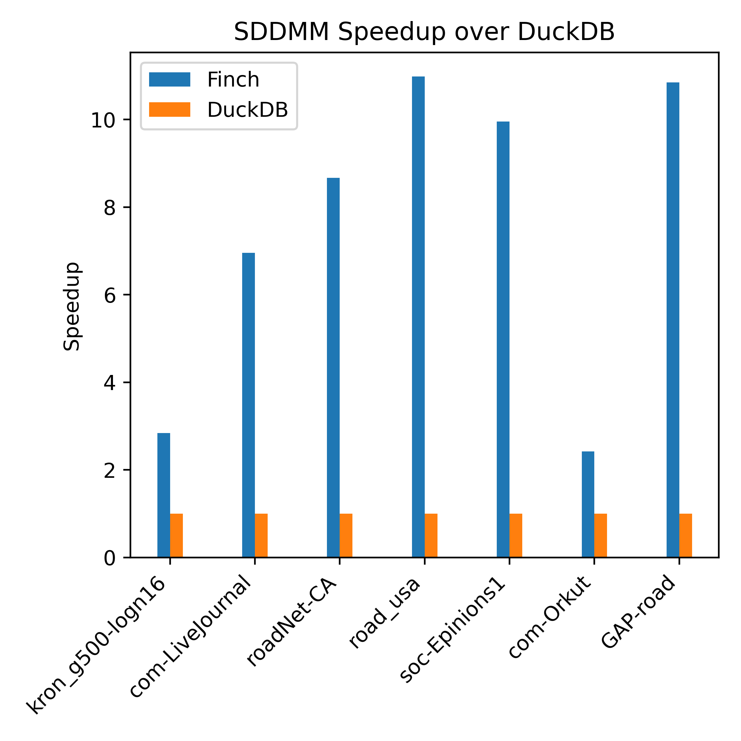
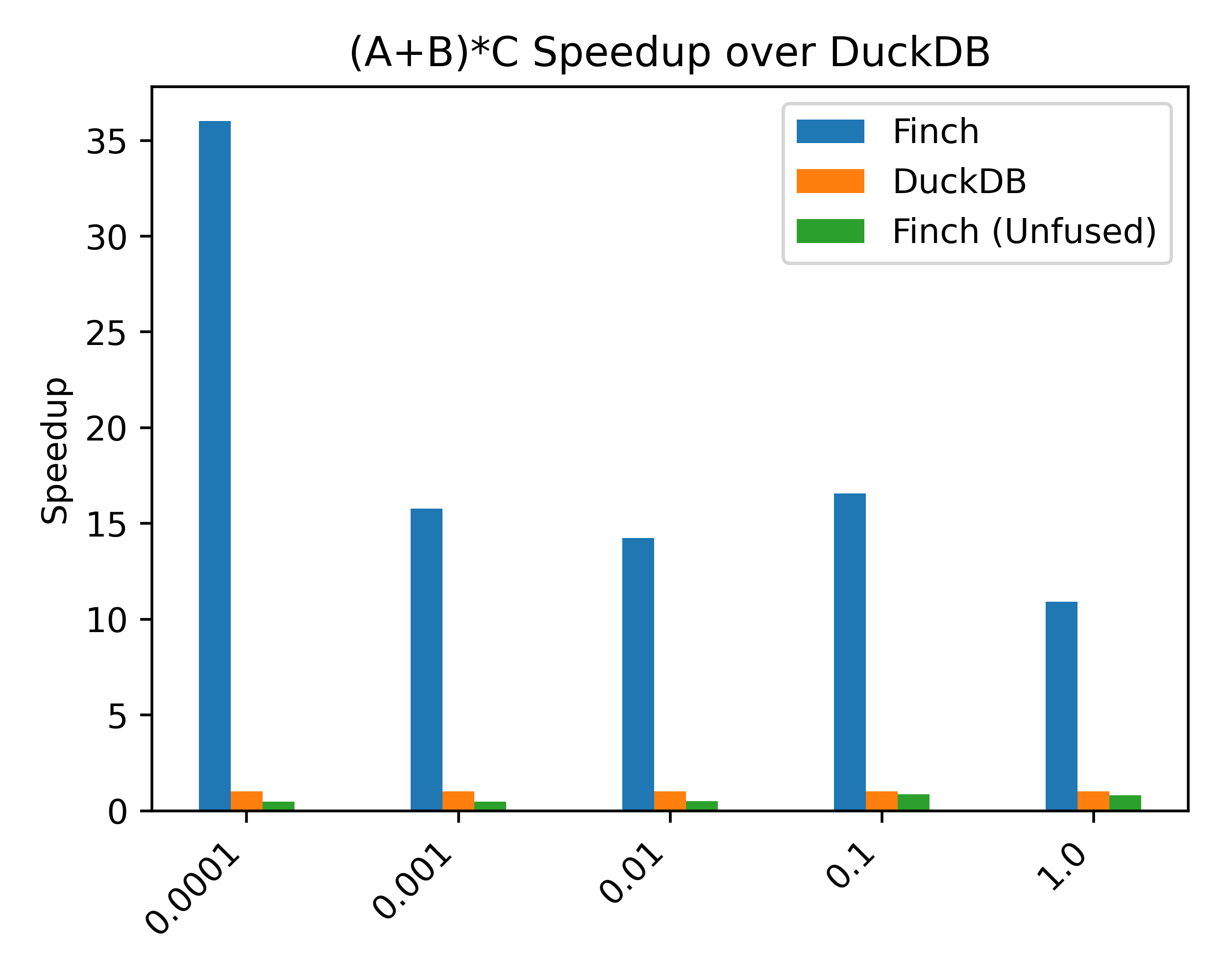
Figure 24. Performance of Finch Logic for common kernels.

7. Related Work

The related work on array languages and libraries spans several areas, from libraries to languages, from dense to structured computation.

Libraries for Dense Data:

Many libraries specialize in dense computations. Perhaps the most well-known example is NumPy (Harris et al., 2020), and a classic example is the BLAS, though several BLAS routines are specialized to symmetric, hermitian, and triangular matrices (Anderson et al., 1999). Many research projects have advanced on BLAS, such as BatchedBlas and BLIS (Dongarra et al., 2017; Van Zee and van de Geijn, 2015).

Libraries for Structured Data:

Many libraries support BLAS plus a few sparse array types, typically CSR, CSC, BCSR, Banded, and COO. Examples include SciPy (Virtanen et al., 2020), PETSc (ABHYANKAR et al., [n. d.]), Armadillo (Rumengan et al., 2021), OSKI (Vuduc et al., 2005), Cyclops (Solomonik et al., 2013), MKL (noa, 2024), and Eigen (Guennebaud et al., 2010). There are even libraries for very specific kernels and format combinations, such as SPLATT (Smith et al., 2015) (MTTKRP on CSF). Several of these libraries also feature some graph or mesh algorithms built on sparse matrices. The GraphBLAS (Kepner et al., 2016) supports primitive semiring operations (operations beyond $(+,*)$, such as $(min,+)$ multiplication) which can be composed to enable graph algorithms, some of which are collected in LAGraph (Mattson et al., 2019). Similarly, the MapReduce and Hadoop platforms support operations on indexed collections (Dean and Ghemawat, 2008), and have been used to support graph algorithms in the GBASE library(Kang et al., 2011). Several machine learning frameworks support some sparse arrays and operations, most notably TorchSparse(Tang et al., 2022, 2023).

Compilers for Dense Data:

Outside of general purpose compilers, many compilers have been developed for optimizing dense data on a variety of control flow. Perhaps the most well known example is Halide (Ragan-Kelley et al., 2013) and its various descendant such as TVM (Chen et al., 2018), Exo (Ikarashi et al., 2022), Elevate (Hagedorn et al., 2020), and ATL (Liu et al., 2022). These languages typically support most control flow except for an early break though some don’t support arbitrary reading/writing or even indirect accesses. Several polyhedral languages, such as Polly (Grosser et al., 2012), Tiramisu (Baghdadi et al., 2019), CHiLL (Chen et al., 2008), Pluto (Bondhugula et al., 2008), and AlphaZ (Yuki et al., 2012) offer similar capabilities in terms of control flow though they often support more irregular regions that the polyhedral framework supports. These are based on ISL (Verdoolaege, 2010). The density of this research represents the density of support for dense computation.

Compilers for Structured Data:

Several compilers exist for several types of structured data, often featuring separate languages for the storage of the structured data and the computation. The TACO compiler originally supported just plain Einsum computations (Kjolstad et al., 2017), but has been extended several times to support (single dimensional) local tensors (Kjolstad et al., 2019), imperfectly nested loops (Dias et al., 2022), breaks via semi-rings (Henry et al., 2021), windowing and tiling (Senanayake et al., 2020), and convolution (Won et al., 2023), and compilation in MLIR (Bik et al., 2022), all as separate extensions. Similarly, TACO originally support just dense and CSF like N dimensional structures, but was extended independently to support COO like structures (Chou et al., 2018), and tree like structures (Chou and Amarasinghe, 2022), as separate extensions. SparseTIR is a similar system supporting combined sparse formats (including block structures) (Ye et al., 2023). The SDQL language offers a similar level of control flow (Shaikhha et al., 2022), but only on sparse hash tables. Similarly, SDQL has been extended with a system that allows one to specify formats as queries on a set of base storage types (Schleich et al., 2023) and separately by another system that describes static symmetries and other structures as predicates (Ghorbani et al., 2023). The Taichi language focuses on a single sparse data structure made from dense blocks, bit-masks, and pointers (Hu et al., 2019). The sparse polyhedral framework builds on CHiLL for the purpose of generating inspector/executor optimizations (Strout et al., 2018) though the branch of this work that specifies sparse formats separately from the computation (otherwise they are inlined into the computation manually) seems to apply mainly to Einsums (Zhao et al., 2022). Second to last, SQL’s classical physical/logical distinction is the classic program/format distinction, and SQL supports a huge variety of control flow constructs (Kotlyar et al., 1997; Date, 1989). However, many SQL or dataframe systems rely on b-trees, columnar, or hash tables, with only a few systems, such as Vectorwise (Boncz and Zukowski, 2012), LaraDB (Hutchison et al., 2017), GMAP (Tsatalos et al., 1996), or SciDB (Stonebraker et al., 2013) building physical layouts with other constructs based in array programming. However, array based databases are a new focus given the rise of mixed ML/DB pipelines (Baumann et al., 2021; Luo et al., 2018). Lastly, SPIRAL focuses on recursively defined datastructures and recursively define linear algebra, and can therefore express a structure and computation that none of the systems mentioned above can: a Cooley–Tukey FFT  (Franchetti et al., 2018, 2009).

Other Architectures:

Sparse compilers have been extended to many architectures. An extension of TACO supports GPU (Senanayake et al., 2020), Cyclops (Solomonik et al., 2013; Solomonik and Hoefler, 2015) and SPDistal (Yadav et al., 2022) support distributed memory, and the Sparse Abstract Machine (Hsu et al., 2023) supports custom hardware. We believe that supporting control flow is the first step towards architectural support beyond unstructured sparsity.

8. Conclusion

Finch automatically specializes flexible control flow to diverse data structures, facilitating productive algorithmic exploration, flexible array programming, and efficient high-level interfaces for a wider variety of applications than ever before.

- (1)
- noa (2024) 2024. Developer Reference for Intel® oneAPI Math Kernel Library for Fortran. (April 2024). https://www.intel.com/content/www/us/en/docs/onemkl/developer-reference-fortran/2024-0/overview.html
- Abadi et al. (2016) Martin Abadi, Paul Barham, Jianmin Chen, Zhifeng Chen, Andy Davis, Jeffrey Dean, Matthieu Devin, Sanjay Ghemawat, Geoffrey Irving, Michael Isard, Manjunath Kudlur, Josh Levenberg, Rajat Monga, Sherry Moore, Derek G. Murray, Benoit Steiner, Paul Tucker, Vijay Vasudevan, Pete Warden, Martin Wicke, Yuan Yu, and Xiaoqiang Zheng. 2016. TensorFlow: A system for large-scale machine learning. In 12th USENIX Symposium on Operating Systems Design and Implementation (OSDI 16). 265–283. https://www.usenix.org/system/files/conference/osdi16/osdi16-abadi.pdf
- Abbasi (2023) Hameer Abbasi. 2023. Plans for new sparse compilation backend · pydata/sparse · Discussion #618. https://github.com/pydata/sparse/discussions/618
- Abelson and Sussman (1996) Harold Abelson and Gerald Jay Sussman. 1996. Structure and Interpretation of Computer Programs. The MIT Press. https://library.oapen.org/handle/20.500.12657/26092 Accepted: 2019-01-17 23:55.
- ABHYANKAR et al. ([n. d.]) SHRIRANG ABHYANKAR, GETNET BETRIE, DANIEL A MALDONADO, LOIS C MCINNES, BARRY SMITH, and HONG ZHANG. [n. d.]. PETSc DMNetwork: A Scalable Network PDE-Based Multiphysics Simulator. ([n. d.]).
- Ahrens and Boman (2021) Willow Ahrens and Erik G. Boman. 2021. On Optimal Partitioning For Sparse Matrices In Variable Block Row Format. https://doi.org/10.48550/arXiv.2005.12414 arXiv:2005.12414 [cs].
- Ahrens et al. (2023) Willow Ahrens, Daniel Donenfeld, Fredrik Kjolstad, and Saman Amarasinghe. 2023. Looplets: A Language for Structured Coiteration. In Proceedings of the 21st ACM/IEEE International Symposium on Code Generation and Optimization (CGO 2023). Association for Computing Machinery, New York, NY, USA, 41–54. https://doi.org/10.1145/3579990.3580020
- Ahrens et al. (2022) Willow Ahrens, Fredrik Kjolstad, and Saman Amarasinghe. 2022. Autoscheduling for sparse tensor algebra with an asymptotic cost model. In Proceedings of the 43rd ACM SIGPLAN International Conference on Programming Language Design and Implementation (PLDI 2022). Association for Computing Machinery, New York, NY, USA, 269–285. https://doi.org/10.1145/3519939.3523442
- Anderson et al. (1999) E. Anderson, Z. Bai, C. Bischof, L. S. Blackford, J. Demmel, J. Dongarra, J. Du Croz, A. Greenbaum, S. Hammarling, A. McKenney, and D. Sorensen. 1999. LAPACK Users’ Guide. Society for Industrial and Applied Mathematics. https://doi.org/10.1137/1.9780898719604
- Backus et al. (1957) J. W. Backus, R. J. Beeber, S. Best, R. Goldberg, L. M. Haibt, H. L. Herrick, R. A. Nelson, D. Sayre, P. B. Sheridan, H. Stern, I. Ziller, R. A. Hughes, and R. Nutt. 1957. The FORTRAN automatic coding system. In Papers presented at the February 26-28, 1957, western joint computer conference: Techniques for reliability (IRE-AIEE-ACM ’57 (Western)). Association for Computing Machinery, New York, NY, USA, 188–198. https://doi.org/10.1145/1455567.1455599
- Baghdadi et al. (2019) Riyadh Baghdadi, Jessica Ray, Malek Ben Romdhane, Emanuele Del Sozzo, Abdurrahman Akkas, Yunming Zhang, Patricia Suriana, Shoaib Kamil, and Saman Amarasinghe. 2019. Tiramisu: a polyhedral compiler for expressing fast and portable code. In Proceedings of the 2019 IEEE/ACM International Symposium on Code Generation and Optimization (CGO 2019). IEEE Press, Washington, DC, USA, 193–205.
- Balay et al. (2020) S Balay, S Abhyankar, Mark F Adams, J Brown, P Brune, K Buschelman, L Dalcin, A Dener, V Eijkhout, W Gropp, and others. 2020. PETSc Users Manual (Rev. 3.13). Technical Report. Argonne National Lab.(ANL), Argonne, IL (United States).
- Baumann et al. (2021) Peter Baumann, Dimitar Misev, Vlad Merticariu, and Bang Pham Huu. 2021. Array databases: Concepts, standards, implementations. Journal of Big Data 8 (2021), 1–61. Publisher: Springer.
- Beamer et al. (2012) Scott Beamer, Krste Asanovic, and David Patterson. 2012. Direction-optimizing breadth-first search. In SC’12: Proceedings of the International Conference on High Performance Computing, Networking, Storage and Analysis. IEEE, 1–10.
- Bell and Koren (2007) Robert M Bell and Yehuda Koren. 2007. Lessons from the Netflix prize challenge. Acm Sigkdd Explorations Newsletter 9, 2 (2007), 75–79. Publisher: ACM New York, NY, USA.
- Bernstein et al. (2016) Gilbert Louis Bernstein, Chinmayee Shah, Crystal Lemire, Zachary Devito, Matthew Fisher, Philip Levis, and Pat Hanrahan. 2016. Ebb: A DSL for physical simulation on CPUs and GPUs. ACM Transactions on Graphics (TOG) 35, 2 (2016), 1–12. Publisher: ACM New York, NY, USA.
- Bik et al. (2022) Aart Bik, Penporn Koanantakool, Tatiana Shpeisman, Nicolas Vasilache, Bixia Zheng, and Fredrik Kjolstad. 2022. Compiler Support for Sparse Tensor Computations in MLIR. ACM Transactions on Architecture and Code Optimization 19, 4 (Sept. 2022), 50:1–50:25. https://doi.org/10.1145/3544559
- Boncz and Zukowski (2012) PA Boncz and M Zukowski. 2012. Vectorwise: Beyond column stores. IEEE Data Engineering Bulletin 35, 1 (2012), 21–27.
- Bondhugula et al. (2008) Uday Bondhugula, Albert Hartono, J Ramanujam, and P Sadayappan. 2008. Pluto: A practical and fully automatic polyhedral program optimization system. In Proceedings of the ACM SIGPLAN 2008 Conference on Programming Language Design and Implementation (PLDI 08), Tucson, AZ (June 2008). Citeseer.
- Bradski et al. (2000) Gary Bradski, Adrian Kaehler, and others. 2000. OpenCV. Dr. Dobb’s journal of software tools 3, 2 (2000).
- Buluç et al. (2017) Aydin Buluç, Tim Mattson, Scott McMillan, José Moreira, and Carl Yang. 2017. Design of the GraphBLAS API for C. In 2017 IEEE international parallel and distributed processing symposium workshops (IPDPSW). IEEE, 643–652.
- Burns et al. (2020) Keaton J. Burns, Geoffrey M. Vasil, Jeffrey S. Oishi, Daniel Lecoanet, and Benjamin P. Brown. 2020. Dedalus: A flexible framework for numerical simulations with spectral methods. Physical Review Research 2, 2 (April 2020), 023068. https://doi.org/10.1103/PhysRevResearch.2.023068 _eprint: 1905.10388.
- Chen et al. (2008) Chun Chen, Jacqueline Chame, and Mary Hall. 2008. A framework for composing high-level loop transformations. Technical Report 08–897, USC Computer Science Technical Report (2008).
- Chen et al. (2018) Tianqi Chen, Thierry Moreau, Ziheng Jiang, Lianmin Zheng, Eddie Yan, Haichen Shen, Meghan Cowan, Leyuan Wang, Yuwei Hu, Luis Ceze, Carlos Guestrin, and Arvind Krishnamurthy. 2018. TVM: An Automated End-to-End Optimizing Compiler for Deep Learning. In 13th USENIX Symposium on Operating Systems Design and Implementation (OSDI 18). 578–594. https://www.usenix.org/conference/osdi18/presentation/chen
- Chou and Amarasinghe (2022) Stephen Chou and Saman Amarasinghe. 2022. Compilation of dynamic sparse tensor algebra. Proceedings of the ACM on Programming Languages 6, OOPSLA2 (Oct. 2022), 175:1408–175:1437. https://doi.org/10.1145/3563338
- Chou et al. (2018) Stephen Chou, Fredrik Kjolstad, and Saman Amarasinghe. 2018. Format abstraction for sparse tensor algebra compilers. Proceedings of the ACM on Programming Languages 2, OOPSLA (Oct. 2018), 123:1–123:30. https://doi.org/10.1145/3276493
- Dao et al. (2022) Tri Dao, Beidi Chen, Nimit S Sohoni, Arjun Desai, Michael Poli, Jessica Grogan, Alexander Liu, Aniruddh Rao, Atri Rudra, and Christopher Ré. 2022. Monarch: Expressive structured matrices for efficient and accurate training. In International Conference on Machine Learning. PMLR, 4690–4721.
- Date (1989) Chris J Date. 1989. A Guide to the SQL Standard. Addison-Wesley Longman Publishing Co., Inc.
- Dean and Ghemawat (2008) Jeffrey Dean and Sanjay Ghemawat. 2008. MapReduce: simplified data processing on large clusters. Commun. ACM 51, 1 (Jan. 2008), 107–113. https://doi.org/10.1145/1327452.1327492
- Dias et al. (2022) Adhitha Dias, Kirshanthan Sundararajah, Charitha Saumya, and Milind Kulkarni. 2022. SparseLNR: accelerating sparse tensor computations using loop nest restructuring. In Proceedings of the 36th ACM International Conference on Supercomputing. ACM, Virtual Event, 1–14. https://doi.org/10.1145/3524059.3532386
- Donenfeld et al. (2022) Daniel Donenfeld, Stephen Chou, and Saman Amarasinghe. 2022. Unified Compilation for Lossless Compression and Sparse Computing. In 2022 IEEE/ACM International Symposium on Code Generation and Optimization (CGO). 205–216. https://doi.org/10.1109/CGO53902.2022.9741282
- Dongarra et al. (2017) J. Dongarra, S. Hammarling, N. Higham, S. D. Relton, P. Valero-Lara, and M. Zounon. 2017. The Design and Performance of Batched BLAS on Modern High-Performance Computing Systems. Procedia Computer Science 108 (Jan. 2017), 495–504. https://doi.org/10.1016/j.procs.2017.05.138
- Eitz et al. (2012) Mathias Eitz, James Hays, and Marc Alexa. 2012. How do humans sketch objects? ACM Transactions on Graphics 31, 4 (July 2012), 44:1–44:10. https://doi.org/10.1145/2185520.2185540
- Fegade et al. (2022) Pratik Fegade, Tianqi Chen, Phillip Gibbons, and Todd Mowry. 2022. The CoRa Tensor Compiler: Compilation for Ragged Tensors with Minimal Padding. In Proceedings of Machine Learning and Systems, D. Marculescu, Y. Chi, and C. Wu (Eds.), Vol. 4. 721–747. https://proceedings.mlsys.org/paper_files/paper/2022/file/afe8a4577080504b8bec07bbe4b2b9cc-Paper.pdf
- Fisher et al. (1996) Robert Fisher, Simon Perkins, Ashley Walker, and Erik Wolfart. 1996. Hypermedia image processing reference. England: John Wiley & Sons Ltd (1996), 118–130.
- Franchetti et al. (2009) Franz Franchetti, Frédéric de Mesmay, Daniel McFarlin, and Markus Püschel. 2009. Operator language: A program generation framework for fast kernels. In IFIP Working Conference on Domain-Specific Languages. Springer, 385–409.
- Franchetti et al. (2018) Franz Franchetti, Tze Meng Low, Doru Thom Popovici, Richard M. Veras, Daniele G. Spampinato, Jeremy R. Johnson, Markus Puschel, James C. Hoe, and Jose M. F. Moura. 2018. SPIRAL: Extreme Performance Portability. Proc. IEEE 106, 11 (Nov. 2018), 1935–1968. https://doi.org/10.1109/JPROC.2018.2873289
- Ghorbani et al. (2023) Mahdi Ghorbani, Mathieu Huot, Shideh Hashemian, and Amir Shaikhha. 2023. Compiling Structured Tensor Algebra. Proceedings of the ACM on Programming Languages 7, OOPSLA2 (Oct. 2023), 229:204–229:233. https://doi.org/10.1145/3622804
- Golomb (1966) Solomon Golomb. 1966. Run-length encodings (corresp.). IEEE transactions on information theory 12, 3 (1966), 399–401. Publisher: Citeseer.
- Gonzalez and Woods (2006) Rafael C. Gonzalez and Richard E. Woods. 2006. Digital Image Processing (3rd Edition). Prentice-Hall, Inc., USA.
- Grosser et al. (2012) Tobias Grosser, Armin Groesslinger, and Christian Lengauer. 2012. Polly—performing polyhedral optimizations on a low-level intermediate representation. Parallel Processing Letters 22, 04 (2012), 1250010. Publisher: World Scientific.
- Guennebaud et al. (2010) Gaël Guennebaud, Benoît Jacob, and others. 2010. Eigen v3. http://eigen.tuxfamily.org
- Hagedorn et al. (2020) Bastian Hagedorn, Johannes Lenfers, Thomas Kœhler, Xueying Qin, Sergei Gorlatch, and Michel Steuwer. 2020. Achieving high-performance the functional way: a functional pearl on expressing high-performance optimizations as rewrite strategies. Proceedings of the ACM on Programming Languages 4, ICFP (Aug. 2020), 1–29. https://doi.org/10.1145/3408974
- Harris et al. (2020) Charles R. Harris, K. Jarrod Millman, Stéfan J. van der Walt, Ralf Gommers, Pauli Virtanen, David Cournapeau, Eric Wieser, Julian Taylor, Sebastian Berg, Nathaniel J. Smith, Robert Kern, Matti Picus, Stephan Hoyer, Marten H. van Kerkwijk, Matthew Brett, Allan Haldane, Jaime Fernández del Río, Mark Wiebe, Pearu Peterson, Pierre Gérard-Marchant, Kevin Sheppard, Tyler Reddy, Warren Weckesser, Hameer Abbasi, Christoph Gohlke, and Travis E. Oliphant. 2020. Array programming with NumPy. Nature 585, 7825 (Sept. 2020), 357–362. https://doi.org/10.1038/s41586-020-2649-2 Number: 7825 Publisher: Nature Publishing Group.
- Henry et al. (2021) Rawn Henry, Olivia Hsu, Rohan Yadav, Stephen Chou, Kunle Olukotun, Saman Amarasinghe, and Fredrik Kjolstad. 2021. Compilation of sparse array programming models. Proceedings of the ACM on Programming Languages 5, OOPSLA (Oct. 2021), 128:1–128:29. https://doi.org/10.1145/3485505
- Hsu et al. (2023) Olivia Hsu, Maxwell Strange, Ritvik Sharma, Jaeyeon Won, Kunle Olukotun, Joel S. Emer, Mark A. Horowitz, and Fredrik Kjølstad. 2023. The Sparse Abstract Machine. In Proceedings of the 28th ACM International Conference on Architectural Support for Programming Languages and Operating Systems, Volume 3 (ASPLOS 2023). Association for Computing Machinery, New York, NY, USA, 710–726. https://doi.org/10.1145/3582016.3582051
- Hu et al. (2019) Yuanming Hu, Tzu-Mao Li, Luke Anderson, Jonathan Ragan-Kelley, and Frédo Durand. 2019. Taichi: a language for high-performance computation on spatially sparse data structures. ACM Transactions on Graphics 38, 6 (Nov. 2019), 201:1–201:16. https://doi.org/10.1145/3355089.3356506
- Hutchison et al. (2017) Dylan Hutchison, Bill Howe, and Dan Suciu. 2017. LaraDB: A Minimalist Kernel for Linear and Relational Algebra Computation. In Proceedings of the 4th ACM SIGMOD Workshop on Algorithms and Systems for MapReduce and Beyond (BeyondMR’17). Association for Computing Machinery, New York, NY, USA, 1–10. https://doi.org/10.1145/3070607.3070608
- Ikarashi et al. (2022) Yuka Ikarashi, Gilbert Louis Bernstein, Alex Reinking, Hasan Genc, and Jonathan Ragan-Kelley. 2022. Exocompilation for productive programming of hardware accelerators. In Proceedings of the 43rd ACM SIGPLAN International Conference on Programming Language Design and Implementation (PLDI 2022). Association for Computing Machinery, New York, NY, USA, 703–718. https://doi.org/10.1145/3519939.3523446
- Im and Yelick (2001) Eun-Jin Im and Katherine Yelick. 2001. Optimizing Sparse Matrix Computations for Register Reuse in SPARSITY. In Computational Science — ICCS 2001 (Lecture Notes in Computer Science). Springer, Berlin, Heidelberg, 127–136. https://doi.org/10.1007/3-540-45545-0_22
- Kang et al. (2011) U Kang, Hanghang Tong, Jimeng Sun, Ching-Yung Lin, and Christos Faloutsos. 2011. GBASE: a scalable and general graph management system. In Proceedings of the 17th ACM SIGKDD international conference on Knowledge discovery and data mining. 1091–1099.
- Kepner et al. (2016) Jeremy Kepner, Peter Aaltonen, David Bader, Aydin Buluç, Franz Franchetti, John Gilbert, Dylan Hutchison, Manoj Kumar, Andrew Lumsdaine, Henning Meyerhenke, Scott McMillan, Carl Yang, John D. Owens, Marcin Zalewski, Timothy Mattson, and Jose Moreira. 2016. Mathematical foundations of the GraphBLAS. In 2016 IEEE High Performance Extreme Computing Conference (HPEC). 1–9. https://doi.org/10.1109/HPEC.2016.7761646
- Kjolstad et al. (2019) Fredrik Kjolstad, Willow Ahrens, Shoaib Kamil, and Saman Amarasinghe. 2019. Tensor Algebra Compilation with Workspaces. In 2019 IEEE/ACM International Symposium on Code Generation and Optimization (CGO). 180–192. https://doi.org/10.1109/CGO.2019.8661185
- Kjolstad et al. (2017) Fredrik Kjolstad, Shoaib Kamil, Stephen Chou, David Lugato, and Saman Amarasinghe. 2017. The Tensor Algebra Compiler. Proc. ACM Program. Lang. 1, OOPSLA (Oct. 2017), 77:1–77:29. https://doi.org/10.1145/3133901
- Knuth (1997) Donald E. Knuth. 1997. The Art of Computer Programming: Fundamental Algorithms, Volume 1. Addison-Wesley Professional. Google-Books-ID: x9AsAwAAQBAJ.
- Kotlyar et al. (1997) Vladimir Kotlyar, Keshav Pingali, and Paul Stodghill. 1997. A relational approach to the compilation of sparse matrix programs. In Euro-Par’97 Parallel Processing (Lecture Notes in Computer Science), Christian Lengauer, Martin Griebl, and Sergei Gorlatch (Eds.). Springer, Berlin, Heidelberg, 318–327. https://doi.org/10.1007/BFb0002751
- Lake et al. (2015) Brenden M. Lake, Ruslan Salakhutdinov, and Joshua B. Tenenbaum. 2015. Human-level concept learning through probabilistic program induction. Science 350, 6266 (Dec. 2015), 1332–1338. https://doi.org/10.1126/science.aab3050 Publisher: American Association for the Advancement of Science.
- Langr and Tvrdík (2016) Daniel Langr and Pavel Tvrdík. 2016. Evaluation Criteria for Sparse Matrix Storage Formats. IEEE Transactions on Parallel and Distributed Systems 27, 2 (Feb. 2016), 428–440. https://doi.org/10.1109/TPDS.2015.2401575 Conference Name: IEEE Transactions on Parallel and Distributed Systems.
- Lecun et al. (1998) Y. Lecun, L. Bottou, Y. Bengio, and P. Haffner. 1998. Gradient-based learning applied to document recognition. Proc. IEEE 86, 11 (Nov. 1998), 2278–2324. https://doi.org/10.1109/5.726791 Conference Name: Proceedings of the IEEE.
- Liu et al. (2022) Amanda Liu, Gilbert Louis Bernstein, Adam Chlipala, and Jonathan Ragan-Kelley. 2022. Verified tensor-program optimization via high-level scheduling rewrites. Proceedings of the ACM on Programming Languages 6, POPL (Jan. 2022), 55:1–55:28. https://doi.org/10.1145/3498717
- Liu and Vinter (2015) Weifeng Liu and Brian Vinter. 2015. CSR5: An Efficient Storage Format for Cross-Platform Sparse Matrix-Vector Multiplication. In Proceedings of the 29th ACM on International Conference on Supercomputing (ICS ’15). Association for Computing Machinery, New York, NY, USA, 339–350. https://doi.org/10.1145/2751205.2751209
- Luo et al. (2018) Shangyu Luo, Zekai J Gao, Michael Gubanov, Luis L Perez, and Christopher Jermaine. 2018. Scalable linear algebra on a relational database system. ACM SIGMOD Record 47, 1 (2018), 24–31. Publisher: ACM New York, NY, USA.
- Mattson et al. (2019) Tim Mattson, Timothy A Davis, Manoj Kumar, Aydin Buluc, Scott McMillan, José Moreira, and Carl Yang. 2019. LAGraph: A community effort to collect graph algorithms built on top of the GraphBLAS. In 2019 IEEE International Parallel and Distributed Processing Symposium Workshops (IPDPSW). IEEE, 276–284.
- McAuley and Leskovec (2013) Julian McAuley and Jure Leskovec. 2013. Hidden factors and hidden topics: understanding rating dimensions with review text. In Proceedings of the 7th ACM conference on Recommender systems (RecSys ’13). Association for Computing Machinery, New York, NY, USA, 165–172. https://doi.org/10.1145/2507157.2507163
- McMichen et al. ([n. d.]) Tommy McMichen, Nathan Greiner, Peter Zhong, Federico Sossai, Atmn Patel, and Simone Campanoni. [n. d.]. Representing Data Collections in an SSA Form. ([n. d.]).
- Moler and Little (2020) Cleve Moler and Jack Little. 2020. A history of MATLAB. Proceedings of the ACM on Programming Languages 4, HOPL (June 2020), 81:1–81:67. https://doi.org/10.1145/3386331
- O’Leary (2009) Dianne P O’Leary. 2009. Scientific computing with case studies. SIAM.
- Paszke et al. (2019) Adam Paszke, Sam Gross, Francisco Massa, Adam Lerer, James Bradbury, Gregory Chanan, Trevor Killeen, Zeming Lin, Natalia Gimelshein, Luca Antiga, Alban Desmaison, Andreas Kopf, Edward Yang, Zachary DeVito, Martin Raison, Alykhan Tejani, Sasank Chilamkurthy, Benoit Steiner, Lu Fang, Junjie Bai, and Soumith Chintala. 2019. PyTorch: An Imperative Style, High-Performance Deep Learning Library. In Advances in Neural Information Processing Systems, Vol. 32. Curran Associates, Inc. https://proceedings.neurips.cc/paper/2019/hash/bdbca288fee7f92f2bfa9f7012727740-Abstract.html
- Psarras et al. (2022) Christos Psarras, Henrik Barthels, and Paolo Bientinesi. 2022. The Linear Algebra Mapping Problem. Current state of linear algebra languages and libraries. ACM Trans. Math. Software 48, 3 (Sept. 2022), 1–30. https://doi.org/10.1145/3549935 arXiv:1911.09421 [cs].
- Ragan-Kelley et al. (2013) Jonathan Ragan-Kelley, Connelly Barnes, Andrew Adams, Sylvain Paris, Frédo Durand, and Saman Amarasinghe. 2013. Halide: a language and compiler for optimizing parallelism, locality, and recomputation in image processing pipelines. In Proceedings of the 34th ACM SIGPLAN Conference on Programming Language Design and Implementation (PLDI ’13). Association for Computing Machinery, New York, NY, USA, 519–530. https://doi.org/10.1145/2491956.2462176
- Rumengan et al. (2021) Jason Rumengan, Terry Yue Zhuo, and Conrad Sanderson. 2021. PyArmadillo: a streamlined linear algebra library for Python. Journal of Open Source Software 6, 66 (2021), 3051. https://doi.org/10.21105/joss.03051 Publisher: The Open Journal.
- Saad (2003) Yousef Saad. 2003. Iterative methods for sparse linear systems (2nd ed.). SIAM, Philadelphia.
- Schleich et al. (2023) Maximilian Schleich, Amir Shaikhha, and Dan Suciu. 2023. Optimizing Tensor Programs on Flexible Storage. Proceedings of the ACM on Management of Data 1, 1 (May 2023), 37:1–37:27. https://doi.org/10.1145/3588717
- Senanayake et al. (2020) Ryan Senanayake, Changwan Hong, Ziheng Wang, Amalee Wilson, Stephen Chou, Shoaib Kamil, Saman Amarasinghe, and Fredrik Kjolstad. 2020. A sparse iteration space transformation framework for sparse tensor algebra. Proceedings of the ACM on Programming Languages 4, OOPSLA (Nov. 2020), 158:1–158:30. https://doi.org/10.1145/3428226
- Shaikhha et al. (2022) Amir Shaikhha, Mathieu Huot, Jaclyn Smith, and Dan Olteanu. 2022. Functional collection programming with semi-ring dictionaries. Proceedings of the ACM on Programming Languages 6, OOPSLA1 (April 2022), 89:1–89:33. https://doi.org/10.1145/3527333
- Shi (2020) Jia Shi. 2020. Column Partition and Permutation for Run Length Encoding in Columnar Databases. In Proceedings of the 2020 ACM SIGMOD International Conference on Management of Data (SIGMOD ’20). Association for Computing Machinery, New York, NY, USA, 2873–2874. https://doi.org/10.1145/3318464.3384413
- Smith et al. (2015) Shaden Smith, Niranjay Ravindran, Nicholas D. Sidiropoulos, and George Karypis. 2015. SPLATT: Efficient and Parallel Sparse Tensor-Matrix Multiplication. In Proceedings of the 2015 IEEE International Parallel and Distributed Processing Symposium (IPDPS ’15). IEEE Computer Society, Washington, DC, USA, 61–70. https://doi.org/10.1109/IPDPS.2015.27
- Solomonik and Hoefler (2015) Edgar Solomonik and Torsten Hoefler. 2015. Sparse Tensor Algebra as a Parallel Programming Model. arXiv:1512.00066 [cs] (Nov. 2015). http://arxiv.org/abs/1512.00066 arXiv: 1512.00066.
- Solomonik et al. (2013) Edgar Solomonik, Devin Matthews, Jeff Hammond, and James Demmel. 2013. Cyclops Tensor Framework: Reducing Communication and Eliminating Load Imbalance in Massively Parallel Contractions. In 2013 IEEE 27th International Symposium on Parallel and Distributed Processing. 813–824. https://doi.org/10.1109/IPDPS.2013.112 ISSN: 1530-2075.
- Stonebraker et al. (2013) Michael Stonebraker, Paul Brown, Donghui Zhang, and Jacek Becla. 2013. SciDB: A database management system for applications with complex analytics. Computing in Science & Engineering 15, 3 (2013), 54–62. Publisher: IEEE.
- Strout et al. (2018) Michelle Mills Strout, Mary Hall, and Catherine Olschanowsky. 2018. The Sparse Polyhedral Framework: Composing Compiler-Generated Inspector-Executor Code. Proc. IEEE 106, 11 (Nov. 2018), 1921–1934. https://doi.org/10.1109/JPROC.2018.2857721 Conference Name: Proceedings of the IEEE.
- Sze et al. (2017) Vivienne Sze, Yu-Hsin Chen, Tien-Ju Yang, and Joel S Emer. 2017. Efficient processing of deep neural networks: A tutorial and survey. Proc. IEEE 105, 12 (2017), 2295–2329. Publisher: Ieee.
- Tang et al. (2022) Haotian Tang, Zhijian Liu, Xiuyu Li, Yujun Lin, and Song Han. 2022. TorchSparse: Efficient Point Cloud Inference Engine. Proceedings of Machine Learning and Systems 4 (April 2022), 302–315. https://proceedings.mlsys.org/paper_files/paper/2022/hash/c48e820389ae2420c1ad9d5856e1e41c-Abstract.html
- Tang et al. (2023) Haotian Tang, Shang Yang, Zhijian Liu, Ke Hong, Zhongming Yu, Xiuyu Li, Guohao Dai, Yu Wang, and Song Han. 2023. Torchsparse++: Efficient training and inference framework for sparse convolution on gpus. In Proceedings of the 56th Annual IEEE/ACM International Symposium on Microarchitecture. 225–239.
- Tsatalos et al. (1996) Odysseas G Tsatalos, Marvin H Solomon, and Yannis E Ioannidis. 1996. The GMAP: A versatile tool for physical data independence. The VLDB Journal 5 (1996), 101–118. Publisher: Springer.
- Van Zee and van de Geijn (2015) Field G. Van Zee and Robert A. van de Geijn. 2015. BLIS: A Framework for Rapidly Instantiating BLAS Functionality. ACM Trans. Math. Softw. 41, 3 (June 2015), 14:1–14:33. https://doi.org/10.1145/2764454
- Verdoolaege (2010) Sven Verdoolaege. 2010. isl: An integer set library for the polyhedral model. In International Congress on Mathematical Software. Springer, 299–302.
- Virtanen et al. (2020) Pauli Virtanen, Ralf Gommers, Travis E. Oliphant, Matt Haberland, Tyler Reddy, David Cournapeau, Evgeni Burovski, Pearu Peterson, Warren Weckesser, Jonathan Bright, Stéfan J. van der Walt, Matthew Brett, Joshua Wilson, K. Jarrod Millman, Nikolay Mayorov, Andrew R. J. Nelson, Eric Jones, Robert Kern, Eric Larson, C. J. Carey, İlhan Polat, Yu Feng, Eric W. Moore, Jake VanderPlas, Denis Laxalde, Josef Perktold, Robert Cimrman, Ian Henriksen, E. A. Quintero, Charles R. Harris, Anne M. Archibald, Antônio H. Ribeiro, Fabian Pedregosa, and Paul van Mulbregt. 2020. SciPy 1.0: fundamental algorithms for scientific computing in Python. Nature Methods 17, 3 (March 2020), 261–272. https://doi.org/10.1038/s41592-019-0686-2 Bandiera_abtest: a Cc_license_type: cc_by Cg_type: Nature Research Journals Number: 3 Primary_atype: Reviews Publisher: Nature Publishing Group Subject_term: Biophysical chemistry;Computational biology and bioinformatics;Technology Subject_term_id: biophysical-chemistry;computational-biology-and-bioinformatics;technology.
- Vuduc et al. (2002) R. Vuduc, J.W. Demmel, K.A. Yelick, S. Kamil, R. Nishtala, and B. Lee. 2002. Performance Optimizations and Bounds for Sparse Matrix-Vector Multiply. In SC ’02: Proceedings of the 2002 ACM/IEEE Conference on Supercomputing. 26–26. https://doi.org/10.1109/SC.2002.10025 ISSN: 1063-9535.
- Vuduc et al. (2005) Richard Vuduc, James W. Demmel, and Katherine A. Yelick. 2005. OSKI: A library of automatically tuned sparse matrix kernels. Journal of Physics: Conference Series 16 (Jan. 2005), 521–530. https://doi.org/10.1088/1742-6596/16/1/071 Publisher: IOP Publishing.
- Wang et al. (2023) Yisu Remy Wang, Max Willsey, and Dan Suciu. 2023. Free join: Unifying worst-case optimal and traditional joins. Proceedings of the ACM on Management of Data 1, 2 (2023), 1–23. Publisher: ACM New York, NY, USA.
- Won et al. (2023) Jaeyeon Won, Changwan Hong, Charith Mendis, Joel Emer, and Saman Amarasinghe. 2023. Unified Convolution Framework: A compiler-based approach to support sparse convolutions. Proceedings of Machine Learning and Systems 5 (2023).
- Yadav et al. (2022) Rohan Yadav, Alex Aiken, and Fredrik Kjolstad. 2022. SpDISTAL: compiling distributed sparse tensor computations. In Proceedings of the International Conference on High Performance Computing, Networking, Storage and Analysis (SC ’22). IEEE Press, Dallas, Texas, 1–15.
- Yang et al. (2018) Carl Yang, Aydın Buluç, and John D. Owens. 2018. Implementing Push-Pull Efficiently in GraphBLAS. In Proceedings of the 47th International Conference on Parallel Processing (ICPP ’18). Association for Computing Machinery, New York, NY, USA, 1–11. https://doi.org/10.1145/3225058.3225122
- Ye et al. (2023) Zihao Ye, Ruihang Lai, Junru Shao, Tianqi Chen, and Luis Ceze. 2023. SparseTIR: Composable Abstractions for Sparse Compilation in Deep Learning. In Proceedings of the 28th ACM International Conference on Architectural Support for Programming Languages and Operating Systems, Volume 3 (ASPLOS 2023). Association for Computing Machinery, New York, NY, USA, 660–678. https://doi.org/10.1145/3582016.3582047
- Yuki et al. (2012) Tomofumi Yuki, Gautam Gupta, DaeGon Kim, Tanveer Pathan, and Sanjay Rajopadhye. 2012. Alphaz: A system for design space exploration in the polyhedral model. In International Workshop on Languages and Compilers for Parallel Computing. Springer, 17–31.
- Zhang et al. (2021) Guowei Zhang, Nithya Attaluri, Joel S. Emer, and Daniel Sanchez. 2021. Gamma: leveraging Gustavson’s algorithm to accelerate sparse matrix multiplication. In Proceedings of the 26th ACM International Conference on Architectural Support for Programming Languages and Operating Systems. ACM, Virtual USA, 687–701. https://doi.org/10.1145/3445814.3446702
- Zhao et al. (2022) Tuowen Zhao, Tobi Popoola, Mary Hall, Catherine Olschanowsky, and Michelle Strout. 2022. Polyhedral specification and code generation of sparse tensor contraction with co-iteration. ACM Transactions on Architecture and Code Optimization 20, 1 (2022), 1–26. Publisher: ACM New York, NY.
- Zhou et al. (2020) Weijie Zhou, Yue Zhao, Xipeng Shen, and Wang Chen. 2020. Enabling Runtime SpMV Format Selection through an Overhead Conscious Method. IEEE Transactions on Parallel and Distributed Systems 31, 1 (Jan. 2020), 80–93. https://doi.org/10.1109/TPDS.2019.2932931 Conference Name: IEEE Transactions on Parallel and Distributed Systems.