Tidal reconstruction of neutron star mergers from their late inspiral

Abstract

We investigate the measurement correlation between the effective spin and the effective tidal deformability in gravitational wave signals from binary neutron star mergers. We exploit the fact that the tidal effects in a binary system are prominent when the components are closer during the late-inspiral. Thus, we indicate to a computationally efficient strategy of extracting the tidal information compressed within seconds before the merger. We report our observations for GW170817 and explore the suitability of our approach for the upcoming observation scenarios. Fast and accurate measurements of the tidal deformability parameters can be used to inform astronomers in prioritizing the electromagnetic follow-up efforts for such sources.

capbtabboxtable[][]

1 Introduction

Even decades after the first observational evidence for the existence of neutron stars, the pursuit for a consistent model for their equation of state continues in the broad astrophysics community. The equation of state (EoS), which describes how the matter inside the stars resists collapse against their own gravitational pull, can be constrained by their masses and the radii which are inferred through observations. Recent detections of the neutron star mergers by the current generation of gravitational wave observatories have opened up a new window of investigations.

The first three observing runs (O1-O3) of the advanced LIGO and the Advanced Virgo have reported two significant detections of binary neutron star (BNS) mergers (Abbott et al., 2017a, 2020). The joint detection and the association of gravitational waves (GW) and electromagnetic (EM) emissions for the event GW170817 have put multi-messenger astronomy into the limelight (Abbott et al., 2017b). However, till now GW170817 is the only reported multi-messenger GW event observed by multiple observatories. A couple of neutron star - black hole (NSBH) systems have also been detected (Abbott et al., 2021b) but no EM counterparts were reported.

Accurate measurement of the tidal deformability in a neutron star caused by its companion object is singularly helpful in constraining the radius and the EoS of the star. Additionally, these measurements can be used to probe the black-hole-nature of the components and provide valuable insights on the EM-properties, crucial for decision making by the astronomers during EM follow-ups.

Several techniques, with or without involving EM observations, have been used to measure the tidal effects primarily from the inspiral part of the GW signal (Abbott et al., 2019; Dai et al., 2018; Radice, 2019; De et al., 2018). While estimating the binary’s parameters, Bayesian methods are generally robust, however, in the case of tidal deformability parameters, the inferences can be prone to variations from the choice of the prior model (Kastaun & Ohme, 2019). Nevertheless, full Bayesian analyses on fairly large populations of simulated BNSs are computationally challenging, given the long duration of the signals. Packages like parallel_bilby offer fast schemes for inferring the binaries’ properties, but can still take hours to process a single BNS signal even on a medium-sized computing cluster (Romero-Shaw et al., 2020). Typically, a BNS signal spends hundreds of cycles in a detector’s sensitive frequency band, however, the last several cycles to the merger would carry the best imprints of the tidal deformation effects. These interactions in a binary system are expected to be prominent when the components are in close proximity of each other before the merger. This is indicated in the literature (Damour et al., 2012). However, the standard approach is to match signals starting at lowest possible frequencies ($f\textsubscript{lower}\sim$ 20 Hz) by using the data containing the complete inspiral (Abbott et al., 2018; De et al., 2018; Abbott et al., 2019).

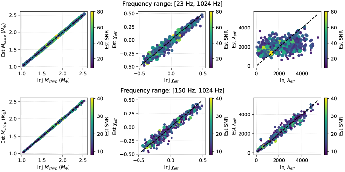
In this work, we show that in the full frequency band of the detectors, spins can interfere with the accurate measurement of the tidal deformability parameters. Thus, we focus on the late-inspiral part of the signals by starting the analyses at a higher frequency ($f\textsubscript{lower}\sim$ 150 Hz), using the data available just seconds before the merger. Using simulations, we show that this approach can efficiently provide accurate estimates of the effective tidal parameter, $\lambda\textsubscript{eff}$ in the presence of the component spins. Here we consider the component spins that are aligned to the orbital angular momentum of the binary system. Note that $\lambda\textsubscript{eff}$ is better estimated than the individual tidal deformability parameters in a similar sense that the mass-weighted effective spin parameter, $\chi\textsubscript{eff}$ is more accurately measured than the individual aligned-spins. These two quantities represent effects that are not explicitly correleated and can be independently calculated using

$$\chi\textsubscript{eff}=\frac{m_{1}\chi_{1z}+m_{2}\chi_{2z}}{m_{2}+m_{2}}\,,$$ (1)

$$\lambda\textsubscript{eff}=\frac{16}{13}\frac{m_{1}^{4}(m_{1}+12m_{2})\lambda_{1}+m_{2}^{4}(m_{2}+12m_{1})\lambda_{2}}{(m_{2}+m_{2})^{5}}$$ (2)

where $m_{i}$, $\chi_{i}$ and $\lambda_{i}$ represent the individual masses, the dimensionless spin parameters and the dimensionless tidal deformability parameters respectively.

There are several techniques to blend these effects together into waveform models. The classical approach using the post-Newtonian (PN) approximation is mostly valid in the low frequencies of the signal when the separation of the components is large . Using the effective-one-body (EOB) formalism, it is possible to include the tidal corrections till the initial contact of the two bodies (Nagar et al., 2018). In general, the coalescence of a neutron star merger becomes increasingly difficult to model as the components reach the merger, a regime where the numerical relativity (NR) informed approaches are expected to be more accurate (Damour & Nagar, 2010; Dietrich et al., 2019; Colleoni et al., 2023). It is also possible to incorporate the NR tidal corrections to precessing spin waveform models. However, parameter estimations using these waveform models have inferred only nominal spins for the GW events reported so far (Abbott et al., 2019; Dai et al., 2018; De et al., 2018; Abbott et al., 2018, 2020).

The work is organized as follows. In Section 2, we discuss an overview of the GW searches for BNS systems involving spin as well as the tidal effects. We use particle swarm optimization (PSO) for recovering signals from the data. PSO is a stochastic algorithm that iteratively optimizes a given fitness function in an arbitrary dimensional parameter space. We demonstrate a novel method to efficiently decouple the effective spin and the effective tidal deformability. We primarily investigate the match computed between the data and model waveforms starting at different low frequency cutoffs. The inner product between two vectors $a$ and $b$ is given by

$$\langle{a|b}\rangle=4\Re{\int_{f\textsubscript{lower}}^{f\textsubscript{upper}}\frac{\tilde{a}(f)\tilde{b}^{*}(f)}{S\textsubscript{n}(f)}}df\,.$$ (3)

Here $S\textsubscript{n}(f)$ represents the power spectral density (PSD) of the data which downweights the contribution of noise in the desired frequency domain $[f\textsubscript{lower},f\textsubscript{upper}]$. In Section 3, we report our observations for GW170817 using the new approach and discuss a prospective strategy for such analyses in the upcoming observing scenarios. We make a brief remark on the computational cost of the analyses conducted with the new approach.

2 METHODS

Figure 1: Recovery of the reweighted SNRs with various simulated searches for several BNS signals simulated using IMRPhenomXP_NRTidalv2. The searches are carried out with a 2 detector (HL) network and a time-coincidence test is used to arrive at the coincident detection statistic. Note that the quantity on the y-axis is the reweighted SNR for the coincident triggers which is computed with the standard $\chi\textsuperscript{2}$-veto (Allen, 2005). Since each search was carried out at the same template-sampling, we note that a search using templates with the tidal paremeters and large aligned-spin components is generally optimal.

Figure 2: Rates of background events compared for various searches obtained by running them on arbirary 4096 sec datasets from O3b. Background events are created by artificially time-sliding triggers from two or more detectors generated by the searches. The time slide duration is chosen to be larger than the maximum time taken by a GW signal to travel across detector, making the resulting events non-astrophysical. Searches identify astrophysical events by comparing their detection statistic against such background events from their local neighbourhood in time. The black dashed lines are for the searches on simulated Gaussian noise.

2.1 Searches with the tidal parameters

Gravitational wave searches constitute the first steps of astrophysical data processing whenever the analyzable data arrive from the observatories after calibration. The broad goal of the searches is to essentially identify events of astrophyical origin from the strain timeseries data to enable detailed follow-up investigations on them. The candidate events need to be consistent with several astrophysical assumptions such as that the triggers at different detectors caused by astrophysical events cannot be separated in time by more than the light’s travel time between the detectors. Triggers are computed from the matched-filter SNR timeseries, $\rho(t)$, realizing Eq. 3 with the strain data $h$ and a template waveform $q$

$$\rho^{2}(t;{\bm{\theta}})=4\Re{\int_{f\textsubscript{lower}}^{f\textsubscript{upper}}\frac{\tilde{h}(f)\tilde{q}^{*}(f;{\bm{\theta}})}{S\textsubscript{n}(f)}}e\textsuperscript{2{$\pi$}ift}df\,.$$ (4)

The data from the observatories are cross-correlated with banks of template waveforms that include various physical parameters ($\bm{\theta}$) describing the binaries. The number of the such parameters is often regarded as the search space dimensionality. Specific search configurations are adequately described in the literature (Usman et al., 2016; Adams et al., 2016; Messick et al., 2017; Venumadhav et al., 2019; Chu et al., 2022). Searches for binary neutron stars in the Advanced LIGO - Advanced Virgo era have generally included small aligned-spins in addition to the component masses for the templates (Aubin et al., 2021; Ewing et al., 2024; Canton et al., 2021). The first template bank search for neutron star mergers with the tidal parameters was only conducted recently by (Chia et al., 2023). However, their templates did not include any spin and resulted into no additional significant detection. Instead the search reported even smaller SNRs for some of the events already detected by aligned-spin searches. In general, including larger parts of the existing parameter space or extending the dimensionality of the existing parameter space is computationally challenging and can also result into higher levels of background events. We test the detection algorithm based on PSO to include the tidal parameters in the presence of aligned-spins. PSO allows us to explore a higher-dimensional search space without the need of designing and validating a template bank while requiring a relatively smaller number of template point realizations. The algorithm finally returns the optimal detection statistic along with a set of the point estimates for the source parameters in a frequenctist way (Pal & Nayak, 2023) . However, here we do not explicitly conduct a search targeting real events over the archived LIGO-Virgo-KAGRA (LVK) data and conclude based on simulations only. For this, we inject about 1000 simulated signals starting at 20 Hz into simulated data segments having O4 model noise PSDs. The component masses and the tidal parameters are randomly chosen from $[1M_{\odot},3M_{\odot}]$ and $[0,4000]$ respectively having a uniform distribution. These injections carry precessing spins with each spin component having a normal distribution around zero with the spin magnitudes restricted upto 0.95.

The signals are recovered with different combinations and/or ranges of template parameters using the PSO-based search algorithm. We use the TaylorF2 model to generate templates choosing from a subset of parameters given in Eq. 5. A combination includes at least the individual aligned-spins or the tidal parameters as the search parameters in addition to the component masses. The search space ranges are also allowed to vary for the aligned-spins. The maximum search dimensionality explored is 6 which includes both the aligned-spin and the tidal parameters.

$$\bm{\theta}=\{m_{1},m_{2},\chi_{1z},\chi_{2z},\lambda_{1},\lambda_{2}\}\,.$$ (5)

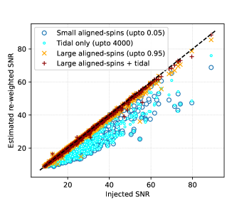
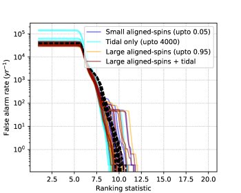
Within the PSO framework, the following two factors independently affect the recovery of the optimal match between the data and a template- (a) the waveform model, which ensures that the template is equipped with the physics to adequately model the incoming signal and (b) the template sampling, which ensures that a sufficient matched-filter computations are performed throughout the search space in order to locate the peak value of the match function. For computational efficiency, a faster waveform model is preferred. On the other hand, the sampling is preset in a way that just recovers signals at their optimal statistic as demonstrated in Fig. 2. In this work, we have tuned the search so that for a given stretch of data, around 25500 template points are computed. These many points in the search parameter space are used to generate the template waveforms which are then used in the matched-filtering of the data from each detector. The resulting triggers from the individual detectors are processed with several consistency tests to obtain the coincident events. The events are assigned a detection statistic from their reweighted SNRs and a false alarm rate based on time-slides (Usman et al., 2016). The methods adapted for the PSO algorithm are described in (Pal & Nayak, 2023).

A summary of the simulation results is the following. Between spins and tides, the former play the dominant role in obtaining the optimal detection statistic. We find that the templates used in searches should have at least large aligned-spins to recover sources that may have generic spins. On the other hand, the tidal parameters appears to have very small contribution to the build-up of the detection statistic. A search with templates having tidal parameters but no spin can lose a significant fraction of the retrievable statistic. We also exercise these searches on real datasets from O3b that do not contain any reported GW signal or known hardware injection (Abbott et al., 2021a). These datasets are 4096 seconds in duration and the searches use a similar setup as described earlier. We observe that all the template configurations respond to the noise events from the detector data in a similar fashion, resulting into equivalent rates of non-astrophysical background events, as summarized in Fig. 2. Thus we conclude that the search parameter space should include the tidal parameters in the presence of large generic aligned-spins to approach the optimal sensitivity towards the observable binary neutron stars.

Figure 3: The correlation between the errors in the point estimates for $\chi\textsubscript{eff}$ and $\lambda\textsubscript{eff}$ obtained from the six-dimensional PSO search including spins and tides at two different $f\textsubscript{lower}$’s. At the same detection criterion, a smaller fraction of the total injected signals are recovered at the same detection criterion while using a higher $f\textsubscript{lower}\sim$ 150 Hz as expected. However, the point estimates of $\lambda\textsubscript{eff}$ for the commonly found injections are generally more accurate than those for $f\textsubscript{lower}\sim$ 20 Hz.

Figure 4: Contours containing the top likelihood points in a grid of $\lambda\textsubscript{eff}$ vs $\chi\textsubscript{eff}$ as a function of the low frequency cut-off for the template waveforms. The component masses are fixed to the injected values of a typical BNS source located at 200 Mpc.

Figure 5: Visualization of the template signals in the time domain to used to decouple the spin and the tidal effects. A template with a smaller $f\textsubscript{lower}$ (in grey) is effective for capturing the spin effects, while a template with a larger $f\textsubscript{lower}$ (in blue) can handle the portion when the tidal interactions are prominent. The analyses with the later requires significantly small duration of strain data before the merger, and thus can be fast and reliable for the matter related effects.

2.2 Estimation of the effective tidal parameter

In this section, we discuss the effect of the measurement correlation between the effective spin and the effective tide using the likelihood function. The likelihood ($\mathcal{L}$) of a signal with the parameters $\bm{\theta}$ in the data $d$ assuming a Gaussian noise model is given as

$$\mathcal{L}=e^{-\langle{d-h(\bm{\theta})|d-h(\bm{\theta})}\rangle/2}\,,$$ (6)

where $\langle{a|b}\rangle$ represents the inner product of two vectors $a$ and $b$ defined in Eq. 3. The likelihood function is extensively used in the Bayesian approach to generate the posterior probability distributions of a desirable subset of the parameters. Several of these parameters can be degenerate with one another- the measurement of one can interfere with the measurement of another. The log-likelihood ratio (LLR) is often used to quantify a competing signal hypothesis against the noise hypothesis which simplifies to,

$$LLR=\langle{d|h(\bm{\theta})}\rangle-\frac{1}{2}\langle{h(\bm{\theta})|h(\bm{\theta})}\rangle\,.$$ (7)

To understand the measurement correlation between the effective spin $\chi\textsubscript{eff}$ and the effective tidal parameter $\lambda\textsubscript{eff}$, we sample the LLR as a function of $\lambda\textsubscript{eff}$ and $\chi\textsubscript{eff}$ for a random BNS injection while keeping other signal parameters fixed at their injected values. The injected signal is for a simulated source with component masses ($1.4M_{\odot},1.4M_{\odot}$) at 200 Mpc generated using the IMRPhenomD_NRTidal waveform model. The signal is projected onto a simulated HL detector network (O3). For sampling the likelihood (or the LLR), we choose moderate values of $\chi\textsubscript{i}$ upto $\pm 0.5$ and $\lambda\textsubscript{i}$ upto $4000$ to generate an equally spaced grid of points in the $\chi\textsubscript{eff}$-$\lambda\textsubscript{eff}$ plane. These points can be easily obtained by varying the values of $\chi\textsubscript{i}$ and $\lambda\textsubscript{i}$ which are preserved thoughout the simulation. Finally the LLR is computed at all the grid points and the contours containing the top likelihood points are plotted. The likelihood computations are repeated by changing the value of $f\textsubscript{lower}$, as shown in Fig. 4. We observe that the contours include a broad range of values for $\lambda\textsubscript{eff}$ when the waveforms are computed from a small $f\textsubscript{lower}\sim$ 23 Hz whereas it peaks sharply near the injected $\chi\textsubscript{eff}$ value (blue). This trend keeps reversing on increasing the $f\textsubscript{lower}$ with the likelihood function becoming more contrained towards $\lambda\textsubscript{eff}$ (pink), in spite of the fact that the likelihood value diminishes in this process due to the loss of the signal strength in the relevant frequency band.

Figure 6: Summary of the point estimates of the intrinsic parameters of multiple simulated BNS sources in zero noise recovered by the PSO search. The search parameters are ($m_{1},m_{2},\chi_{1z},\chi_{2z},\lambda_{1},\lambda_{2}$) whereas other remaining parameters were fixed at their injected values. The top and the bottom panels are for the two frequency ranges [23 Hz - 1024 Hz] and [150 Hz - 1024 Hz] analyzed with the configuration otherwise. From the rightmost plots, we note that the estimates for $\lambda\textsubscript{eff}$ can be obtained more accurately at the given sampling but at a much lower computational cost with $f\textsubscript{lower}\sim$ 150 Hz.

Figure 7: Multiple random injections recovered with single swarm in the simulated HL network using the PSO algorithm in the 150 Hz - 1024 Hz frequency range. We have chosen LLR to be the fitness function and show the SNR values corresponding to the peak LLR values obtained from PSO.

Figure 8: A GW170817-like injection recovered from simulated Gaussian noise using PSO. Each curve represents a swarm independently exploring the search parameter space as described in the text. The plot indicates that the algorithm picks up the optimal fitness value within 20 iterations while using $\sim$ 10000 particles per iteration. The injected fitness is computed at the injected signal parameters.

	Injection			Recovery
Parameter	Minimum	Maximum		Minimum	Maximum
Primary mass, $m_{1}$ $(M_{\odot})$	1	3		1	3
Secondary mass, $m_{2}$ $(M_{\odot})$	1	3		1	3
Primary z-spin, $\chi_{1z}$	-0.5	0.5		-0.5	0.5
Secondary z-spin, $\chi_{2z}$	-0.5	0.5		-0.5	0.5
Primary tidal deformability, $\lambda_{1}$	0	4000		0	4000
Secondary tidal deformability, $\lambda_{2}$	0	4000		0	4000
Coalescence time, $t_{c}$ (GPS seconds)	1100000000	1500000000		$t_{c}-0.01$	$t_{c}+0.01$
Distance, $D_{L}$ (Mpc)	50	60		$D_{L}-30$	$D_{L}+30$
Inclination, $\iota$ (rad)	0	$\pi$		$\iota-0.1$	$\iota+0.1$
Right ascension, $\alpha$ (rad)	0	$2\pi$		$\alpha-0.1$	$\alpha+0.1$
Declination, $\delta$ (rad)	$-\pi/2$	$\pi/2$		$\delta-0.05$	$\delta+0.05$
Coalescence phase, $\phi$ (rad)	0	$2\pi$		$0$	$2\pi$
Polarization, $\psi$ (rad)	0	$2\pi$		Marginalized
Table 1: Injection and estimation ranges of the signal parameters using the PSO algorithm as described in the text. The intrinsic parameters are searched over their respective possible domains while the extrinsic parameters are searched over a small window around their true values or can be marginalized over. The simulations and the results of this work are carried out with these settings unless stated otherwise.

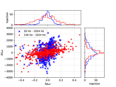
In the above simulation, we assumed the masses to be fixed at the injected values for computing the likelihood, however in real cases, the component masses are unknown and thus need to be estimated as free parameters. In fact in the most general case, all the signal parameters need to be treated as free parameters and be searched over their possible domains. However, in the following study we just free the component masses to explore the resulting six-dimensional space, since for the current scope, we are interested in obtaining intrinsic parameters accurately, specifically the tidal parameters, as summarized in Fig. 6. We keep other extrinsic parameters like the coalescence time, sky location, distance, etc. fixed at their injected values. In practice, this can also be tackled with a suitable marginalization scheme or by roughly treating some parameters as semi-free parameters that are available from external observations. For example, in the case of GW170817, we can combine the information from the EM observations and use the known sky position to sample over a smaller window for optimization. On the other hand, the coalescence time of the event can be sampled around the trigger time of the GW event which is a standard practice in GW parameter estimation. Since computing the likelihood function on such a high-dimensional space with a regular grid is computationally expensive and also not optimal, we use PSO with the LLR as the fitness function. The injection distribution of this simulation is similar to that mentioned in the previous section except that these injections are non-precessing with uniform aligned-spin components generated and recovered using the IMRPhenomD_NRTidal model.

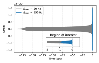
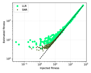
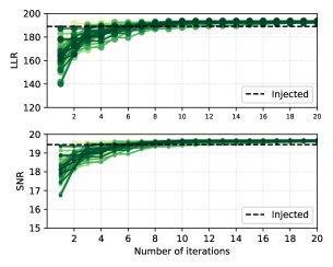
Fig. 7 shows the efficiency in recovering the LLR (or the SNR) as compared to the true LLR (or the true SNR) for multiple random injections. This is obtained by releasing the extrinsic parameters as semi-free parameters as shown in Table. 1. The PSO algorithm stochastically locates the optimal solution, realizing the maximum likelihood or match through a point estimate in the search parameter space. The parameter values of the optimally matching template are prone to statistical variations from several sources, for example from a random fluctuation due to a specific noise realization or the choice of the seed for initializing the algorithm. Note that with a higher $f\textsubscript{lower}$, the computational cost of the analysis becomes reasonably small mainly due to (a) the smaller duration of the data that is analyzed, $\sim 4$ seconds before the merger and (b) the faster generation of template waveforms due to the smaller number of inspiral cycles computed. We find that these analyses take seconds (or minutes) on multi-core (or single-core) machines. The reduced computational cost also makes it possible to conduct multiple rounds of the same analysis, each with a different seed to initialize the PSO algorithm. Thus, begining with a distinct seed, the algorithm chooses a distinct path, eventually converging on the contour of the optimal likelihood, which we call a multi-swarm exploration. This is demonstrated in Fig. 8 for a GW170817-like injection. We infer the source parameters from the resulting distribution of the point estimates thus obtained as described in the next section.

3 Observing scenarios

3.1 Current observations

Figure 9: Errors in the point estimates of $\lambda\textsubscript{eff}$ averaged over 10k simulated sources plotted as a function of the low frequency cutoff in O3-like sensitivity. At frequencies below 100 Hz, the measurement of $\chi\textsubscript{eff}$ overwhelms the measurement of $\lambda\textsubscript{eff}$ as indicated in Fig. 4. On the other hand, the fall in the signal strength beyond approximately 300 Hz, inhibits the possible improvement with a higher $f\textsubscript{lower}$. Two different waveform models are tested- TaylorF2 and IMRPhenomD_NRTidal. Note that the later is expected to give more reliable estimates with the new approach based on the late-inspiral.

Figure 10: Parameters reconstructed from the optimal template points reported by the multiple swarms that are used to independently explore the GW170817 event in the frequency range 150 Hz - 1024 Hz. Only the intrinsic parameters are shown. The extrinsic parameters like the sky location and the luminosity distance are sampled around the values reported from EM observations or are marginalized over as indicated in Table 1.

Figure 11: Uncertainties in the likelihood contours due to different noise realizations for a GW170817-like injection. Projected PSDs for the instruments are used to simulate the different observing scenarios. The colour shades represent the noise realization instances. We note that the variations could cause non-negligible differences in the final inferences at O4-like sensitivities but tend to stabilize in the upcoming observing scenarios.

Figure 12: Errors in the point estimates for 1k simulated sources with different PSDs in the frequency band 150 Hz - 1024 Hz (in yellow). The method provides unbiased estimates throughout various observing scenarios but in general, provides more accurate estimates as the sensitivies in the relevant frequency band gradually improve.

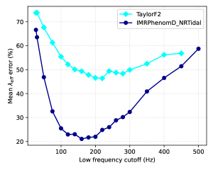
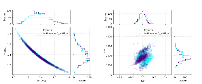
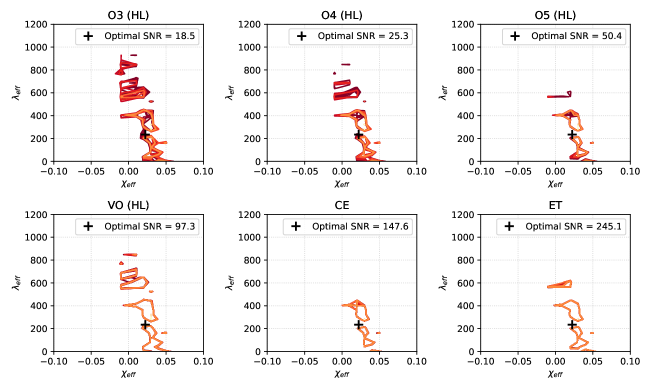
In the previous section, we discussed the PSO algorithm in the 6D intrinsic parameter space. Here we are interested in the BNS signals from the Advanced LIGO and the Advanced Virgo observing runs, whose extrinsic parameters like the sky location, the luminosity distance and the inclination angles are approximately known from observations. The BNS events reported so far are GW170817 and GW190425. The latter was observed only by the LIGO Livingston observatory and no electromagnetic counterpart could be observed. On the other hand, the former event was recored at both the LIGO Hanford and the LIGO Livingston observatories with a coincident network SNR $>$ 32 in the $\sim$ 23 Hz - 1024 Hz band, making it the loudest GW event till the end of O3. The HL coincident SNR of $\sim$ 16 in the $\sim$ 150 Hz - 1024 Hz band apparently makes it a suitable candidate for our analysis. A sub-threshold signal was also observed in Virgo improving the sky localization of the source. The sky location and the distance information for the source are also approximately known from other astronomical (EM) observations (Soares-Santos et al., 2017; Cantiello et al., 2018). We conduct the multi-swarm analyses with the GW data $\sim$ 4 seconds close to the merger time of the event with the goal of getting more insights on its tidal effects.

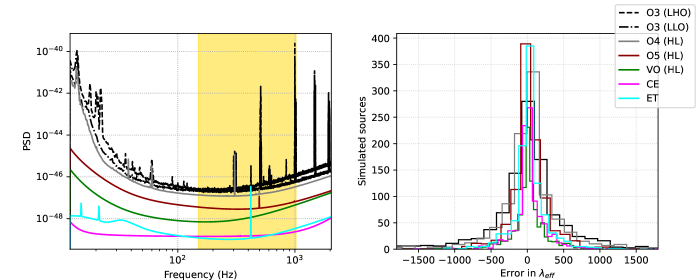
While we expect that the estimation of $M\textsubscript{chirp}$ and $\chi\textsubscript{eff}$ are more accurate in the full frequency range, this analyses still provides comparable estimates with the previously reported results. The component mass estimates are consistent with the $M\textsubscript{chirp}$-uncertainty contour, which we expect to be slightly broadened due to the smaller signal strength in the chosen analysis band, whereas the estimated $\chi\textsubscript{eff}$ is fairly consistent with a nominal value as shown in Fig. 10. As demonstrated in the earlier section, $\lambda\textsubscript{eff}$ which is expected to be better estimated with a higher $f\textsubscript{lower}$, is significantly different from that of the previously reported results (Abbott et al., 2019; Dai et al., 2018; Radice, 2019; De et al., 2018). However, note that such an estimate is prone to variations arising from the random noise fluctuations and the inference can be dependent on the specific noise realization of the instruments at the time of recording of the signal. The underlying variations are indicated for scenarios in O3 and beyond in Fig. 11. Thus, we cannot establish the true estimate for $\lambda\textsubscript{eff}$ with certainty based on the above observation, primarily due to the effect of the noise realization. Note that in the full Bayesian setting, a 90% credible region could exceedingly miss the true values at the current or past sensitivities as discussed in (Wade et al., 2013). Either multiple such observations are needed to reduce the effect of noise realizations from the detectors or exceptionally loud events can possibly inform us about the true tidal deformability parameters in the future. Thus, we do not explore further implications on the EoS of neutron stars based on the above inferences. However, we can conclude that a less stiff EoS may not be strictly ruled out based on the few observed neutron star binaries. This may be in contradiction to the general preference for a stiff EoS in the community.

3.2 Future observations

Figure 13: Simulation of NSBH systems differing in the BH mass with the masss of the NS is fixed at $1.4M_{\odot}$ for varying $f\textsubscript{lower}$. The contours represent top 97% values of the likelihood function computed in a similar fashion as in Fig. 4. We use the IMRPhenom_NSBH waveform model for generating the injection and the templates.

In the next generation of ground-based GW detectors, the rate of detections is likely to increase depending on the astrophysical abundancy of the sources and the factors like the sensitivity and the uptime of the instruments. The total SNR of the majority of the detectable events could be significantly large given the number of low-frequency inspiral cycles that the plausible $f\textsubscript{lower}$ would contain. Roughly, a signal from $1M_{\odot}-1M_{\odot}$ would last for more than 10,000 seconds in a detector’s sensitive frequency band starting at, say 5 Hz. Data analysis, including the standard Bayesian parameter estimation, of such long signals is a general challenge for GW astronomers. However, with the proposed sensitivities of the Cosmic Explorer (CE) and the Eintein Telescope (ET), a GW170817-like event could still register SNRs greater than 100, even with a higher $f\textsubscript{lower}$ as shown in Fig. 11. We find that in such scenarios , the effects of the random fluctuations from different noise realizations would be negligible and can thus, lead to reliable inferences from the estimated tidal parameters. For these future observations, the tidal properties can be efficiently extracted by exploring only the higher frequencies, despite the improvement in the low frequency sensitivities of the detectors like CE and ET. We expect the spin-tidal measurement correlation to become more pronounced for the full frequency band analyses with the improved low frequency sensitivities. Thus the method presented here can be promising, however, to include the related effects at further higher frequencies, a higher sampling rate would be considered (e.g. to increase $f\textsubscript{upper}$ from 1024 Hz to 2048 Hz, we just need to increase the sampling rate from 2048 Hz to 4096 Hz ). Note that the $M\textsubscript{chirp}$ information for low mass binaries is a fairly accurate byproduct of the detection algorithms. The technique proposed here could possibly lead to data products that provide valuable insights on the EM properties of the sources and can also be used to provide source classification in low-latencies.

4 Conclusions

This study shows that ignoring large generic aligned-spins in the presence/absence of tides in the detection stage leads to sub-optimal recovery of neutron star signals. However, the measurement of the effective spin parameter of the neutron star components can affect the measurement of the effective tidal parameter in the full frequency bandwith of the detectors. We have discussed a novel technique to extract the tidal information primarily from the late-inspiral part of neutron star mergers signals observable with the ground-based detectors. Though a restricted frequency band reduces the recovered SNR, we find the strategy effective in probing the tidal deformability effects in binary systems. We have also explored an empirical low frequency cutoff, $f\textsubscript{lower}$ for the signals that minimizes the errors in the point estimates of the effective tidal parameter, $\lambda\textsubscript{eff}$ using particle swarm optimization (PSO). We observed that a frequency band around 150 Hz - 1024 Hz efficiently provides more reliable estimates for a test population of simulated binary neutron stars than the full frequency band. We also found that this technique benifits from the numerical relativity (NR) informed waveform models which excel in modeling the near-coalescence regime. The study can be extended further to understand the correlation with/among other effects such as eccentricity and spin-precession.

For GW170817-like events, we conclude that with this method, the $\lambda\textsubscript{eff}$ estimates are expected to become free from uncertainties due to the detectors’ noise realizations in the future observing plans. The new approach could be especially effective in the upcoming observing scenarios when the duration of these signals would be longer and hence, computationally challenging with the improved/proposed low frequency sensitivities of the current and the upcoming ground-based detectors. Further investigations with the above strategy are desirable for binaries containing sub-solar mass objects or black holes accompanying the neutron stars.

In the case of neutron star-black hole (NSBH) systems, we observe that the tidal deformability of the NS tends to depend on the mass of its BH counterpart, as shown in Fig. 13. It is believed that the tidal deformability of a BH is zero which can be used as a test of the BH-nature of a component. However, the BH can cause measurable tidal deformability to the accompanying NS under some circumstances. As demonstrated in this work, the tidal component is almost uninforming at $f\textsubscript{lower}\sim 20$ Hz and starts constraining at a higher $f\textsubscript{lower}$. Nevertheless, we find that even at a higher $f\textsubscript{lower}$, the contours tend to be unconstrained for large mass ratios ($q$) systems, possibly indicating the absence of a measurable tidal deformability. Because a large mass BH would merge quickly with a typical NS, thus allowing almost no time to tidally deform and disrupt the NS. Generally, the tidal interactions can be expected when the BH mass is comparable to the NS mass, while also increasing the chances for an EM emission. We also encourage the readers to refer to an interesting discussion in the following review article (Chatziioannou, 2020).

5 Acknowledgments

This research has made use of data or software obtained from the Gravitational Wave Open Science Center (gwosc.org), a service of LIGO Laboratory, the LIGO Scientific Collaboration, the Virgo Collaboration, and KAGRA. LIGO Laboratory and Advanced LIGO are funded by the United States National Science Foundation (NSF) as well as the Science and Technology Facilities Council (STFC) of the United Kingdom, the Max-Planck-Society (MPS), and the State of Niedersachsen/Germany for support of the construction of Advanced LIGO and construction and operation of the GEO600 detector. Additional support for Advanced LIGO was provided by the Australian Research Council. Virgo is funded, through the European Gravitational Observatory (EGO), by the French Centre National de Recherche Scientifique (CNRS), the Italian Istituto Nazionale di Fisica Nucleare (INFN) and the Dutch Nikhef, with contributions by institutions from Belgium, Germany, Greece, Hungary, Ireland, Japan, Monaco, Poland, Portugal, Spain. KAGRA is supported by Ministry of Education, Culture, Sports, Science and Technology (MEXT), Japan Society for the Promotion of Science (JSPS) in Japan; National Research Foundation (NRF) and Ministry of Science and ICT (MSIT) in Korea; Academia Sinica (AS) and National Science and Technology Council (NSTC) in Taiwan.

This material is based upon work supported by NSF’s LIGO Laboratory which is a major facility fully funded by the National Science Foundation. The article has a LIGO Document number LIGO-P2400130. We have primarily used the PyCBC software in conducting various analyses in this work. We acknowledge the use of the Sarathi computing cluster at IUCAA for computational/numerical work. A significant part of the numerical work was also carried out at the Center of Excellence in Space Sciences, India (CESSI). CESSI is a multi-institutional Center of Excellence hosted by the Indian Institute of Science Education and Research (IISER) Kolkata and has been established through funding from the Ministry of Education, Government of India. SP wants to thank the financial support from the Council for Scientific and Industrial Research (CSIR), India through File No:09/921(0272)/2019-EMR-I.

References

- Abbott et al. (2020) Abbott, B. P., Abbott, R., Abbott, T. D., et al. 2020, The Astrophysical Journal Letters, 892, L3, doi: 10.3847/2041-8213/ab75f5
- Abbott et al. (2017a) Abbott, B. P., Abbott, R., Abbott, T., et al. 2017a, Physical review letters, 119, 161101, doi: 10.1103/PhysRevLett.119.161101
- Abbott et al. (2017b) Abbott, B. P., Abbott, R., Abbott, T. D., et al. 2017b, The Astrophysical Journal Letters, 848, L13, doi: 10.3847/2041-8213/aa920c
- Abbott et al. (2018) Abbott, B. P., Abbott, R., Abbott, T., et al. 2018, Physical review letters, 121, 161101
- Abbott et al. (2019) Abbott, B. P., Abbott, R., Abbott, T. D., et al. 2019, Phys. Rev. X, 9, 011001, doi: 10.1103/PhysRevX.9.011001
- Abbott et al. (2021a) Abbott, R., Abbott, T. D., Abraham, S., et al. 2021a, SoftwareX, 13, 100658, doi: https://doi.org/10.1016/j.softx.2021.100658
- Abbott et al. (2021b) —. 2021b, The Astrophysical Journal Letters, 915, L5, doi: 10.3847/2041-8213/ac082e
- Adams et al. (2016) Adams, T., Buskulic, D., Germain, V., et al. 2016, Classical and Quantum Gravity, 33, 175012, doi: 10.1088/0264-9381/33/17/175012
- Allen (2005) Allen, B. 2005, Physical Review D, 71, 062001, doi: 10.1103/PhysRevD.71.062001
- Aubin et al. (2021) Aubin, F., Brighenti, F., Chierici, R., et al. 2021, Classical and Quantum Gravity, 38, 095004, doi: 10.1088/1361-6382/abe913
- Cantiello et al. (2018) Cantiello, M., Jensen, J. B., Blakeslee, J. P., et al. 2018, The Astrophysical Journal Letters, 854, L31, doi: 10.3847/2041-8213/aaad64
- Canton et al. (2021) Canton, T. D., Nitz, A. H., Gadre, B., et al. 2021, The Astrophysical Journal, 923, 254, doi: 10.3847/1538-4357/ac2f9a
- Chatziioannou (2020) Chatziioannou, K. 2020, General Relativity and Gravitation, doi: 10.1007/s10714-020-02754-3
- Chia et al. (2023) Chia, H. S., Edwards, T. D., Wadekar, D., et al. 2023, arXiv preprint arXiv:2306.00050
- Chu et al. (2022) Chu, Q., Kovalam, M., Wen, L., et al. 2022, Physical Review D, 105, 024023, doi: 10.1103/PhysRevD.105.024023
- Colleoni et al. (2023) Colleoni, M., Vidal, F. A. R., Johnson-McDaniel, N. K., et al. 2023, arXiv preprint arXiv:2311.15978
- Dai et al. (2018) Dai, L., Venumadhav, T., & Zackay, B. 2018, arXiv preprint arXiv:1806.08793
- Damour & Nagar (2010) Damour, T., & Nagar, A. 2010, Phys. Rev. D, 81, 084016, doi: 10.1103/PhysRevD.81.084016
- Damour et al. (2012) Damour, T., Nagar, A., & Villain, L. 2012, Phys. Rev. D, 85, 123007, doi: 10.1103/PhysRevD.85.123007
- De et al. (2018) De, S., Finstad, D., Lattimer, J. M., et al. 2018, Phys. Rev. Lett., 121, 091102, doi: 10.1103/PhysRevLett.121.091102
- Dietrich et al. (2019) Dietrich, T., Khan, S., Dudi, R., et al. 2019, Phys. Rev. D, 99, 024029, doi: 10.1103/PhysRevD.99.024029
- Ewing et al. (2024) Ewing, B., Huxford, R., Singh, D., et al. 2024, Physical Review D, 109, 042008
- Kastaun & Ohme (2019) Kastaun, W., & Ohme, F. 2019, Phys. Rev. D, 100, 103023, doi: 10.1103/PhysRevD.100.103023
- LVK Collaboration (2018) LVK Collaboration. 2018, LVK Algorithm Library - LALSuite, Free software (GPL), doi: 10.7935/GT1W-FZ16
- Messick et al. (2017) Messick, C., Blackburn, K., Brady, P., et al. 2017, Physical Review D, 95, 042001, doi: 10.1103/PhysRevD.95.042001
- Nagar et al. (2018) Nagar, A., Bernuzzi, S., Del Pozzo, W., et al. 2018, Physical Review D, 98, 104052
- Pal & Nayak (2023) Pal, S., & Nayak, K. R. 2023, arXiv preprint arXiv:2307.03736
- Radice (2019) Radice, D. 2019, The European Physical Journal A, doi: 10.1140/epja/i2019-12716-4
- Romero-Shaw et al. (2020) Romero-Shaw, I. M., Talbot, C., Biscoveanu, S., et al. 2020, Monthly Notices of the Royal Astronomical Society, 499, 3295, doi: 10.1093/mnras/staa2850
- Soares-Santos et al. (2017) Soares-Santos, M., Holz, D. E., Annis, J., et al. 2017, The Astrophysical Journal Letters, 848, L16, doi: 10.3847/2041-8213/aa9059
- Usman et al. (2016) Usman, S. A., Nitz, A. H., Harry, I. W., et al. 2016, Classical and Quantum Gravity, 33, 215004, doi: 10.1088/0264-9381/33/21/215004
- Venumadhav et al. (2019) Venumadhav, T., Zackay, B., Roulet, J., Dai, L., & Zaldarriaga, M. 2019, Phys. Rev. D, 100, 023011, doi: 10.1103/PhysRevD.100.023011
- Wade et al. (2013) Wade, L., Creighton, J. D. E., Ochsner, E., et al. 2013, LIGO DCC. https://dcc.ligo.org/public/0109/G1301182/002/Tidal_Paper.pdf