A holographic bottom-up approach to baryons
Abstract
In this work, we discuss the description of neutral baryons with and using two bottom-up approaches: the deformed background and the static dilaton. In both models, we consider a non-linear Regge trajectory extension motivated by the strange nature that baryons have. We found that both models describe these systems with an RMS error smaller than 10 . We also perform a configurational entropy calculation in both models to discuss hadronic stability.
I Introduction
Describing baryons in the AdS/QCD bottom approach follows the same path as meson states. We start with an action for bulk fields dual to baryons at the conformal boundary. However, confinement is performed slightly differently from the meson scenario. Confinement is understood in these bottom-up scenarios as a localization process, where the non-normalizable bulk modes become normalizable by adding properly an energy scale. This energy scale will later fix the Regge slope. This localization mechanism can be done by two possible alternatives: cutting off or deforming the AdS geometry, i.e., breaking the conformal invariance in the bulk.
The cutoff of the space leads to the so-called hardwall Boschi-Filho and Braga (2004); Erlich et al. (2005); de Teramond and Brodsky (2005) and softwall models Karch et al. (2006). The former is achieved by placing a D-brane into the AdS space. The locus of the brane defines the energy scale as , where is the lightest hadron on the Regge trajectory. The mass spectrum usually behaves as , which is unexpected from light-unflavored hadron phenomenology. Quantum mechanically, this model behaves qualitatively like an infinite square well. The softwall model case includes a dilaton field that can be static or dynamically generated Batell and Gherghetta (2008), smoothly breaking conformal invariance. The net effect of this dilaton is the emergence of linear confinement Karch et al. (2006) when considering quadratic dilaton profiles, leading to Regge-like behavior , with defined as the excitation number, expected for unflavored light. Quantum mechanically speaking, these holographic potentials defined with quadratic dilatons behave as harmonic oscillators in the polar plane.
The softwall model proposal has proved to be successful in describing the spectroscopy of light-unflavored hadrons Ballon Bayona et al. (2008a); Vega et al. (2011); Branz et al. (2010); Afonin (2010); Colangelo et al. (2008, 2011); Ballon Bayona et al. (2008b); Gutsche et al. (2012); Li et al. (2013); Li and Huang (2013); Li et al. (2017); Vega and Martin Contreras (2020), form factors Abidin and Carlson (2008a, b, 2009) structure functions Watanabe and Suzuki (2014), deep inelastic scattering Ballon Bayona et al. (2008b); Braga and Vega (2012). It has been extended to the light-front case Brodsky and de Teramond (2008a); de Teramond and Brodsky (2009); Brodsky and de Teramond (2008b), where it has opened an active research area for wave functions Brodsky and de Teramond (2006); Vega et al. (2009), form factors Sufian (2017); Chakrabarti et al. (2020), and spectroscopy Ahmady et al. (2021).
However, despite all its success in the light sector, it could not properly describe heavy mesons since their Regge trajectories are not linear. From the Bethe-Salpeter perspective, by including the quark constituent mass linearity is lifted, i.e., , where depends on the constituent mass Chen (2018a, b, c). Along with this issue comes the mesonic decay constants issue. For bottom-up models, the decay constants do not match the phenomenological expected behavior; mesonic decay constants (in units of MeV) are expected to decrease with the excitation number. For hardwall, they increase, and for softwall, they are degenerate. Attempts to preserve quadratic behavior and obtain acceptable phenomenological decays have been made in the past Grigoryan et al. (2010); Braga et al. (2016). However, as pointed out in Ref. Martin Contreras and Vega (2020a), decay constants also depend on the low- behavior of the dilaton field. This situation is precisely the scenario proposed in Ref. Braga et al. (2017) for heavy vector quarkonia.
Regarding the heavy-spectroscopy issue, Ref. Martin Contreras and Vega (2020b) has extended the softwall model to include non-linear Regge trajectories by promoting the quadratic dilaton to be deformed by a parameter that accounts constituent mass effects. This proposal was also successful in describing non- states such as hadroquarkonium, hadronic molecules, or hybrid mesons, as in Ref. Martin Contreras and Vega (2023), where configurational entropy is used as a tool to test the feasibility of the proposed holographic structures.
Ref. Andreev (2006) originally proposed the deformation of the AdS space in the context of gauge/string duality applied to describe the OPE expansion for the two-point function. In this work, the author proves how quadratic deformations in the AdS5 sector lead to Regge-like behavior. This observation leads to Ref. Forkel et al. (2007), where the authors extended this idea to compute Regge trajectories for mesons and baryons. Later, the geometric deformation was used in Ref. Folco Capossoli et al. (2020a) to describe glueballs and light baryons. These works have in common that deformations in the AdS geometry induce locality by transforming bulk modes into normalizable ones, realizing confinement. This fact is translated into the emergence of confining terms in the holographic potential. In this sense, deformations and softwall models are equivalent. However, the analytical behavior of eigenmodes is completely different. In this framework, it has been possible to describe proton structure functions Folco Capossoli et al. (2020b), electromagnetic form factors for nucleons Contreras et al. (2021) and pions Martin Contreras et al. (2022a).
Another tool has gained importance with the holographic approaches developed to describe hadrons, the configurational entropy. The original proposal Gleiser and Stamatopoulos (2012a, b); Gleiser and Sowinski (2013) addresses the connection between the information and physical solutions for a given system. This idea is connected to how the energy is localized in such solutions. This localization of energy is related to the emergence of order structures. Thus, the configurational entropy (CE) can be understood as a entropic measure of how system constituents are organized in space. Holographically, CE has been extended in works as Braga and da Rocha (2017, 2018) to describe black hole stability in AdS and heavy quarkonia. In particular, the authors found the connection between decay constants and configurational entropy. When the former decreases with the excitation number, the latter increases. This observation can be considered an insight into hadronic stability via holographic tools. In this line of research, several works have enriched the literature, as indicated by Refs. da Rocha (2021); Barreto and da Rocha (2022); Martin Contreras et al. (2022b); Zhao and Hou (2023); Martin Contreras et al. (2023).
In this work, we will consider the approach to heavy baryons using the deformed dilaton proposal in both softwall and deformed geometry models. We will also consider configurational entropy as a tool to test hadronic stability in these models.
This work is organized as follows. In Section II, we summarize the bottom-up description of baryons. In Section III, we use geometric deformations and static dilaton in the non-linear Regge trajectory context to describe baryons. Section IV has a detailed calculation of the configurational entropy for these fermionic systems. And finally, in Section V, we present our conclusions.
II Holographic approach to baryons
Let us consider the AdS5 space defined by the Poincarè line element as
| (1) |
where the warp factor is defined as , with the radius of the AdS curvature. The function is the geometric deformation that, for the softwall model case, will be fixed as zero. We will use Latin indices for five-dimensional bulk objects and Greek indices for four-dimensional boundary objects.
Baryons, as it is standard in AdS/QCD, are described by bulk fermionic fields. However, it is not a straightforward task compared to mesons, where the effect of a dilaton field (static or dynamically generated) enters directly into the holographic potential due to the coupling of the dilaton field with bulk fields dual to mesons. In the case of baryons, the dilaton field is factorized out from the equation of motion. Thus, different mechanisms have to be considered to model these states. This situation is avoided when geometric deformations are considered since the confinement information is condensed in the warp factor. The main objection now arises because the background is flavor-dependent.
We will describe fermionic fields in AdS backgrounds with deformation and dilaton fields, following the prescription defined in Gutsche et al. (2012); Folco Capossoli et al. (2020a).
Let us focus on baryons with dilaton fields. Refs. Vega and Schmidt (2009); Gutsche et al. (2012) pointed out, the dilaton field can be introduced as an anomalous dimension that modifies the fermion bulk mass
| (2) |
This modification ensures that the bulk modes become normalizable when considering dilaton-based models.
II.1 Spin 1/2 baryons
For baryons, the bulk action is written in the standard Dirac form as follows:
| (3) |
with as the Dirac gamma matrices in curved space, is a constant fixing the units in the action, and covariant spin-connected derivative operator is defined as
| (4) |
where is the spin connection, is the flat gamma matrix commutator. The equations of motion for these fields read as follows.
| (5) | |||||
| (6) |
For AdS5, the frame field is , where Latin indices denote the flat frame indices. Thus, for the spin-affine connection, the non-zero components are
| (7) |
Therefore, the Dirac equation for the bulk spinor can be written as
| (8) |
A similar expression can be found for the adjoint bulk spinor . Next, we introduce the chiral components for the bulk spinors as
| (9) |
Using this definition and after transforming to the Fourier space, the Dirac equation is written as
| (10) |
| (11) |
In the last equation, we used the boundary Dirac equation in Fourier space to introduce the baryonic mass .
To decouple these equations, we take the second derivative, and after some algebra, we obtain the Sturm-Louville form of the Dirac equation:
| (12) |
At this step, confinement emerges from the holographic potential . This potential is defined using the Boguliobov transformation
| (13) |
we obtain the Schrodinger-like form of the bulk equations of motion:
| (14) |
with and for the potential has the following structure
| (15) |
The eigenvalues of this potential will correspond to the spin baryon masses at the boundary. A similar behavior is found for the adjoint spinor solutions. Both left and right solutions have the same eigenvalue mass . Thus, following Folco Capossoli et al. (2020a), we choose left movers to be dual to baryons at the boundary. The last ingredient we must fix is the bulk mass to define the baryonic identity. We will discuss this topic in the next section.
In the next sections, we will discuss applying the non-quadratic dilaton and the deformed geometry in this formalism.
II.2 Spin 3/2 baryons
Let us consider spin 3/2 baryons defined using a Rarita-Schwinger bulk field. The bulk action in this case is given by Gutsche et al. (2012)
| (16) |
where is a bulk vector spinor, and the covariant derivative is defined as
| (17) |
with is the Levi-Civita affine connection in AdS5, that has the non-zero components given by
| (18) | |||||
| (19) | |||||
| (20) |
From the action principle (16), we obtain the following bulk equations of motion
| (21) |
Let us consider the gauge fixing. Since no holographic information should be explicitly written at the boundary, i.e., no dependence on the holographic coordinate is expected, we impose
| (22) |
As a consequence, we will have the following set of transverse conditions:
| (23) | |||||
| (24) |
The condition (24) follows considering the product of the antisymmetric products of the Dirac matrices with the symmetric spinor tensor field, i.e.
| (25) |
which is equivalent to the Dirac equation. Using the first transverse condition will lead to the second one (24).
After the gauge fixing process, and using the expressions for the covariant derivative in AdS5, we write the equations of motion for the bulk vector spinor as
| (26) |
which is the equation for spin 1/2 bulk fermions. The main difference is the bulk mass since the operators that define spin 3/2 baryons have a different scaling dimension than the spin 1/2 ones.
Therefore, following the same procedure exposed for spin 1/2 bulk spinor, we obtain the Schrodinger-like equation of motion as
| (27) |
with the holographic potential defined as
| (28) |
As in the spin 1/2 case, we consider baryons defined by left vector spinors. In the next sections, we will solve the eigenvalue problem for the non-quadratic and deformed geometry models.
III AS/QCD applied to baryons
This section will apply the above-mentioned machinery to describe the baryons spectrum.
These baryons were initially observed in cosmic ray experiments during the 1950s and have since been extensively studied in particle accelerators. These states are compounded by a pair of light quarks with an quark. They play a crucial role in understanding the strong force that binds quarks and the composition of protons and neutrons within atomic nuclei.
In particular we will focus on the neutral baryons, with and . We summarize the experimental masses in Tables 1 and 2. Neutral baryons, aside from the , decay into neutral kaons mostly. For the baryon, the dominant decay is .
In previous studies (see Chen (2024) and references therein), it has been found that the Regge trajectory depends on the constituent mass of quarks. Thus, if a hadron contains an or a heavy quark, the linearity of the trajectory ceases. Motivated by this observation, we employ the non-quadratic softwall model Martin Contreras and Vega (2020b) to address the neutral spectroscopy.
In the standard AdS/CFT prescription, baryonic states, created by boundary operators like with , are dual to bulk normalizable fermionic modes that scale as . This matching is a consequence of the so-called field/operator duality. These bulk fields obey the dynamics governed by action densities such as (3) and (16). The information regarding the hadronic identity, i.e., the dimension of , is condensed in the fermionic bulk mass . In general, for a given hadron, we can write the conformal dimension as a combination of the contribution from constituent quarks (twist) and the total orbital angular momentum as
| (29) |
In the case of baryons, the expression above becomes handy to deal with high fermionic spin. Higher spin contributions can be written with . For with spin 1/2 and 3/2, their are 0 and 1, respectively.
Since a baryonic state has three quarks, each with a scaling dimension of , the constituent scaling dimension is . By substituting these data into Eq.(29), we can easily obtain the conformal dimensions and for the trajectories.
From the AdS/CFT dictionary, we find the following relationship for the fermion bulk mass and its baryon conformal dimension, given by:
| (30) |
Therefore, according to Eq. (29), for the baryons we obtain and for and respectively.
III.1 Non-quadratic deformed background
This model is a variation of the proposal presented in Folco Capossoli et al. (2020a), where quadratic deformations of the AdS warp factor, in Poincare coordinates, describe light hadrons. For strange baryons, we propose and fix the dilaton to be zero. Thus, for the warp factor in the AdS metric, we can write the following expression.
| (31) |
The effect of the geometric deformation is to place confinement. For fermions in the AdS space, bulk modes are unbounded. However, the deformation causes the emergence of bounded states dual to baryons at the conformal boundary. Since we choose , the bulk mass reduces to the standard value of given by Eq. (30).
After these definitions, we obtain the Schrödinger-like equation for both the right and left bulk fermions as:
| (32) |
where is the four-dimensional fermion mass.
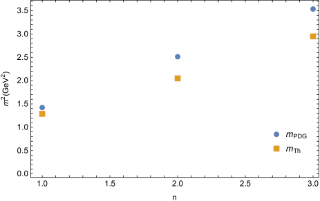
We fix the parameters in geometric deformation , given in Eq. (31) as MeV, MeV and for each baryonic trajectory. By entering these parameters in Eq.(32), we calculated a baryonic mass spectrum that is consistent with and trajectories, as indicated in Tables 1 and 2. The relative error is presented in the last columns of Tables 1 and 2. This error is calculated as follows
| (33) |
where depicts the deviations between the data and the model prediction .
| states | |||
| (MeV) | (MeV) | ||
| 1 | 1135.22 | 1192.60.02 | 4.81 |
| 2 | 1431.32 | 158520 | 9.70 |
| 3 | 1717.22 | 1820 to 1940 | 8.66 |
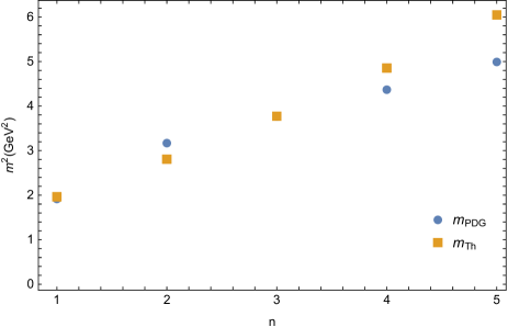
| states | |||
| (MeV) | (MeV) | ||
| 1 | 1401.37 | 1382.830.34 | 1.28 |
| 2 | 1675.77 | 1730 to 1830 | 5.86 |
| 3 | 1942.61 | 1920 to 1960 | 0.13 |
| 4 | 2203.36 | 2060 to 2120 | 5.42 |
| 5 | 2459.06 | 224027 | 10.07 |
We constructed Chew-Frautschi plots using data from Tables 1 and 2, which are presented in Figs.1 and 2. The figures show that the discrepancies between the calculated baryon masses and the experimentally measured mass data are below 10. Particularly noteworthy is the nearly identical masses for with , exhibiting an error of , while for with , the error is a strikingly low 0.13.
Additionally, we calculate the overall RMS error using the following definition:
| (34) |
where and are the number of measurements and parameters, respectively. In this case, we obtain the values of the parameters and for the and trajectories separately by fitting and assigning a common value for both trajectories. This choice comes from the Bethe-Salpeter analysis of Regge-trajectories Chen (2018a), where the constituent quark mass influences the linearity of the trajectory. Since both trajectories have the same quark content, it is natural to consider the same for them. From Eq.(34), we find that for trajectories using the deformed background.
III.2 Non-quadratic dilaton
This proposal is an extension of the non-quadratic dilaton idea developed for isovector mesons and non- states Martin Contreras and Vega (2020b, 2023). In the case of fermionic bulk fields, the dilaton field factors out from the equations of motion. However, confinement is addressed by inserting the dilaton an anomalous dimension, as we explain in section II.
In this prescription, we will set , and then the warp factor and the dilaton field can be written as
| (35) | |||||
| (36) |
Then, using Eq.(2), we obtain a Schrödinger-like equation:
| (37) |
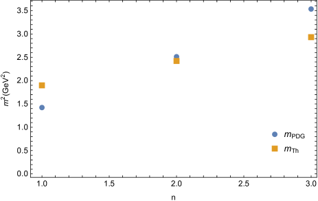
Notice that the bulk mass used here remains the same as in the deformed case. We set and , and substitute them into Eq.(37). The resulting data is displayed in Tables 3 and 4.
| states | |||
| (MeV) | (MeV) | ||
| 1 | 1377.51 | 1192.60.02 | 15.50 |
| 2 | 1555.77 | 158520 | 1.84 |
| 3 | 1712.28 | 1820 to 1940 | 8.92 |
| states | |||
| (MeV) | (MeV) | ||
| 1 | 1571.94 | 1382.830.34 | 13.60 |
| 2 | 1726.75 | 1730 to 1830 | 3.00 |
| 3 | 1866.39 | 1920 to 1960 | 3.79 |
| 4 | 1994.45 | 2060 to 2120 | 4.57 |
| 5 | 2113.28 | 224027 | 5.40 |
We have generated the Chew-Frautschi plot based on the data presented in Tables 3 and 4. The non-quadratic dilaton accurately matches the high excited states: the relative errors are below . However, the ground state is not well-fitted. It is unsurprising since the ground state strongly depends on the dilaton slope .
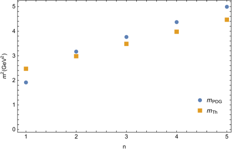
Lastly, we computed the total RMS error, and it is important to mention that we employed identical parameters for with different spins. Therefore, is involved in this calculation. From Eq.(34), we find for the family.
IV Configurational Entropy
IV.1 Configurational entropy and hadronic stability
The inspiration behind Configuration Entropy Gleiser and Stamatopoulos (2012a, b); Gleiser and Sowinski (2013) comes from Shannon’s information entropy Shannon (1948), a measure that quantifies the amount of information in a message Braga and Junqueira (2021). For a variable that can take discrete possible values, with probabilities given by , it is defined by
| (38) |
In the original formulation within information theory, configurational entropy (CE) can be understood as a measure of the information required to describe localized functions or sets of solution parameters. Generally, dynamical solutions emerge from optimizing an action, and configurational entropy measures the information available in these solutions. The relationship between configurational entropy and complexity is associated with stability. As configurational entropy characterizes the complexity of a given physical system, states with higher configurational entropy require more energy for their occurrence in nature compared to states with lower configurational entropy. Higher energy levels also imply more modes that conform to such physical states, indicating that configurational entropy increases with higher coarseness. Hence, configurational entropy can also be perceived as a measure of stability. Remember that configurational entropy reflects the relative ordering in field configuration space, illustrating the relationship between energy and coarseness. With an increase in constituents, there is a corresponding increase in energy and relative configurational entropy. Additionally, investigations on active matter systems demonstrate that the final state of a many-particle system minimizes configurational entropy when it reaches equilibrium.
Configuration Entropy is commonly used to describe the variety of particle spatial arrangements within a system at the microscopic scale. Its calculation involves determining the quantity and distribution of distinct microscopic states throughout the system. Specifically, CE measures the complexity and diversity within a system, reflecting the uncertainty associated with particle arrangements at the microscopic level. When computing the configurational entropy for the family, from a bottom-up perspective, we connect bulk localization of the dual fermionic modes with the stability at the boundary. This fact is connected with the observation that heavier states should decay faster than light ones. Thus, we expect that the CE decreases with the excitation level .
Thus, we can say that holographic CE indirectly measures the diversity and complexity of constituent spatial arrangements in the baryon family. A high configurational entropy in the system implies that the microscopic particle arrangement exhibits a high degree of randomness and disorder, potentially making the system more susceptible to decay or fragmentation, thus reducing its stability. In contrast, a low configurational entropy suggests a more compact and orderly microscopic particle arrangement, often indicative of a more stable system.
In recent years, numerous studies have focused on configurational entropy, including investigations into compact objects Gleiser and Jiang (2015) and holographic AdS/QCD models Bernardini and da Rocha (2016); Bernardini et al. (2017); Braga and da Rocha (2017, 2018); Braga et al. (2018); Bernardini and Da Rocha (2018); Ferreira and Da Rocha (2019); Martin Contreras et al. (2023), among other diverse systems. These studies, approached from various angles, consistently demonstrate a parallel relationship between changes in configurational entropy and stability. In this paper, we perform holographic calculations of the configurational entropy for baryons using different holographic models discussed in the previous section.
To do so, we compute the differential configurational entropy (DCE) for a given physical system by performing the following calculations for each model: Firstly, we obtain the localized solutions to the equations of motion. Then, we evaluate the on-shell energy density. Next, we transform the on-shell energy density into momentum space. Finally, we calculate the modal fraction and evaluate the DCE integral based on the results.
IV.2 Configurational entropy for baryons
The key ingredient for DCE comes from the on-shell energy-momentum tensor for the bulk fields. Since the AdS frame is static to these fields, it is possible to use the dynamical On-shell energy tensor is defined as
| (39) |
For the DCE, it is enough to consider this definition since gravity has not been affected by the fermionic fields. However, the variations must be done using the frame fields instead of the metric tensor. Thus, we will follow the prescription in Ref. Shapiro (2022). Therefore, from the action (3) we obtain for spin
| (40) |
and for spin , from action (16), we have:
| (41) |
The energy density in both cases is extracted from the component. For the spin field, after Fourier transform, we find
| (42) |
where is a polarization factor. The energy density for the spin field is
| (43) |
where and are polarization factors that appear from the contraction of the indices. For simplicity, we will choice . Then, we perform a Fourier transform on the energy density and express it as
| (44) |
The modal fraction, which describes how localized the information is in a given mode, is defined as
| (45) |
For the continuous variables case, we use the differential configurational entropy (DCE) defined as
| (46) |
where , and is the maximum value assumed by .
Recall that has information on how energy is localized in the bulk. Thus, it indirectly measures how normalizable modes are well localized in the AdS space. In hadronic terms, this localization measure is also a signal of confinement since a bounded state should be localized. Therefore, DCE becomes a clear test for holographic models mimicking hadrons.
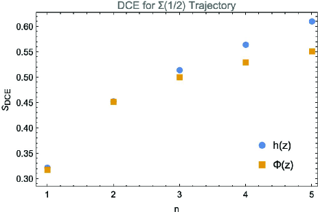
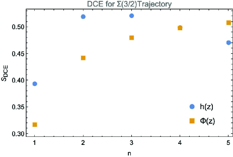
We calculated the differential configurational entropy (DCE) for the and trajectories using both bottom/up approaches. We summarize our findings in Figs.5 and 6.
As we expected from the localization and stability hypothesis, Fig. 5 shows that as increases, increases for the trajectory in both models. However, for the trajectory, the DCE only grows with for the non-quadratic dilaton approach. The deformed background approach increases only for the first excited state. Higher excitations have decreased the DCE. Assuming the DCE-stability hypothesis, these higher states become more stable. This conclusion is not possible from the hadronic phenomenology. Thus, deformed background approach is not good for describing these states.
V Conclusions
In this study, we developed two models: the non-quadratic deformed background with the warp factor set as . For the second model, we assume a non-quadratic dilaton . Using standard bottom-up techniques, we tested these models as alternatives to describe baryon spectroscopy. Each model has two parameters associated with the Regge slope and the linearity deviation. In both cases, experimental data was properly fitted, having RMS errors smaller than 10 . The next stage in choosing a good model is the DCE analysis.
Regarding the mass spectrum, we observed that ground states are not well-fitted in both models. In other bottom-up models, ground state mass sets the Regge slope. However, in this non-quadratic scenario, the slope and the deformation are fitted by regression over the entire trajectory. Ground states are strongly attached to the behavior of the one-gluon exchange term in hadronic potentials. These terms come from the perturbative analysis, which is not captured in the dilaton or deformations. Recall that this bottom-up confinement tries to mimic the confinement part in the Cornell-like potentials that control the higher excitations. Further improvements in the determination of the intercept (leading to a better ground state mass) are required. For further details, see Afonin and Solomko (2022) for an interesting discussion and review of how hadronic spectroscopy can be captured in bottom-up models.
Configurational entropy measures how well localized a mode is in the solution space. Thus, it could have information about confinement by considering that the emergence of bounded colorless states is a consequence of color confinement. Thus, DCE can be used to address whether or not a given holographic approach is suitable to describe hadrons from the stability point of view. However, DCE is not the only test we have. Thermal analysis Martin Contreras et al. (2022a) of the two-point spectral function also discusses stability.
For the models discussed here, we observed that the deformed background seems inconsistent with the hypothesis of stability/DCE, at least for the trajectory. As a hypothesis, if we analyze the behavior of the Schrödinger modes in the deformed background, we see that they are highly suppressed in the bulk due to the structure of the holographic potential, i.e., the exponential factor in Eqn. (15), the modes are spatially confined. For excited modes, they oscillate in small bulk regions. Since these solutions do not tend to smear out into the bulk, the DCE does not decrease. This hypothesis has to the tested with other similar geometric approaches.
From its original motivation, differential configurational entropy describes how constituents are distributed among different states or configurations in a given system. It allows us to quantify the degree of disorder or randomness of those constituent arrangements, providing insights into the probabilities of various particle configurations. Thus, DCE is related to how constituents interact with each other. This fact allows DCE to be considered a probe to test how confinement is realized in holographic models. However, there is still plenty of room to discuss the nature of the arrangements of constituents inside hadrons since how we model these systems in such holographic models has to be improved.
A higher differential configurational entropy indicates more possible particle arrangements, implying greater disorder or freedom of movement. On the other hand, a lower differential configurational entropy suggests a more ordered particle arrangement or more significant constraints on the configuration. The calculation results for the two models are shown in Figs. 5 and 6. From the figures, we can observe that the data overall increases with the increase in mass, and the values of configurational entropy also increase. By comparing the results of the two models, it is found that the model incorporating the dilaton field obtains lower configurational entropy in the calculation of and .
The relationship between configurational entropy and the mass spectrum of baryons is highly significant. Configurational entropy is an indirect measure of the intricacy of the structure in baryons. Meanwhile, the mass spectrum characterizes the distribution of masses corresponding to different energy levels and combinations of constituent particles within baryons. Higher configurational entropy in baryons signifies a broader range of arrangements and degrees of freedom. This observation can also be interpreted in terms of transition probabilities. Higher DCE is connected with smaller decay widths. Thus, the smallest DCE is expected to belong to the ground state with the highest decay width. We will explore this idea in further investigations.
Acknowledgements.
M. A. Martin Contreras wants to acknowledge the financial support provided by the National Natural Science Foundation of China (NSFC) under grant No 12350410371. X. Chen wants to acknowledge the financial support provided by Research Foundation of Education Bureau of Hunan Province, China (Grant No. 21B0402) and the Natural Science Foundation of Hunan Province of China under Grant No.2022JJ40344.References
- Boschi-Filho and Braga (2004) H. Boschi-Filho and N. R. F. Braga, Eur. Phys. J. C 32, 529 (2004), arXiv:hep-th/0209080 .
- Erlich et al. (2005) J. Erlich, E. Katz, D. T. Son, and M. A. Stephanov, Phys. Rev. Lett. 95, 261602 (2005), arXiv:hep-ph/0501128 .
- de Teramond and Brodsky (2005) G. F. de Teramond and S. J. Brodsky, Phys. Rev. Lett. 94, 201601 (2005), arXiv:hep-th/0501022 .
- Karch et al. (2006) A. Karch, E. Katz, D. T. Son, and M. A. Stephanov, Phys. Rev. D 74, 015005 (2006), arXiv:hep-ph/0602229 .
- Batell and Gherghetta (2008) B. Batell and T. Gherghetta, Phys. Rev. D 78, 026002 (2008), arXiv:0801.4383 [hep-ph] .
- Ballon Bayona et al. (2008a) C. A. Ballon Bayona, H. Boschi-Filho, N. R. F. Braga, and L. A. Pando Zayas, Phys. Rev. D 77, 046002 (2008a), arXiv:0705.1529 [hep-th] .
- Vega et al. (2011) A. Vega, I. Schmidt, T. Gutsche, and V. E. Lyubovitskij, Phys. Rev. D 83, 036001 (2011), arXiv:1010.2815 [hep-ph] .
- Branz et al. (2010) T. Branz, T. Gutsche, V. E. Lyubovitskij, I. Schmidt, and A. Vega, Phys. Rev. D 82, 074022 (2010), arXiv:1008.0268 [hep-ph] .
- Afonin (2010) S. S. Afonin, Int. J. Mod. Phys. A 25, 5683 (2010), arXiv:1001.3105 [hep-ph] .
- Colangelo et al. (2008) P. Colangelo, F. De Fazio, F. Giannuzzi, F. Jugeau, and S. Nicotri, Phys. Rev. D 78, 055009 (2008), arXiv:0807.1054 [hep-ph] .
- Colangelo et al. (2011) P. Colangelo, F. Giannuzzi, and S. Nicotri, Phys. Rev. D 83, 035015 (2011), arXiv:1008.3116 [hep-ph] .
- Ballon Bayona et al. (2008b) C. A. Ballon Bayona, H. Boschi-Filho, and N. R. F. Braga, JHEP 03, 064 (2008b), arXiv:0711.0221 [hep-th] .
- Gutsche et al. (2012) T. Gutsche, V. E. Lyubovitskij, I. Schmidt, and A. Vega, Phys. Rev. D 85, 076003 (2012), arXiv:1108.0346 [hep-ph] .
- Li et al. (2013) D. Li, M. Huang, and Q.-S. Yan, Eur. Phys. J. C 73, 2615 (2013), arXiv:1206.2824 [hep-th] .
- Li and Huang (2013) D. Li and M. Huang, JHEP 11, 088 (2013), arXiv:1303.6929 [hep-ph] .
- Li et al. (2017) D. Li, M. Huang, Y. Yang, and P.-H. Yuan, JHEP 02, 030 (2017), arXiv:1610.04618 [hep-th] .
- Vega and Martin Contreras (2020) A. Vega and M. A. Martin Contreras, Phys. Rev. D 102, 036017 (2020), arXiv:2005.04501 [hep-ph] .
- Abidin and Carlson (2008a) Z. Abidin and C. E. Carlson, Phys. Rev. D 77, 095007 (2008a), arXiv:0801.3839 [hep-ph] .
- Abidin and Carlson (2008b) Z. Abidin and C. E. Carlson, Phys. Rev. D 77, 115021 (2008b), arXiv:0804.0214 [hep-ph] .
- Abidin and Carlson (2009) Z. Abidin and C. E. Carlson, Phys. Rev. D 79, 115003 (2009), arXiv:0903.4818 [hep-ph] .
- Watanabe and Suzuki (2014) A. Watanabe and K. Suzuki, Phys. Rev. D 89, 115015 (2014), arXiv:1312.7114 [hep-ph] .
- Braga and Vega (2012) N. R. F. Braga and A. Vega, Eur. Phys. J. C 72, 2236 (2012), arXiv:1110.2548 [hep-ph] .
- Brodsky and de Teramond (2008a) S. J. Brodsky and G. F. de Teramond, Phys. Rev. D 77, 056007 (2008a), arXiv:0707.3859 [hep-ph] .
- de Teramond and Brodsky (2009) G. F. de Teramond and S. J. Brodsky, Phys. Rev. Lett. 102, 081601 (2009), arXiv:0809.4899 [hep-ph] .
- Brodsky and de Teramond (2008b) S. J. Brodsky and G. F. de Teramond, Phys. Rev. D 78, 025032 (2008b), arXiv:0804.0452 [hep-ph] .
- Brodsky and de Teramond (2006) S. J. Brodsky and G. F. de Teramond, Phys. Rev. Lett. 96, 201601 (2006), arXiv:hep-ph/0602252 .
- Vega et al. (2009) A. Vega, I. Schmidt, T. Branz, T. Gutsche, and V. E. Lyubovitskij, Phys. Rev. D 80, 055014 (2009), arXiv:0906.1220 [hep-ph] .
- Sufian (2017) R. S. Sufian, Phys. Rev. D 96, 093007 (2017), arXiv:1611.07031 [hep-ph] .
- Chakrabarti et al. (2020) D. Chakrabarti, C. Mondal, A. Mukherjee, S. Nair, and X. Zhao, Phys. Rev. D 102, 113011 (2020), arXiv:2010.04215 [hep-ph] .
- Ahmady et al. (2021) M. Ahmady, S. Kaur, S. L. MacKay, C. Mondal, and R. Sandapen, Phys. Rev. D 104, 074013 (2021), arXiv:2108.03482 [hep-ph] .
- Chen (2018a) J.-K. Chen, Phys. Lett. B 786, 477 (2018a), arXiv:1807.11003 [hep-ph] .
- Chen (2018b) J.-K. Chen, Eur. Phys. J. C 78, 235 (2018b).
- Chen (2018c) J.-K. Chen, Eur. Phys. J. C 78, 648 (2018c).
- Grigoryan et al. (2010) H. R. Grigoryan, P. M. Hohler, and M. A. Stephanov, Phys. Rev. D 82, 026005 (2010), arXiv:1003.1138 [hep-ph] .
- Braga et al. (2016) N. R. F. Braga, M. A. Martin Contreras, and S. Diles, Phys. Lett. B 763, 203 (2016), arXiv:1507.04708 [hep-th] .
- Martin Contreras and Vega (2020a) M. A. Martin Contreras and A. Vega, Phys. Rev. D 101, 046009 (2020a), arXiv:1910.10922 [hep-th] .
- Braga et al. (2017) N. R. F. Braga, L. F. Ferreira, and A. Vega, Phys. Lett. B 774, 476 (2017), arXiv:1709.05326 [hep-ph] .
- Martin Contreras and Vega (2020b) M. A. Martin Contreras and A. Vega, Phys. Rev. D 102, 046007 (2020b), arXiv:2004.10286 [hep-ph] .
- Martin Contreras and Vega (2023) M. A. Martin Contreras and A. Vega, Phys. Rev. D 108, 126024 (2023), arXiv:2309.02905 [hep-ph] .
- Andreev (2006) O. Andreev, Phys. Rev. D 73, 107901 (2006), arXiv:hep-th/0603170 .
- Forkel et al. (2007) H. Forkel, M. Beyer, and T. Frederico, JHEP 07, 077 (2007), arXiv:0705.1857 [hep-ph] .
- Folco Capossoli et al. (2020a) E. Folco Capossoli, M. A. Martín Contreras, D. Li, A. Vega, and H. Boschi-Filho, Chin. Phys. C 44, 064104 (2020a), arXiv:1903.06269 [hep-ph] .
- Folco Capossoli et al. (2020b) E. Folco Capossoli, M. A. Martín Contreras, D. Li, A. Vega, and H. Boschi-Filho, Phys. Rev. D 102, 086004 (2020b), arXiv:2007.09283 [hep-ph] .
- Contreras et al. (2021) M. A. M. Contreras, E. F. Capossoli, D. Li, A. Vega, and H. Boschi-Filho, Phys. Lett. B 822, 136638 (2021), arXiv:2108.05427 [hep-ph] .
- Martin Contreras et al. (2022a) M. A. Martin Contreras, E. Folco Capossoli, D. Li, A. Vega, and H. Boschi-Filho, Nucl. Phys. B 977, 115726 (2022a), arXiv:2104.04640 [hep-ph] .
- Gleiser and Stamatopoulos (2012a) M. Gleiser and N. Stamatopoulos, Phys. Lett. B 713, 304 (2012a), arXiv:1111.5597 [hep-th] .
- Gleiser and Stamatopoulos (2012b) M. Gleiser and N. Stamatopoulos, Phys. Rev. D 86, 045004 (2012b), arXiv:1205.3061 [hep-th] .
- Gleiser and Sowinski (2013) M. Gleiser and D. Sowinski, Phys. Lett. B 727, 272 (2013), arXiv:1307.0530 [hep-th] .
- Braga and da Rocha (2017) N. R. F. Braga and R. da Rocha, Phys. Lett. B 767, 386 (2017), arXiv:1612.03289 [hep-th] .
- Braga and da Rocha (2018) N. R. F. Braga and R. a. da Rocha, Phys. Lett. B 776, 78 (2018), arXiv:1710.07383 [hep-th] .
- da Rocha (2021) R. da Rocha, Phys. Rev. D 103, 106027 (2021), arXiv:2103.03924 [hep-ph] .
- Barreto and da Rocha (2022) W. Barreto and R. da Rocha, Phys. Rev. D 105, 064049 (2022), arXiv:2201.08324 [hep-th] .
- Martin Contreras et al. (2022b) M. A. Martin Contreras, A. Vega, and S. Diles, Phys. Lett. B 835, 137551 (2022b), arXiv:2206.01834 [hep-ph] .
- Zhao and Hou (2023) Y.-Q. Zhao and D. Hou, Phys. Lett. B 847, 138271 (2023), arXiv:2305.07087 [hep-ph] .
- Martin Contreras et al. (2023) M. A. Martin Contreras, A. Vega, and S. Diles, (2023), arXiv:2308.16007 [hep-ph] .
- Vega and Schmidt (2009) A. Vega and I. Schmidt, Phys. Rev. D 79, 055003 (2009), arXiv:0811.4638 [hep-ph] .
- Chen (2024) J.-K. Chen, Eur. Phys. J. C 84, 356 (2024), arXiv:2302.06794 [hep-ph] .
- Workman et al. (2022) R. L. Workman et al. (Particle Data Group), PTEP 2022, 083C01 (2022).
- Shannon (1948) C. E. Shannon, The Bell System Technical Journal 27, 379 (1948).
- Braga and Junqueira (2021) N. R. F. Braga and O. C. Junqueira, Phys. Lett. B 814, 136082 (2021), arXiv:2010.00714 [hep-th] .
- Gleiser and Jiang (2015) M. Gleiser and N. Jiang, Phys. Rev. D 92, 044046 (2015), arXiv:1506.05722 [gr-qc] .
- Bernardini and da Rocha (2016) A. E. Bernardini and R. da Rocha, Phys. Lett. B 762, 107 (2016), arXiv:1605.00294 [hep-th] .
- Bernardini et al. (2017) A. E. Bernardini, N. R. F. Braga, and R. da Rocha, Phys. Lett. B 765, 81 (2017), arXiv:1609.01258 [hep-th] .
- Braga et al. (2018) N. R. F. Braga, L. F. Ferreira, and R. a. Da Rocha, Phys. Lett. B 787, 16 (2018), arXiv:1808.10499 [hep-ph] .
- Bernardini and Da Rocha (2018) A. E. Bernardini and R. Da Rocha, Phys. Rev. D 98, 126011 (2018), arXiv:1809.10055 [hep-th] .
- Ferreira and Da Rocha (2019) L. F. Ferreira and R. Da Rocha, Phys. Rev. D 99, 086001 (2019), arXiv:1902.04534 [hep-th] .
- Shapiro (2022) I. L. Shapiro, Universe 8, 586 (2022), arXiv:1611.02263 [gr-qc] .
- Afonin and Solomko (2022) S. S. Afonin and T. D. Solomko, Eur. Phys. J. C 82, 195 (2022), arXiv:2106.01846 [hep-th] .