A general polarimetric model for transiting and non-transiting ringed exoplanets

Abstract

Context. The detection and characterization of exorings, i.e. rings around exoplanets, will be the next breakthrough in exoplanetary science. It will help us to better understand the origin and evolution of planetary rings in the Solar System and beyond. Exorings are still elusive, and new and clever methods for identifying them need to be developed and tested.

Aims. Polarimetry of the reflected light signals of exoplanets appears to be a promising tool to identify the tell-tale signatures of exorings. We explore the potential of polarimetry as a tool for detecting and characterizing exorings.

Methods. For that purpose, we have improved the general, publicly available photometric code Pryngles by adding the results of radiative transfer calculations with an adding-doubling algorithm that fully includes polarization; the improved package also allows for including the scattering by irregularly shaped dusty ring particles. With this improved code, we compute the total and polarized fluxes, and the degree of polarization of model gas giant planets with or without rings, along their orbits, for various key model parameters, such as the orbit inclination, ring size and orientation, ring particle albedo and optical thickness. We demonstrate the versatility of our code by predicting the total and polarized fluxes of the “puffed-up” planet HIP 41378 f assuming this planet has an opaque dusty ring.

Results. Spatially unresolved dusty rings can significantly modify the flux and polarization signals of the light that is reflected by a gas giant exoplanet along its orbit. Rings are expected to have a low polarization signal and will generally decrease the degree of polarization along the orbit of a planet-ring system as a whole as the ring casts a shadow on the planet and/or blocks part of the light the planet reflects. During ring-plane crossings, when the thin ring is illuminated edge-on, a ringed exoplanet’s flux and degree of polarization are close to those of a ring-less planet, and ring-plane crossing geometries generally appear as sharp changes in the flux and polarization curves. Ringed planets in edge-on orbits tend to be difficult to distinguish from ring-less planets in reflected flux and degree of polarization. A larger ring optical thickness, particle albedo, and/or ring width usually yields stronger ring characteristics in the phase functions. We also show that if HIP 41378 f is indeed surrounded by a ring, its reflected flux (compared to the star) will be of the order of $10^{-9}$, while the ring would decrease the degree of polarization in a detectable way.

Conclusions. The improved version of the photometric code Pryngles that we present here shows that dusty rings may produce distinct polarimetric features in the light-curves of ringed giant gas planets across a wide range of orbital configurations, orientations and ring optical properties. The most diagnostic of these features occur around the ring-plane crossings as there, sharp changes in the flux and degree of polarization curves are to be expected. The short case study shows, that while HIP 41378f can not yet be directly imaged, the addition of polarimetry to future observations would aid in the characterization of the system.

1 Introduction

Transit photometry has proven to be a successful technique to detect exoplanets (see, e.g. Perryman 2018; Deeg & Alonso 2018). By studying the light curve of a star, such as a TESS/Kepler Interest Object (TOI or KOI), can help to determine if the star hosts exoplanets. Additionally, this approach provides valuable insights into the properties of the planets themselves. Transits mostly yield information about planetary architectures, allowing us to constrain the orbits of exoplanets and at least one of their bulk parameters, that is, their size or physical radius (Seager & Mallén-Ornelas, 2003). However, to take the biggest advantage of planetary transits, a given observer needs some ‘special’ types of orbits (i.e. orbits near to edge-on orientations) which allow detecting the drop in stellar flux produced by the combination of observed star, extrasolar planet, and Earth.

Following the success of the transit technique in finding exoplanets, attention shifted to the geometric aspects of the signal that could reveal additional characteristics of exoplanets. These features include, among others, deviations from the spherical shape of planets (see e.g. Barnes & Fortney 2003; Akinsanmi et al. 2020a and references therein), exomoons (see e.g. Cabrera & Schneider 2007; Simon et al. 2007; Kipping 2009; Heller et al. 2016; Berzosa Molina et al. 2018a), and planetary rings (see e.g. Barnes & Fortney 2004; Zuluaga et al. 2015; de Mooij et al. 2017; Ohno & Fortney 2022).

Among all the discovered exoplanets thus far, and despite that most of such planets are gas giants, the discovery of planetary rings remains elusive (e.g. Piro & Vissapragada 2020). Although the absence of rings around extrasolar planets might seem like an unsolved mystery, it could be due to the limitations of the methods and techniques we use to detect them. For instance, the fainter rings around the giant planets of our Solar System were discovered through in situ observations by spacecraft, such as Voyager I and II for Jupiter and Neptune, and through the detection of anomalies in the light curve of a stellar occultation for Uranus (Charnoz et al., 2018). However, current techniques to detect rings around exoplanets, similar to the latter method, have been unsuccessful thus far. Moreover, it is worth noting that a ringed exoplanet should project a larger area on the stellar disk than an exoplanet without rings, and so this type of exoplanet should have a larger apparent size when observed indirectly through planetary transits (Zuluaga et al., 2015, 2022; Ohno & Fortney, 2022). However, during the rest of their orbital phase, and depending on the geometry of the system, planetary rings can contribute to a noticeable increase in stellar flux (Arnold & Schneider, 2004; Dyudina et al., 2005; Sucerquia et al., 2020; Lietzow & Wolf, 2023), increasing the chances of detection by an alternative route.

In light of the above, scattered/polarized light measurements have recently emerged as a crucial tool in the study of exoplanets, revealing valuable information about their properties that cannot be obtained using traditional techniques. For instance, instruments such as SPHERE/ZIMPOL intend to use light polarized from planetary surfaces to characterize cold planets (Knutson et al., 2007; Schmid et al., 2018), and other studies have proposed similar methods for the detection and characterization of directly imaged exoplanets using scattered light (see, e.g. Stam et al., 2004; Karalidi et al., 2012, 2013; Stolker et al., 2017). All of these techniques, along with the appropriate instruments, might help us understand the nature of many extrasolar systems that show behaviors still awaiting an explanation, such as 55 Cancri e’s phase curve with its time-varying occultation depth (Tamburo et al., 2018; Morris et al., 2021; Meier Valdés et al., 2022) that defies current models of light reflection and emission (Demory et al., 2022). Or the discoveries of hot, ”puffed-up” planets that appear to have extraordinarily low densities (Piro & Vissapragada, 2020).

In 2022, Zuluaga et al. (2022) introduced Pryngles, a novel Python package to compute the transiting as well as the reflected light-curve of ringed exoplanets. The original version of Pryngles used a simplified treatment of reflection and scattering and did not include polarization. In this paper, we present, test, and apply an updated version of Pryngles that enables the computation of total and polarized fluxes and the degree and direction of polarization for ringed exoplanets. To accomplish this we used data generated by an adding-doubling radiative transfer algorithm, which includes polarization and all orders of light scattering (de Haan et al., 1987) (see Sect. 2.2 for details).

Recently, Lietzow & Wolf (2023) also modeled, using a novel Monte Carlo algorithm, the total flux and polarization of light scattered by exoplanetary rings. Although the model by Lietzow & Wolf uses ring particles of different sizes and compositions, they assumed that all particles are homogeneous, spherical particles, which generally show much stronger angular features in their single scattering phase curves than more realistic irregularly shaped particles, as shown by e.g. Muñoz et al. (2000). Therefore, the single scattering phase curves of the particles that form the exorings in our numerical simulations are deduced from laboratory measurements of light scattered by irregularly shaped particles (for a description of the experimental set-up, see Muñoz et al., 2012a). This gives a more accurate calculation of the properties of the light that is reflected or transmitted by the rings but removes the possibility for the code to easily change the composition and size of the ring particles since it is limited by laboratory measurements. In addition, all the scripts, and more importantly, a publicly available package, namely Pryngles, is provided along with this paper. This will allow users a quick implementation for the analysis of any candidate system with potentially ringed planets. It also allows us to explore a much wider parameter space in terms of illumination and viewing geometries and ring orientations than addressed by Lietzow & Wolf (2023).

This paper is organized as follows. In Sect. 2, we give a brief overview of the Pryngles package, describe the improvements implemented for this paper, and the physics behind them. We use Sect. 3 to describe the physical properties of the model planet and its ring, and Sect. 4 to present and discuss the computed fluxes and polarization curves for a hypothetical Saturn-like ringed exoplanet with dusty rings, orbiting a solar-type star at a distance of at most a few AU. We apply our model and tools to study the case of the possibly ”puffed-up” planet HIP 41378 f in Sect. 5 and obtain very compelling results. Finally, we discuss the limitations, but also the prospects of this work in Sect. 6, and present a summary and draw the main conclusions of our efforts in Sect. 7.

2 Numerical method

Figure 1: An illustration of the various illumination and viewing geometries in a planet-ring system. The star (white dot) and the planetary orbit are not to scale. The circular planetary orbit has an inclination angle $i$ of $60^{\circ}$. The ring has an inclination angle $\gamma$ of $70^{\circ}$ and an inclination longitude angle $\lambda_{\rm r}$ of $0^{\circ}$ (this system is thus mirror–symmetric from left to right). The planet’s true anomaly $\nu$ is shown next to each planet’s image and increases rotating anti-clockwise. For this system, the ring-plane crossings occur at $\nu=90^{\circ}$ and $270^{\circ}$. Along the part of the orbit in the upper half of the figure, the ring is seen in diffusely transmitted starlight (the star illuminates the bottom of the ring as seen by the observer) this is indicated by green-colored spangles, while in the lower half, it is seen in reflected starlight and indicated by cyan-colored spangles (see also Fig. 2). Dark-blue spangles indicate shadows on the planet and/or the ring. Yellow-colored spangles indicate planetary spangles in direct starlight. Magenta-colored spangles indicate planetary spangles seen through the ring and gray-colored spangles are unilluminated spangles. The dark-gray, small patterns on the planet and the ring are a moiré pattern caused by the spangles used in pryngles.

Below we summarize some need-to-know characteristics of the existing Pryngles such as the spangles and the system geometry. A convenient illustration of the Pryngles approach and an overview of a ringed planet configuration is depicted in Fig. 1. We will systematically refer to this figure in the following paragraphs. After the introduction to Pryngles we first describe the basis of polarized light, followed by an explanation of the new way Pryngles models reflection/transmission of light, which is based on the adding-doubling algorithm (de Haan et al., 1987).

2.1 The illumination and viewing geometries

The main idea behind Pryngles (Zuluaga et al., 2022) is to discretize the surface (or atmosphere) of a planet and the surface of a ring using plane, circular area elements called “spangles”, which resemble sequins or spangles found on elegant clothing (see the discrete elements in Fig. 1). The spangles are uniformly distributed over the planet and ring surfaces using Fibonacci spiral sampling, which prevents under- or oversampling and aliasing effects (Zuluaga et al., 2022). Based on the illumination and viewing angles as well as shadowing and occultation by the planet or ring, Pryngles determines whether a spangle is ’active’, in other words, if that part of the planet or ring contributes to the total amount of reflected light. If the spangle is active Pryngles then calculates the amount of scattered light. For a more detailed explanation of the angles involved in the calculation see Appendix A and the original paper (Zuluaga et al., 2022).

Figure 2: Side-view of the planet-ring system that was also shown in Fig. 1 at the orbital locations where the planet’s true anomaly $\nu$ is 0^∘ and 180^∘. Indicated are: the orbital inclination angle $i$ and the ring inclination angle $\gamma$, which equal, respectively, 60^∘ and 70^∘. Also shown is the planetary phase angle $\alpha$, which equals $90^{\circ}+i=150^{\circ}$ at $\nu=0^{\circ}$, and $90^{\circ}-i=30^{\circ}$ at $\nu=180^{\circ}$.

The geometry of the system is defined by three angles: the orbital inclination angle $i$ ($i=90^{\circ}$ corresponds to an edge-on orbit), the ring inclination angle $\gamma$ ($\gamma=90^{\circ}$ corresponds to an edge-on ring), and the azimuthal rotation angle or roll angle $\lambda_{\rm r}$, which is only well-defined if the ring is inclined with respect to the observer (if $\lambda_{\rm r}=90^{\circ}$ the ring is edge-on irrespective of $\gamma$). The first two of these three angles, $i$ and $\gamma$, are clearly shown in Fig. 2. Examples of non-zero $\lambda_{\rm r}$ can be found on the left in Fig. 5.

The illumination and viewing geometries of the planetary and ring spangles will vary with the location of the planet along its orbit as measured by the true anomaly $\nu$. We measure the true anomaly with respect to the closest sub-observer location in the orbit such that at $\nu=0^{\circ}$, the planet is between the observer and the star (if the orbital inclination $i=90^{\circ}$, it would be transiting across the stellar disk); at $\nu=180^{\circ}$, the star is between the observer and the planet and, depending on the orbital inclination, the planet can be occulted by the star. Figure 2 shows how $\nu$ is defined and also shows the planet’s phase angle $\alpha$ which is defined as the angle between the directions to the star and the observer as measured from the center of the planet. If $\alpha=0^{\circ}$, the planet is fully illuminated (ignoring the possible influence of a ring and the fact that the planet would then be precisely behind its star as seen by the observer), and if $\alpha=180^{\circ}$, the full night-side of the planet is in view. The range of values that $\alpha$ of a planet can attain along its orbit, depends on inclination angle $i$ (see Fig. 2), ie. $90^{\circ}-i\leq\alpha\leq 90^{\circ}+i$. With the exception of the case when $i=0^{\circ}$ (a face-on orbit for which always $\alpha=90^{\circ}$), the planet’s phase angle $\alpha$ changes with the true anomaly $\nu$.

Because the ring is not completely opaque, the light from the star can pass through it and still hit the planet (planetary spangles in the shadow of the ring will thus not be completely dark). Light reflected by the planet can also pass through the ring towards the observer (the observer can ’see’ the planet through the ring). It is also possible for light to hit the planet through the rings and then reflect toward the observer again through the rings. Each pass through the ring will diminish the flux (see Sect. 4.3) by a factor proportional to the optical thickness of the ring and the illumination/viewing angle, the details of this will be given in Sect. 2.4. Note that light passing through the ring is not scattered by the ring. We thus ignore planet(ring)-shine, i.e. light that is first scattered by the planet (ring) and that is subsequently reflected by the ring (planet) towards the observer. Although it is an interesting second-order effect, the contribution to the total flux is mostly negligible (see Porco et al., 2008) especially for exoplanets.

Since Pryngles assumes a flat and geometrically zero-thickness ring (see Sect. 3), all the ring spangles will be dark during the so-called ring-plane crossings, i.e. the two locations along the orbit where the star is in the ring-plane and the rings do not cast a shadow on the planet. These crossings are always 180^∘ apart. In our coordinate system, the true anomaly $\nu$ at which the ring-plane crossings take place depends not only on the ring roll angle $\lambda_{\rm r}$ but also on the ring inclination $\gamma$ and orbital inclination $i$ (note that if the ring is parallel with the planet’s orbital plane, there is a perpetual ring-plane crossing). Although at the ring-plane crossings, the rings do not cast a shadow on the planet, they can still occult some of the planet’s spangles and thus still influence the total signal of the system. The location, in terms of $\nu$, where the ring-plane crossings of an arbitrary system occur can be calculated analytically (see Appendix B for details).

2.2 Physics of light scattering

We describe uni-directional beams of light using Stokes vectors (Hansen & Travis, 1974; Hovenier et al., 2004)

$$\boldsymbol{F}\equiv\begin{bmatrix}F\\ Q\\ U\\ V\end{bmatrix}\ ,$$ (1)

with $F$ the total flux, $Q$ and $U$ the linearly polarized fluxes, and $V$ the circularly polarized flux, all measured in W m^-2 or W m^-3 if the wavelength is included. The circularly polarized flux $V$ is usually very small compared to $F$, $Q$ and $U$, and will be neglected (Rossi & Stam, 2018). This does not yield significant errors in the computed $F$, $Q$, and $U$ (Stam & Hovenier, 2005).

Linearly polarized fluxes $Q$ and $U$ are defined with respect to a reference plane, and can be rotated from one reference plane to another using a rotation matrix ${\bf L}$ that (neglecting circular polarization) is given by (see e.g. Hovenier et al., 2004)

$$\boldsymbol{L}(\beta)=\begin{bmatrix}1&0&0\\ 0&\cos{2\beta}&\sin{2\beta}\\ 0&-\sin{2\beta}&\cos{2\beta}\end{bmatrix},$$ (2)

with $\beta$ the angle between the old and the new reference planes, measured in the anti-clockwise direction when looking to the observer. For a description of computing $\beta$ for each spangle, see Appendix  D.

From a Stokes vector, we obtain the polarized flux $F_{\rm pol}$ and the degree of polarization $P$, which are defined as

$$F_{\rm pol}\equiv\sqrt{Q^{2}+U^{2}},$$ (3)

and

$$P\equiv\frac{F_{\rm pol}}{F}.$$ (4)

These quantities are independent of the chosen reference plane.

2.3 Locally reflected and transmitted starlight

To obtain the Stokes vector of light that is reflected/transmitted by the planet-ring system as a whole, we add the contributions of the individual active spangles in a similar fashion as done in Sects. 2 and 3 in Zuluaga et al. 2022. For that purpose, we need to compute first the components of the reflected or transmitted Stokes vector for every spangle. The reference plane for Stokes parameters $Q$ and $U$ is the local meridian plane of the spangle, namely the plane containing the zenith and the direction towards the observer. Note that different planetary spangles generally have different local meridian planes, while the ring spangles all have the same local meridian plane.

The Stokes vector $\boldsymbol{F}^{\hskip 1.42271pt\rm x}_{n}$ that is locally reflected by the $n-$th planetary/ring spangle is calculated according to (Hansen & Travis, 1974)

$$\boldsymbol{F}^{\hskip 1.42271pt\rm x}_{n}(\mu_{0n},\mu_{n},\phi_{n}-\phi_{0n})=\mu_{n}\hskip 2.84544pt\boldsymbol{R}^{\hskip 1.42271pt\rm x}_{n1}(\mu_{0n},\mu_{n},\phi_{n}-\phi_{0n})\hskip 2.84544pt\mu_{0n}F_{0},$$ (5)

where $x$ is either ‘p’ or ‘r’ if the spangle belongs to the planet or ring surface respectively, $\mu_{(0)n}=\cos{\theta_{(0)n}}$ with $\theta_{0}$ and $\theta$ the illumination and observation angle respectively, and $\phi_{n}-\phi_{0n}$ is the local azimuthal difference angle (see Appendix. A for details). Furthermore, $\boldsymbol{R}^{\hskip 1.42271pt\rm x}_{n1}$ is the first column of the local reflection matrix (see below), and $\pi F_{0}$ the flux of the incident starlight as measured on a plane perpendicular to the direction of incidence.

We assume that this starlight is uni-directional and unpolarized when integrated over the stellar disk. This assumption is based on the very small disk-integrated polarized fluxes of active and inactive FGK-stars (Cotton et al., 2017) and on measurements of the Sun (Kemp et al., 1987). Precisely, this assumption is the reason why we do not need the full reflection matrix in Eq. 5 but only its first column.

The Stokes vector for light that is locally diffusely transmitted through the $n-$th ring spangle is calculated using

$$\boldsymbol{F}^{\hskip 1.42271pt\rm r}_{n}(\mu_{0},\mu,\phi-\phi_{0})=\mu\hskip 2.84544pt\boldsymbol{T}^{\hskip 1.42271pt\rm r}_{n1}(\mu_{0},\mu,\phi-\phi_{0})\hskip 2.84544pt\mu_{0}F_{0},$$ (6)

with $\boldsymbol{T}^{\hskip 1.42271pt\rm r}_{n1}$ the first column of the local transmission matrix. Since we assume a flat ring and parallel incident light, every ring spangle has the same illumination $\mu_{0}$, viewing $\mu$ and azimuthal difference angles $\phi-\phi_{0}$.

The local reflection and transmission matrices $\boldsymbol{R}^{\rm p}_{n}$, $\boldsymbol{R}^{\hskip 1.42271pt\rm r}_{n}$, and $\boldsymbol{T}^{\hskip 1.42271pt\rm r}_{n}$ are a function of the physical properties of the medium they represent. This means that $\boldsymbol{R}^{\rm p}_{n}$ depends on the chemical composition and optical thickness of the atmosphere as well as the surface albedo. While $\boldsymbol{R}^{\hskip 1.42271pt\rm r}_{n}$ and $\boldsymbol{T}^{\hskip 1.42271pt\rm r}_{n}$ depend on the optical thickness of the ring and the optical properties of the particles in the ring. In this study, we assume that all planetary spangles have the same properties and all ring spangles do too, as will be described in more detail in Sect. 3.

We do not calculate reflection and transmission matrices for all individual values of $\mu$ and $\mu_{0}$ across the planet and the ring. Instead, we use coefficients of a Fourier expansion of $\boldsymbol{R}^{\rm p}_{1}$, $\boldsymbol{R}^{\hskip 1.42271pt\rm r}_{1}$, and $\boldsymbol{T}^{\hskip 1.42271pt\rm r}_{1}$ for various combinations of $\mu_{0}$ and $\mu$ (the values of Gaussian abscissae) which are pre-computed using an adding–doubling radiative transfer algorithm that fully includes polarization and all orders of scattering (see de Haan et al., 1987, for a detailed description of the adding-doubling algorithm and the Fourier series expansion). Finally, for values of $\mu_{0}$ and/or $\mu$ for which we do not have pre-calculated Fourier-coefficients, we use bi-cubic spline interpolation between pre-calculated ones, as described by Rossi et al. (2018).

2.4 Integrated fluxes and polarization

The Stokes vector of the light that is reflected by the planet-ring system as a whole can be written as

$$\boldsymbol{F}=\boldsymbol{F}^{\hskip 1.42271pt\rm p}+\boldsymbol{F}^{\hskip 1.42271pt\rm r}\,$$ (7)

where $\boldsymbol{F}^{\hskip 1.42271pt\rm p}$ and $\boldsymbol{F}^{\hskip 1.42271pt\rm r}$ are the Stokes vectors of the planet and the ring, respectively.

The Stokes vector $\boldsymbol{F}^{\hskip 1.42271pt\rm p}$ of the light that is reflected by the planet can be written as the sum of the local Stokes vectors over the $N^{\hskip 1.42271pt\rm p}$ active spangles on the planet, as follows

$$\boldsymbol{F}^{\hskip 1.42271pt\rm p}(\nu)=\frac{F_{0}}{d^{2}}\hskip 2.84544ptA^{\rm p}\hskip 2.84544pt\sum^{N^{\rm p}}_{n=1}e^{-ba_{n}}\hskip 2.84544pt\mu_{n}\hskip 2.84544pt\mu_{0n}\hskip 2.84544pt\boldsymbol{L}(\beta_{n})\hskip 2.84544pt\boldsymbol{R}^{\hskip 1.42271pt\rm p}_{n1}(\mu_{n},\mu_{0n},\phi_{n}-\phi_{0n}),$$ (8)

with $d$ the distance to the observer, $b$ the optical thickness of the ring (see Sect. 3), $A^{\rm p}$ the surface area of a planetary spangle ($A^{\rm p}=4\pi r_{\rm p}^{2}/N^{\rm p}$, with $r_{\rm p}$ the planetary radius), ${\boldsymbol{L}}(\beta_{n})$ is the rotation matrix for the $n-$th spangle (see Eq. 2), and $a_{n}$ a parameter that depends on whether the planetary spangle is in occultation and/or in shadow of the ring. The four possible values for $a_{n}$ are given in Table 1. Matrix $\boldsymbol{L}$ in Eq. 8 rotates the local Stokes vector from the local meridian plane of a spangle to the reference plane of the system as a whole, namely the so-called “detector plane”. This plane is fixed with respect to the planet and its ring, and it is equivalent to the $xz$-plane when viewed from the observer reference frame.

Table 1: Parameter $a_{n}$ (see Eq. 8) for each of the four possible situations, with $\theta_{0}^{\hskip 1.42271pt\rm r}$ and $\theta^{\hskip 1.42271pt\rm r}$ the illumination and viewing angles for the ring spangles, respectively.

Situation	$a_{n}$
No occultation or shadow	0.0
Occultation	$1/\cos{\theta^{\rm r}}$
Shadow	$1/\cos{\theta_{0}^{\rm r}}$
Occultation and shadow	$1/\cos{\theta^{\rm r}}+1/\cos{\theta_{0}^{\rm r}}$

The Stokes vector of the ring, $\boldsymbol{F}^{\hskip 1.42271pt\rm r}$ (see Eq. 7), is given by

$$\boldsymbol{F}^{\hskip 1.42271pt\rm r}(\nu)=\frac{F_{0}}{d^{2}}\hskip 2.84544ptA^{\rm r}\hskip 2.84544pt\sum^{N^{\rm r}}_{n=1}\mu\hskip 2.84544pt\mu_{0}\hskip 2.84544pt\boldsymbol{L}(\beta)\hskip 2.84544pt\boldsymbol{R}^{\hskip 1.42271pt\rm r}_{1}(\mu,\mu_{0},\phi-\phi_{0}),$$ (9)

for the part of the orbit where the ring reflects the incident starlight, with $N^{\rm r}$ the number of active ring spangles, or as

$$\boldsymbol{F}^{\hskip 1.42271pt\rm r}(\nu)=\frac{F_{0}}{d^{2}}\hskip 2.84544ptA^{\rm r}\hskip 2.84544pt\sum^{N^{\rm r}}_{n=1}\mu\hskip 2.84544pt\mu_{0}\hskip 2.84544pt\boldsymbol{L}(\beta)\hskip 2.84544pt\boldsymbol{T}^{\hskip 1.42271pt\rm r}_{1}(\mu,\mu_{0},\phi-\phi_{0}),$$ (10)

for the part of the orbit where the ring is seen in transmitted light. All ring spangles have the same surface area, $A^{\rm r}$, which is not necessarily the same as the surface area of the planetary spangles. For a circular ring with an outer radius $r_{\rm out}$ and an inner radius $r_{\rm in}$, the spangle area is defined as $A^{\rm r}=\pi(r_{\rm out}^{2}-r_{\rm in}^{2})/N^{\rm r}$.

This paper can be seen as an addition to the previous version of Pryngles for which the discretization and geometry have already been validated. The adding-doubling algorithm that is used to accurately calculate scattered light is the same code as found in Rossi et al. (2018) which has also been validated. To assess if the merger of the two methods has been done correctly, a comparison with a Lambertian reflecting planet has been done which can be found in Appendix C.

In the results presented in this paper, the total and polarized fluxes, $F$ and $F_{\rm pol}$, computed by summing up the contribution of reflected/transmitted star-light from all spangles, are normalized such that at a phase angle $\alpha$ of $0^{\circ}$, total flux $F$ equals the ringless planet’s geometric albedo $A_{\rm G}$. The fluxes we compute and report in the following sections are thus dimensionless but actual fluxes received from a given planetary system, measured in W m^-2 or Jansky, can be obtained by multiplying them with the following factor $F_{\rm norm}$

$$F_{\rm norm}\equiv\frac{F_{0}\hskip 2.84544ptr_{\rm p}^{2}}{4\hskip 2.84544ptd^{2}},$$ (11)

with $\pi F_{0}$ the flux of the starlight that is incident on the planet, $r_{\rm p}$ the radius of the planet, and $d$ the distance between the system and the observer. This normalization is done in order to shrink the parameter space while still clearly demonstrating the impact that rings have on the flux and polarization curves without loss of information as the results could easily be scaled to a ”real system” that has the same orbital inclination, ring geometry, and physical ring/planet properties.

Furthermore, this approach can be helpful when trying to solve the inverse problem because the distance between the planet and the star, the eccentricity of the orbit, and the stellar luminosity could be solved for, without redoing the more costly radiative transfer calculations.

3 Properties of the model planet and its ring

We use a simple model planet in a circular orbit to focus on the influence of a ring on the reflected flux and polarization signals. The planet is spherical and has a gaseous atmosphere that is bounded below by a Lambertian reflecting surface with an albedo of 0.5, to mimic a deep cloud layer. The gas molecules in the atmosphere are anisotropic Rayleigh scatterers with a depolarization factor of 0.02, a typical value for H₂ (Hansen & Travis, 1974). In future studies, clouds and/or absorbing molecules like CH₄ could be added to simulate more complex planetary atmospheres, such as those of the gas giants in our Solar System. Examples of the effects of adding clouds or absorbing methane gas on the total flux and polarization signals of planets can be found in for example Stam et al. (2004); Karalidi et al. (2012, 2013); Rossi et al. (2018). Similarly, the effect of planetary oblateness on the flux and polarization could be added (see, e.g. Dyudina et al., 2005, for results of total fluxes reflected by flattened, Saturn-like planets) and the effects of clouds combined with oblateness on the flux and degree of polarization of emitted thermal fluxes has been studied by Stolker et al. (2017).

The ring we use is flat, circular, and horizontally homogeneous. While geometrically the ring is infinitely thin, it is composed of irregularly shaped particles. The total flux and polarization of light that interacts with the ring depends on the illumination and viewing geometries, on the ring optical thickness $b$, and the optical properties of the ring particles like their single scattering albedo $\varpi$ and their scattering matrix (Mishchenko, 2009). The optical thickness of our model ring will vary between 0.01 and 4.0. This is approximately the range of optical thicknesses at visible wavelengths found across Saturn’s horizontally inhomogeneous rings (Lissauer & de Pater, 2019).

Both the single scattering albedo and scattering matrix depend on the size, shape, and composition of the particles, and, for non-spherical particles, on their orientation. Our model ring particles are irregularly shaped and randomly oriented. Using irregularly shaped particles is important to avoid sharp angular features such as rainbows or glories that arise when using spherical particles (Goloub et al., 2000; Nousiainen et al., 2012).

We only use the data of one type of particle in our calculations to keep the number of varied parameters down. This is justified by the fact that the change in behavior when going from a spherical particle to an irregular particle is generally much larger than between irregular particles of different composition, provided the size is the same for all three (Nousiainen et al., 2012). This holds especially true when computing the degree of polarization of the reflected light.

The single scattering properties of our ring particles are based on laboratory measurements of light that is scattered by olivine particles with sizes that are described by a log-normal distribution (Muñoz et al., 2000). The scattering matrix of these particles was calculated by Moreno et al. (2006) using the Discrete Dipole Approximation (DDA) method (Draine & Flatau, 1994, 2004) to fit the measurements. The light scattering measurements are available at 442 and 633 nm. We use the 633 nm data, keeping in mind the wavelength region and capabilities of JWST (Rieke et al., 2005; Jakobsen et al., 2022). We select the particles that Moreno et al. (2006) call the ‘shape 5’ particles, with an average projected surface area of 4.2 $\mu$m² and equivalent radii of up to 1 $\mu$m to use in our calculations. For use in our adding-doubling radiative transfer algorithm, we expand the scattering matrix elements of the ring particles into generalized spherical functions (de Rooij & van der Stap, 1984).

Due to the chosen particle size, the modeled ring will be more akin to the E-ring of Saturn, which has particle sizes between 0.2 and 10 $\mu$m (Ye et al., 2016). Using larger, macroscopic particles would mean that their mutual shadowing would have to be taken into account. This is not needed to illustrate the basic effects of a ring on the reflected flux and degree of polarization of a planet and would also require a different radiative transfer approach.

The flux $F$ and degree of polarization $P$ of the light that is singly scattered by the ring particles and the gaseous molecules that form the planetary atmosphere is shown in Fig. 3. Note that in the measurements by Muñoz et al. (2000), the phase functions have not been absolutely calibrated since the number of particles in the aerosol beam in the laboratory experiment is not known. The singly scattered fluxes, which are also called the phase functions, have been normalized such that their average overall scattering directions equals one (Hansen & Travis, 1974).

Figure 3: The phase function or flux (top) and degree of polarization (bottom) of incident unpolarized light that has been singly scattered by gas molecules (orange, dashed) and the irregularly shaped ring particles (Moreno et al., 2006) (blue, solid) as functions of the single scattering angle $\Theta$ ($\Theta=0^{\circ}$ for forward scattered light). The fluxes have been normalized such their average over all scattering directions equals one (Hansen & Travis, 1974). Positive (negative) polarization indicates a direction of polarization perpendicular (parallel) to the plane through the incident and scattered light beams.

4 Results

Before presenting and discussing the reflected light signals of ringed planets, we discuss those of a planet without a ring in a circular orbit around its star in Sect. 4.1, in order to better highlight the changes to the light curves that can be expected when a ring is present.

To explore the influence of a ring on the reflected light of a planet-ring system, we will now define a ”standard system” that will be used to vary different properties and observe their respective influence on the light curves. The standard system is made up of the same model planet as in the ring-less case (again on a circular orbit) but has a ring with $r_{\rm in}=1.20$ and $r_{\rm out}=2.25$ planet radii, similar to Saturn’s ring (Lissauer & de Pater, 2019). The ring optical thickness $b$ is 1.0 and the ring particles have a single scattering albedo $\varpi$ of 0.8. Such a high albedo mimics the bright, icy particles in Saturn’s ring. Considering the small probability that a ring around an observed exoplanet has either exactly $\gamma=0^{\circ}$ or $\gamma=90^{\circ}$ and $\lambda_{\rm r}=0^{\circ}$ or $\lambda_{\rm r}=90^{\circ}$, we use more arbitrary parameter values. For our standard system, $i=20^{\circ}$, $\lambda_{\rm r}=30^{\circ}$, and $\gamma=60^{\circ}$. The ring-plane crossings in this system happen at $\nu=69.4^{\circ}$ and $\nu=249.4^{\circ}$ (see Eq. 12). Between these values of $\nu$, the ring is seen in diffusely transmitted starlight, while at smaller or larger values of $\nu$, the ring is seen in reflected starlight.

In Sect. 4.2, we vary the ring orientation and orbital inclination. In Sects. 4.3 and 4.4, we show the influence of the ring optical thickness $b$ and the ring particle albedo $\varpi$. And lastly, in Sect. 4.5, we look at the effect of different values of the outer ring radius $r_{\rm out}$ on the light curves.

4.1 Ring-less planet

Figure 4: The influence of the orbital inclination angle $i$ on the reflected light of the ring-less planet as functions of the planet’s true anomaly $\nu$. From top to bottom: total flux $F$, polarized flux $F_{\rm pol}$, and degree of polarization $P$. The different lines pertain to the following: $i=0^{\circ}$ (solid, blue): $\alpha=90^{\circ}$; $i=20^{\circ}$ (dashed, orange): $\alpha_{\rm min}=70^{\circ}$, $\alpha_{\rm max}=110^{\circ}$; $i=40^{\circ}$ (dot-dashed, green): $\alpha_{\rm min}=50^{\circ}$, $\alpha_{\rm max}=130^{\circ}$; $i=60^{\circ}$ (dotted, pink): $\alpha_{\rm min}=30^{\circ}$, $\alpha_{\rm max}=150^{\circ}$; $i=90^{\circ}$ (dot-dashed, purple): $\alpha_{\rm min}=0^{\circ}$, $\alpha_{\rm max}=180^{\circ}$.

Figure 4 shows the reflected flux $F$, the polarized flux $F_{\rm pol}$, and the degree of polarization $P$ of our model planet as functions of the true anomaly $\nu$ for orbital inclination angles $i$ ranging from 0^∘ (a face-on orbit) to 90^∘ (an edge-on orbit). The total and polarized fluxes are normalized and therefore unit-less (see Sect. 2.4). Similar curves have been presented by e.g. Stam et al. (2004); Buenzli & Schmid (2009).

As can be seen in Fig 4, for $i=0^{\circ}$, phase angle $\alpha$ is always 90^∘, and $F$, $F_{\rm pol}$, and $P$ are thus constant along the orbit. For $i>0^{\circ}$, the planets attain their largest phase angles at $\nu=0^{\circ}$ and 360^∘, and their smallest phase angle at $\nu=180^{\circ}$. For the edge-on orbit ($i=90^{\circ}$), the planet is precisely in front of its star at $\nu=0^{\circ}$ and 360^∘, and thus in transit, and at $\nu=180^{\circ}$, the planet is precisely behind its star. While transit signals can be computed with Pryngles, they are not included in our simulations.

As expected, $P$ is largest around $\nu=90^{\circ}$ and $270^{\circ}$ when $\alpha\approx 90^{\circ}$ and the single scattering degree of polarization of the gaseous molecules is highest (see Fig. 3). The peak polarized flux shifts towards $\nu=180^{\circ}$ with decreasing $i$ because it is modulated with the total amount of reflected light, which increases with decreasing $\alpha$. The small peaks in $P$ for $i=90^{\circ}$ and small and large values of $\nu$ are caused by light that has been scattered twice (Stam et al., 2004). The direction of polarization of this twice scattered light is parallel to the detector plane.

4.2 The influence of the ring orientation

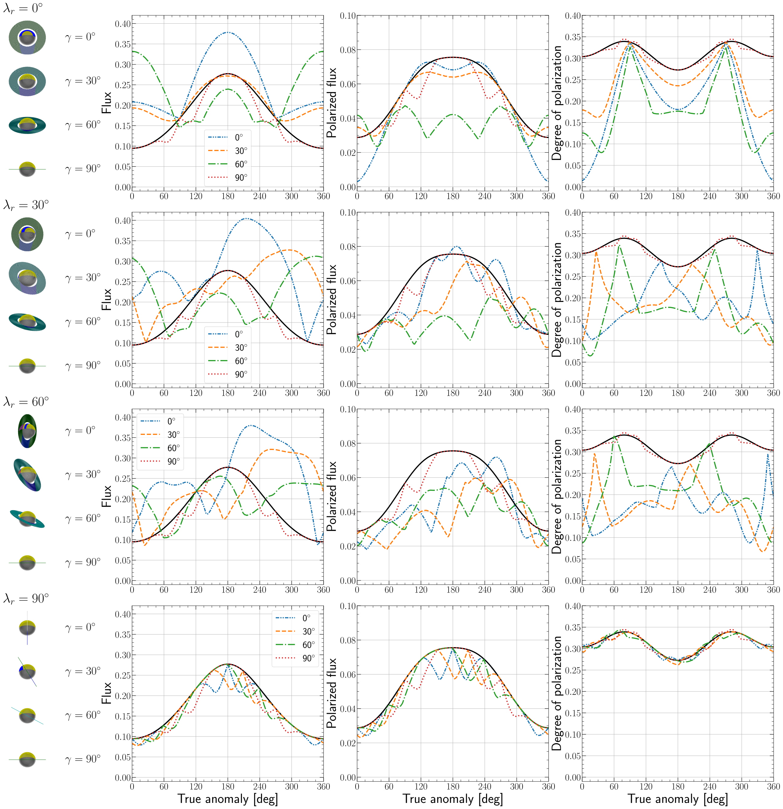
Figure 5: $F$ (left), $F_{\rm pol}$ (middle), and $P$ (right) of the light that is reflected by the model planet with a Saturn-like ring with $r_{\rm in}=1.2$ and $r_{\rm out}=2.25$, $b=1.0$, and $i=20^{\circ}$ ($\alpha_{\rm min}=70^{\circ}$ and $\alpha_{\rm max}=110^{\circ}$) as functions of the true anomaly $\nu$. The ring inclination longitude $\lambda_{\rm r}$ is 0^∘ (first row), 30^∘ (second row), $60^{\circ}$ (third row), and 90^∘ (bottom row). For $\lambda_{\rm r}=90^{\circ}$ the ring is ’seen’ edge-on. The ring inclination angle $\gamma$ is 0^∘ (blue, dash-dot-dot), 30^∘ (green, long-dashed), 60^∘ (red, long-dash-dot), or 90^∘ (purple, dot-dot). For $\gamma=90^{\circ}$, there is no dependence on $\lambda_{\rm r}$. The black lines are for the planet without a ring. The images on the left illustrate the planet with its ring at $\nu=0^{\circ}$, thus when it is closest to the observer.

Here we show the influence of the orientation of the ring for a given planetary orbital inclination angle $i$. To limit the number of plots, we use only two values for $i$, namely $20^{\circ}$ and $90^{\circ}$, with the first value representing a planetary system that would have been discovered using direct imaging, and the latter a system typically discovered using the transit method.

Figure 5 shows for $i=20^{\circ}$, $F$, $F_{\rm pol}$, and $P$ for ring inclination angles $\gamma$ of 0^∘ (a face-on ring), 30^∘, 60^∘, and 90^∘ (an edge-on ring), and for ring inclination longitudes $\lambda_{\rm r}$ of 0^∘, 30^∘, 60^∘, and 90^∘. Figure 6 is similar to Fig. 5 except for $i=90^{\circ}$. For comparison, the figures also include lines representing the ring-less planet. Most of the curves in Figs. 5 and 6 show angular features that are due to changing shadows (cf. Fig. 1). We will not discuss all features in detail but rather point out a few characteristic ones.

First, while the phase curves of the planet itself are symmetric around $\nu=0^{\circ}$, a non-zero ring inclination longitude $\lambda_{\rm r}$ makes them asymmetric. This has been noted before (Arnold & Schneider, 2004; Dyudina et al., 2005). For a given $i$, all curves with $\gamma=90^{\circ}$ (an edge-on ring) are the same, because the view on the ring is independent of $\lambda_{\rm r}$. In this edge-on orientation, the observer receives no light that has been reflected by or transmitted through the ring. However, the ring does leave traces in the light curves. For example, in Fig. 5 ($i=20^{\circ}$, and $\gamma=90^{\circ}$) the shadow the ring casts on the planet reduces $F$ and $F_{\rm pol}$ between approximately $\nu=50^{\circ}$ and $130^{\circ}$, and $230^{\circ}$ and $310^{\circ}$. For $\lambda_{\rm r}=90^{\circ}$, the ring is seen edge-on for all $\gamma$ and any difference with the ring-less planet curves is thus due to ring shadows. It is interesting to note that very few geometries allow the ring to go completely undetected. One such geometry is shown in Fig. 6 ($i=90^{\circ}$. When $\gamma=90^{\circ}$ the thin ring does not cast a shadow nor does it reflect (or transmit) light towards the observer. In fact, any configuration where the orbital inclination equals the ring inclination angle leaves the ring undetectable.

For all geometries, the curves of the ringed planets approach those of the ring-less planet at the ring-plane crossings, where the ring is illuminated on its edge and the shadow is infinitely narrow. Depending on its orientation, the ring can, however, still occult part of the planetary disk at the ring-plane crossings, leaving small differences between the curves, see for example in Fig. 5, the curve for $\lambda_{\rm r}=0^{\circ}$ and $\gamma=60^{\circ}$, where $F$ of the ringed planet is slightly lower than that of the ring-less planet at the ring-plane crossing. For $\lambda_{\rm r}=0^{\circ}$, the ring-plane crossings occur at $\nu=90^{\circ}$ and $270^{\circ}$ but for other values of $\lambda_{\rm r}$ and/or $\gamma$ (the latter only when $\lambda_{\rm r}\neq 0$), the locations of the ring-plane crossings are different.

The ring-plane crossings usually manifest themselves in the light curves as sharp changes which can be described as a discontinuity in the derivative due to the light suddenly having to travel through the ring. A prime example of such a discontinuity in Fig. 5 is the $\gamma=60^{\circ}$ curve at $\lambda_{\rm r}=0^{\circ}$. Between $\nu=0^{\circ}$ and $90^{\circ}$, the ring reflects light, strongly increasing $F$ of the planet-ring system compared to that of a ring-less planet. After the ring-plane crossing, the ring instead transmits light and casts a shadow on the planet, decreasing $F$ compared to the ring-less planet. The $\gamma=0^{\circ}$ curve in the same plot shows similar behavior but here the ring transmits and reflects along different parts of the orbit. The ring-plane crossings appear to be even more pronounced in $P$ than in $F$ and $F_{\rm pol}$.

Looking at the curves of $F_{\rm pol}$, it is clear that the light that is reflected or transmitted by the ring is usually less polarized than the light that is reflected by the planet. This suppresses $P$ of the system as a whole and is straightforward to understand from Fig. 3: the light that is singly scattered by the ring particles not only has a lower $P$, but at large scattering angles (small planetary phase angles $\alpha$) it also has an opposite direction of polarization compared to the light that is scattered in the planetary atmosphere, thus further decreasing $P$ of the whole.

The ring shadow on the planet can increase $P$ when it breaks the symmetry of the illuminated and visible planetary disk. Examples of this in Fig. 5 are the curves with $\gamma=90^{\circ}$: the edge-on ring prevents it from reflecting light to the observer, but $P$ is slightly higher just before and after the ring-plane crossings. Another example in Fig. 5 are the drops in the $P$-curves for $\gamma=60^{\circ}$ and $\lambda_{\rm r}=0^{\circ}$ and $30^{\circ}$ before and after the ring-plane crossings, where the ring casts its shadow on the planet.

The $F_{\rm pol}$-curves due to the ring are less straightforward to understand because they are not consistently lower than those of the ring-less planet. For example, in Fig. 5 for $\lambda_{\rm r}=30^{\circ}$ and $\lambda_{\rm r}=60^{\circ}$, the ring adds $F_{\rm pol}$ in the second part of the orbit. This is due to the high flux of the ring there, which even though it is only weakly polarized, still adds polarized flux to the total $F_{\rm pol}$. This effect is also visible in the $F_{\rm pol}$-curves in Fig. 6 for $\lambda_{\rm r}<90^{\circ}$ that show bumps at the beginning and end of the orbit.

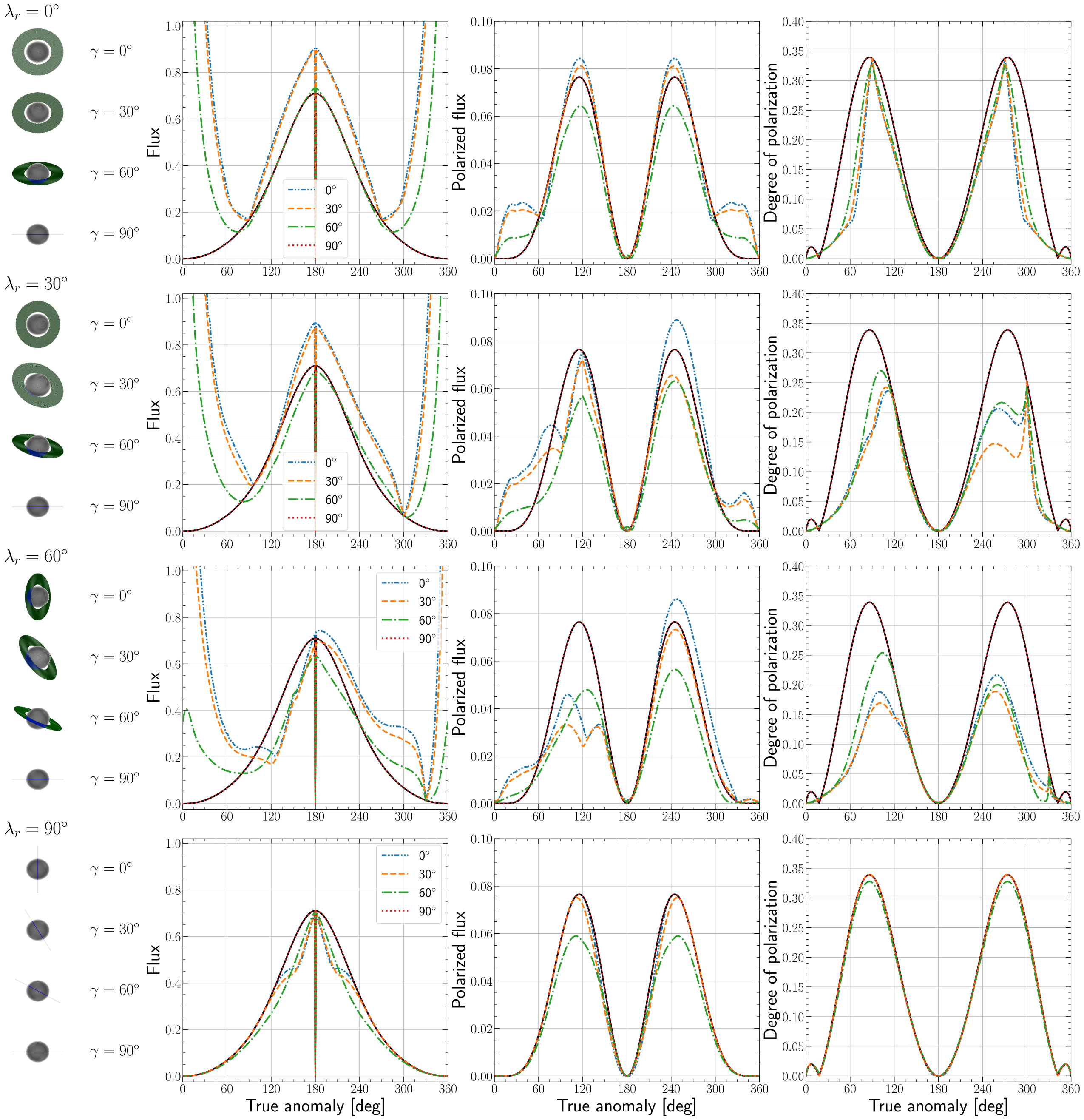
Figure 6: Similar to Fig. 5, except for $i=90^{\circ}$. The images on the left illustrate the system at $\nu=0^{\circ}$, which, for $i=90^{\circ}$, is precisely in front of the star, thus the nightside of the planet is turned towards the observer. To keep the structures in the curves visible, we have limited the vertical axis in the graphs for $F$, thus in some cases cutting off the forward scattering peaks. The missing peak values are the following: for $\lambda_{\rm r}=0^{\circ}$, the lines reach 6.13, 5.37, and 2.25 for $\gamma=0^{\circ},\ 30^{\circ}$, and $60^{\circ}$, respectively. For $\lambda_{\rm r}=30^{\circ}$, they reach 5.36, 4.61, and 1.55, and for $\lambda_{\rm r}=30^{\circ}$, 2.38 and 1.65 for $\gamma=0^{\circ}$ and $\gamma=30^{\circ}$, respectively.

For $i=90^{\circ}$ in Fig. 6, the ring is much brighter in diffusely transmitted light than in reflected light (note that the peak values of $F$ at small and large values of $\nu$ are mentioned in the figure caption). These peaks can be explained by the strong forward scattering peak in the single scattering flux of the ring particles (Fig. 3), especially in a part of the orbit where the planet itself is dark. It might seem that this forward scattering peak would easily be detectable for a planet-ring system. However, in this part of the orbit, the angular separation between the planet and its star is very small, which makes direct detections very hard. Such peaks could however be observable when monitoring the brightness of the star and variations therein. This has already been demonstrated by (Placek et al., 2014) in the infrared where hot giant planets are relatively bright but could possibly also be done at visible wavelengths (Sucerquia et al., 2020).

Changing the ring inclination longitude $\lambda_{\rm r}$ changes the locations of the ring-plane crossings but, unsurprisingly, not those of the forward scattering peak. The dramatic drops in $P$ that could be seen in Fig. 5 are also present in Fig. 6 but no longer significantly change the shape of the curves. Instead, the peak value of $P$ is often decreased, making it difficult to distinguish the curves from those of a ring-less planet. A ring-less planet with for example clouds could also significantly influence $P$ (see Stam et al., 2004; Karalidi et al., 2012). The asymmetry of the curves with $\lambda_{\rm r}=30^{\circ}$ could possibly help to identify the rings, although it would have to be ruled out that the asymmetrical behavior would be due to seasonal effects on a horizontally inhomogeneous ring-less planet as was remarked by Dyudina et al. (2005). Seasonal effects could, however, not explain the sharp changes due to the ring-plane crossings, in $F$ and $P$ at, for example, $\nu=300^{\circ}$. Such sharp changes, which would require frequent observations of the system would be valuable characterizing features to search for.

4.3 The influence of the ring optical thickness

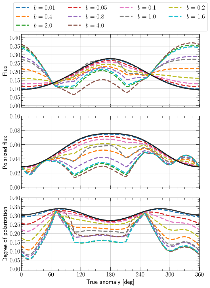
Figure 7: $F$ (top), $F_{\rm pol}$ (middle), and $P$ (bottom) as functions of $\nu$ for ring optical thicknesses $b$ ranging from 0.01 (dark blue) to 4.0 (brown). For this planet-ring system, $i=20^{\circ}$, $\lambda_{\rm r}=30^{\circ}$, $\gamma=60^{\circ}$, $r_{\rm in}=1.20$, $r_{\rm out}=2.25$, and $\varpi=0.8$. The black line represents the ring-less planet.

Figure 7 shows the influence of the ring optical thickness $b$ on the signals of the standard planet-ring system. First, we’ll discuss the influence of $b$ along the part of the orbit where the ring reflects incident light, and then the more complicated part where the ring diffusely transmits light.

In the figure, the ring reflects light for $\nu\leq 69.4^{\circ}$ or $\geq 249.4^{\circ}$ and with that generally increases $F$ of the system as a whole. The increase in $F$ increases with $b$, although not linearly. With increasing $b$, the increase in $F$ vanishes as the reflection by the ring reaches an asymptotic value when increasing $b$ does not further increase $F$. Note that along this part of the orbit, the planet also casts its shadow on the ring, thus decreasing the ring-contribution to $F$, while the ring hardly casts a shadow on the planet.

In reflected light, polarized flux $F_{\rm pol}$ of the system is lower than that of the ring-less planet at small values of $\nu$, while it is larger at large values of $\nu$, with the difference increasing with $b$ and converging for the larger values of $b$. The reason for the lower and higher values of $F_{\rm pol}$ when the ring is added are due to the polarized flux of the light that is singly scattered by the ring particles, which has an opposite direction of that of the gas molecules in the planet’s atmosphere at the small values of $\nu$, where the single scattering angle $\Theta$ is larger than 150^∘, and the same direction at the large values of $\nu$, where $\Theta$ is smaller than 150^∘ (see Fig. 3).

Between $69.4^{\circ}<\nu<249.4^{\circ}$, the ring diffusely transmits light, adding to the total flux of the system. At the same time, the ring casts shadows on the planetary disk en occults part of the disk, both effects suppressing the planetary flux (see Fig. 1). To understand the relation between the transmitted light and $b$, Fig. 8 shows $F$, $F_{\rm pol}$, and $P$ of diffusely transmitted light of just a slab of ring-material for a viewing angle of $0^{\circ}$, different angles of incidence, as functions of $b$. As can be seen, the curves for $F$ increase with $b$ due to increased scattering of light by the ring particles (the flux of the directly, thus non-scattered beam of light decreases with increasing $b$), until about $b=1$ to 3 (depending on $\theta_{0}$ and $\theta$ as those angles affect the effective ring optical thickness). Further increases of $b$ decrease the diffusely transmitted $F$ as fewer and fewer photons get through the ring.

The relative large values of $F$ between $\nu\approx 100^{\circ}$ and $210^{\circ}$ in Fig. 7, are due to the changing size of the planet shadow on the ring. Similar behavior can be seen for $F_{\rm pol}$.

The degree of polarization $P$ generally decreases with increasing $b$ as the amount of multiple scattered, generally low polarized, light, increases with $b$. Between $\nu=69.4^{\circ}$ and $249.4^{\circ}$ where the flux of the reflected ring-light is small, this depolarizing effect is not very prominent, especially not for $b=4.0$: the very small ring-flux hardly contributes to $F$ and $F_{\rm pol}$ while at the same time, the ring strongly shadows and occults the planet and thus also decreases the total flux of the system.

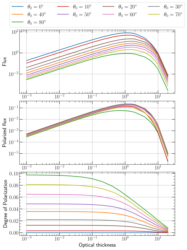
Figure 8: The diffusely transmitted $F$ (top), $F_{\rm pol}$ (middle), and $P$ (bottom) as functions of the optical thickness $b$ of a slab of ring-material for illumination angles $\theta_{0}$ ranging from 0^∘ (blue) to 80^∘ (green). The viewing angle $\theta$ is $0^{\circ}$.

4.4 The influence of the single scattering albedo

Next, we vary the single scattering albedo $\varpi$ of the ring particles to mimic different particle compositions. The icy particles surrounding Saturn would, for example, not survive at the distance between the Earth and the Sun. Considering the recent discoveries of puffed-up planets, of which the transit depth combined with their mass would indicate very small densities, that could possibly be explained by the presence of a ring (Piro & Vissapragada, 2020) as that could increase the transit depth, it is important to also look at refractory materials (which have a lower albedo in the visible) (Piironen et al., 1998; Ostrowski & Bryson, 2019).

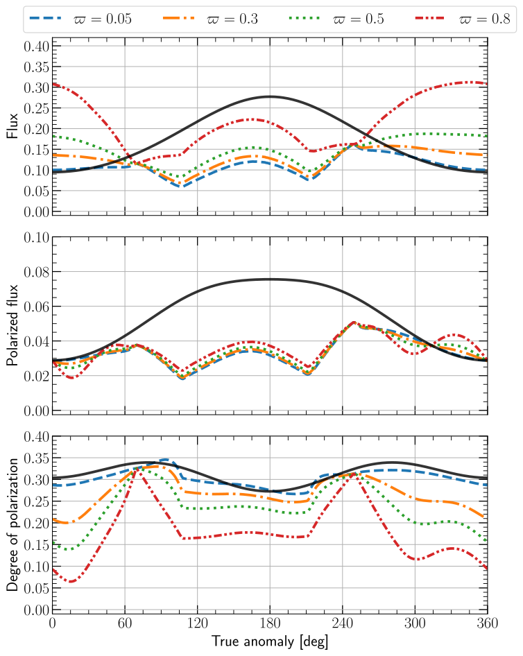
Figure 9: Similar to Fig. 7, except for different single scattering albedos $\varpi$ of the ring particles: 0.05 (blue, dashed), 0.3 (orange, dashed-dot-dot), 0.5 (green, dotted), and 0.8 (red, short-dashed-dotted). The system-parameters are $i=20^{\circ}$, $\lambda_{\rm r}=30^{\circ}$, $\gamma=60^{\circ}$, $r_{\rm in}=1.20$, $r_{\rm out}=2.25$, and $b=1.0$.

Figure 9 shows $F$, $F_{\rm pol}$, and $P$ for the standard planet-ring system and $\varpi$ ranging from 0.05 to 0.8. Not surprisingly, increasing $\varpi$ increases $F$, regardless of whether the ring is seen in reflected or transmitted light. Because for a given $b$, $\varpi$ has no effect on the shadowing or occultation by the ring, and because the single scattering polarization of the particles is independent of $\varpi$, $F_{\rm pol}$ shows little dependence on $\varpi$, indirectly showing how small the contribution of the ring is to $F_{\rm pol}$ of the system. The variation in $P$ is thus mostly due to the variation in $F$.

From comparing Figs. 7 and 9, we conclude that for this planet-ring system, it is difficult to determine whether a curve would be due to a larger value of $b$ or a higher value of $\varpi$. Increases in either parameter lead to higher fluxes when the ring is reflecting light and a larger $b$ can also increase the transmitted flux. For a different orientation of the ring and/or planetary orbit, this might be different, however, and that is something that should be studied with a full retrieval algorithm applied to simulated curves.

4.5 The influence of the ring radius

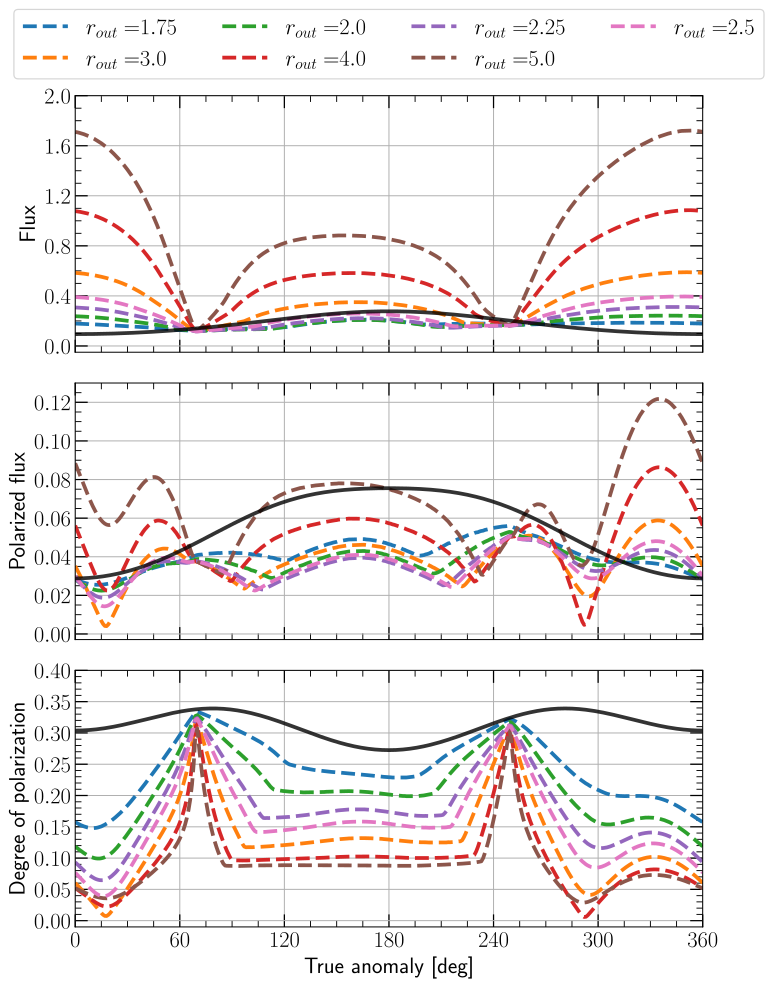
Figure 10: Similar to Fig. 7, except for different outer ring radii $r_{\rm out}$ (expressed in planet-radius $r$): 1.75 (blue), 2.0 (green), 2.25 (purple), 2.5 (pink), 3.0 (orange), 4.0 (red), and 5.0 (brown). The system-parameters are $i=20^{\circ}$, $\lambda_{\rm r}=30^{\circ}$, $\gamma=60^{\circ}$, $r_{\rm in}=1.2$, $\varpi=0.8$, and $b=1.0$.

The influence of the outer ring radius $r_{\rm out}$ is shown in Fig. 10. The curves are very similar to those for various ring optical thicknesses $b$ (Fig. 7) since increasing $r_{\rm out}$ increases the reflected fluxes and, depending on the geometry, also the shadows in a similar way as increasing $b$ does. There are some key differences, however. For example, along parts of the orbit where the ring is diffusely transmitting light, the ring flux increases with increasing $r_{\rm out}$ while it would decrease with increasing $b$ beyond a value of about 1.0 (see Fig. 8).

Another difference compared to changing $b$ is found in the curves for $F_{\rm pol}$: while increasing $b$ decreases $F_{\rm pol}$ of the system as a whole, because light that has been scattered multiple times is less polarized, there is no such relation with the ring size: the larger $r_{\rm out}$, the larger the $F_{\rm pol}$ that is added to the signal of the planet-ring system. With increasing $r_{\rm out}$, the curves for $P$ converge as the polarization signal of the rings starts to dominate that of the planet (except near the ring-plane crossings). This trend is helped by the fact that eventually, increasing $r_{\rm out}$ no longer increases the extent of the shadows on the planet.

The dips around $\nu=15^{\circ}$ and $290^{\circ}$ become more pronounced when the ring brightens as is evident from Figs. 7, 9, and 10. At these locations in the orbit, the angle of polarization of the ring-light is opposite to that of the planet-light, thus decreasing $P$; an effect that becomes more prominent with increasing $r_{\rm out}$. For $r_{\rm out}=5.0$, the flux that is reflected by the ring dominates the planetary flux and $P$ no longer approaches zero.

5 The case of HIP 41378 f

As a case study, we simulate the flux and polarization signals of “puffed-up” planet HIP 41378 f (Akinsanmi et al., 2020b; Alam et al., 2022), assuming that it is not a single planet, but a planet with a ring. HIP 41378 f is suspected to have a ring because of its extremely small average density of $0.09\pm 0.02$ g cm^-3 that follows from fitting the transit with a ring-less planet. A follow-up study by Alam et al. (2022) showed that the hypothesis of a ring holds up when the observations are done over a range of wavelengths but so does the hypothesis of an extended atmosphere. Assuming that the transit depth is partly caused by a ring, Akinsanmi et al. (2020b) find an average density $\rho_{\rm p}$ of $1.2\pm 0.4$ g cm^-3 instead.

HIP 41378 f has a relatively large semi-major orbital axis of about 1.4 AU that, at a distance of 103 pc, translates to a sky-projected angular separation with its F-type parent star of $\sim$13 mas (Santerne et al., 2019). This would be large enough to resolve the planet by direct imaging telescopes like the proposed Large UV/Optical/Infrared Surveyor (LUVOIR) (The LUVOIR Team, 2019). The planet has an equilibrium temperature $T_{\rm eq}$ of $\sim$294 K (assuming a bond albedo of zero, Santerne et al. 2019), so there will be no significant thermal emission that would mix in with the reflected starlight and decrease the planet’s degree of polarization $P$. The transit of HIP 41378 f has been observed as part of the K2-mission (Howell et al., 2014) which observed at visible wavelengths that are comparable to the 633 nm that we used for our previous computations.

Table 2: HIP 41378 f parameters (without uncertainties) as derived by Akinsanmi et al. (2020b). The orientation of the ring is defined differently by Akinsanmi et al. (2020b) so our values for $\gamma$ and $\lambda_{\rm r}$ are different than theirs for the same ring orientation. $r_{\rm p}$ is the planet radius (expressed in Earth radius $r_{\oplus}$), $a$ is the orbital semi-major axis, $r_{*}$ is the stellar radius.

Parameter	Value
$r_{\rm p}$ [$r_{\oplus}$]	3.7
$a/r_{*}$	231.0
$i$ [∘]	89.97
$r_{\rm in}$ [$r_{\rm p}$]	1.05
$r_{\rm out}$ [$r_{\rm p}$]	2.6
$\gamma$ [∘]	-2.11
$\lambda_{\rm r}$ [∘]	-24.92

A detailed fit of the transit using Pryngles is outside the scope of this study. Instead, the results presented in this section demonstrate the capabilities of Pryngles and provide an estimate of the detectability of the reflected light signals of this system. The parameters of a ringed planet that were determined by (Akinsanmi et al., 2020b) are shown in Table 2. In order to show the detectability of the reflected light, we will use extremes of the ring optical thickness $b$ and the single scattering albedo $\varpi$ of the ring particles that are possible within the constraints of the values in Table 2. Especially $\varpi$ is unconstrained by the transit but can have significant influence on the reflected flux (see Fig. 9). We will use values of $\varpi$ equal to 0.05 and 0.8 (see Fig. 9) where we note that a value of 0.8 is high for the ring particles as they presumably consist of rocky material considering the proximity to the star. Both Akinsanmi et al. (2020b); Alam et al. (2022), however, derive an average density $\rho$ of the ring particles of $1.08\pm 0.3$ g cm^-3, which is low compared to most rocky materials. This can be explained by porous materials (Carry, 2012) or ice that is continuously being deposited by an unknown source.

Furthermore, both Akinsanmi et al. (2020b) and (Alam et al., 2022) assume an opaque ring. While this assumption is not realistic, model simulations show that for $b\geq 4$, the transit depth would be fairly close to the observations. Therefore, we vary $b$ between 4 and 20, large enough values to be considered an opaque ring. The orientation and ring radius are a much more direct result of the transit fit, and we’ll thus adopt the values derived from the fit (Table 2). We again use the scattering properties of the olivine particles that are comparable in size to the particles that were used in the follow-up study by (Alam et al., 2022). For simplicity, we use the same gaseous planetary atmosphere as before.

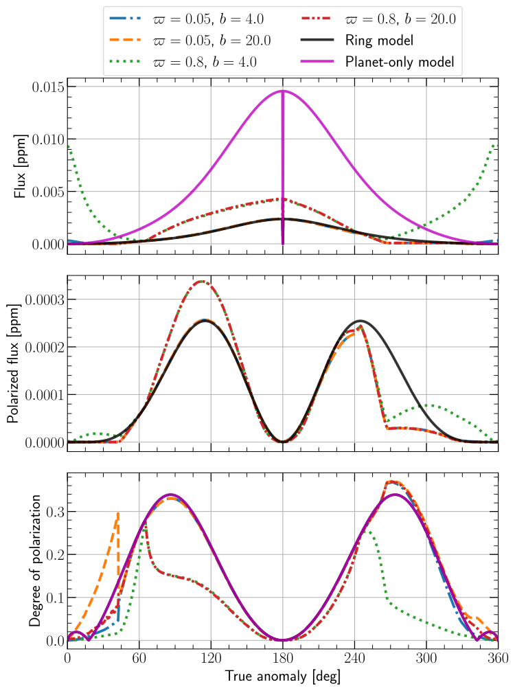
Figure 11: $F$, $F_{\rm pol}$, and $P$ of HIP 41378f for different values of $b$ and $\varpi$ as functions of $\nu$. The magenta curves pertain to the ring-less, ”puffed-up” planet and the black curves to the ringed-planet model but without a ring, using the parameter values of Akinsanmi et al. (2020b). All curves use the same orbital inclination and stellar properties but the magenta curve has a different semi-major axis ($a/r_{*}=231.6$). In the $F_{\rm pol}$-plot, the magenta curve has been omitted as it has the same shape as the black curve except with maximum values up to   0.0015 ppm. In the $P$-plot, the magenta and black curves overlap.

Figure 11 shows $F$, $F_{\rm pol}$, and $P$ for the various model planets and rings. It can be seen that even in the most favorable case, the contrast required to detect the planet with rings is on the order of $10^{-9}$. This is not attainable with SPHERE/ZIMPOL (Thalmann et al., 2008) or even with JWST (Carter et al., 2022), especially at the small angular separation for the maximum flux of 13 mas. If this contrast and resolution can be achieved in the near-future, we would be able to distinguish between a ring-less or a ringed planet. Note that the large spike in $P$ before $\nu=60^{\circ}$ would not be observable due to the low $F$ at that location in the orbit.

If we take the curve for the planet-only model as unknown in exact brightness but having the presented shape, then it becomes clear that at least two measurements are necessary to reliably differentiate between the two models. Considering the angular separation is largest around $\nu=90^{\circ}$ and $270^{\circ}$ the focus should be on differences in that region. Luckily, this is also where the biggest differences are in both $F$ and $P$. If there is a ring, a flux difference would be found when measuring at $\nu=90^{\circ}$ and $270^{\circ}$ which would not be the case for the ring-less planet. This flux difference is there regardless of the optical thickness or single scattering albedo of the ring but could be absent or changed if the ring has a different orientation. If the polarization of the light is also measured, something could be said about the composition of the ring. For example, assuming that the ring is truly opaque, so $b=20$, $P$ at $\nu=90^{\circ}$ would be a function of $\varpi$ and so could potentially be extracted. A thorough analysis of observations could extract both the optical thickness and albedo based on the difference in $P$ at $\nu=90^{\circ}$ and $270^{\circ}$.

Based on these results it should be possible to distinguish between a planet with a simple atmosphere and a planet with a ring if they could be directly observed. If $P$ is also measured it should even be possible to extract some of the properties of the ring. As was mentioned in Sect. 4.2 and by Dyudina et al. (2005), a planet that shows seasonal activities might also produce asymmetrical light curves. A follow-up study could investigate this possibility based on the proposed atmospheres by Alam et al. (2022). A third possible explanation comes from a recent study that shows that the observed transit can be explained by the presence of an exomoon (Harada et al., 2023). The reflected light of a planet with an exomoon could in theory also lead to a measured flux difference because the moon may move in front of the planet, or vice versa. The chance of this happening during an observation depends on the size and period of the moon as well as the observation frequency but should be small, as was shown by Berzosa Molina et al. (2018b). They also showed that such transits (of the moon in front of the planet or vice versa) only result in shallow, brief dips in the light curve. The dips were especially small in the curves for $P$ (around $2\%$) and so should be distinguishable from the effects of a ring.

6 Discussion

The work presented here provides significant enhancements to the current state of the art in light scattering and polarization modeling compared to Lietzow & Wolf 2023. Our model uses a scattering matrix based on measurements of real particles and, perhaps more importantly, is a publicly available package Pryngles. Furthermore, our study explores different orbit orientations and considers the case of an actual planet, HIP 41378 f, which has an extremely low density, making it a prime candidate for reanalysis under the ringed planet model (Zuluaga et al., 2015; Akinsanmi et al., 2020b). The particles that we used have more realistic scattering behavior than similarly sized spherical particles but also have properties that are not found in ring particles, such as the material that they are made of. For example, the rings of Saturn are mainly composed of icy materials (Cuzzi et al., 1984) and have a different refractive index compared to the olivine particles that were used. In future updates, different ring particles will be added to the package based on data in the Amsterdam-Granada database (Muñoz et al., 2012b). Another potential problem is that the used particles have a log-normal distribution (Muñoz et al., 2000; Moreno et al., 2006) while ring particles have a power-law distribution (Dohnanyi, 1969; Cuzzi & Pollack, 1978). The difference in scattering behavior of the two different size distributions should be investigated in a future study. The effect of non-homogeneous rings should also be explored in a future study as our model ring is horizontally homogeneous, while real planetary rings, such as those in the solar system, are not. The rings in our solar system exhibit azimuthal variations, but especially radial variations in their optical thickness and particle properties. Such inhomogeneities will influence the ring shadows and occultations, and their traces in the signals of planet-ring systems would be interesting to explore.

In general, the developments presented here can contribute to three fronts in the search for exoplanets with rings: rings around exoplanets in close-in orbits (i.e. ”warm exorings”), circumplanetary disks (CPDs), and rings around distant giant planets similar to Saturn’s rings. With respect to the first case, populations of warm rings, proposed originally by Schlichting & Chang 2011, can exist in proximity to their host stars for millions of years and will be composed of refractory particles rather than icy particles as in Saturn’s rings. The thermal emission of warm rings cannot be modeled using our model but when computing flux or the degree of polarization, it could be added as a constant flux because the thermal emission is predicted to have a relatively low degree of polarization (Stolker et al., 2017). Because our scattering model as presented here is based on irregular olivine particles which, while they may not necessarily be found in rings, can represent refractory particles, our model can be used to model the reflected light.

In the second case, massive planets with extensive orbits have a higher likelihood of developing substantial circumplanetary disks, which may ultimately transform into planetary rings upon completion of the satellite formation process. The detection of such planet-ring systems could be achieved using high-contrast imaging techniques, which are the sole method of planet detection that offers spatial resolution of photons emanating from planets and their surroundings (See, e.g. Ruane et al., 2018). This approach utilizes coronagraphs or other nulling methods to suppress light from the central star, and in conjunction with observing techniques such as Angular Differential Imaging (ADI), can attain contrasts of 10^-6 at separations of tenths of arcseconds (Marois et al., 2010). Consequently, this method enables the detection of self-luminous gas giants (i.e. planets that are still forming) on wide orbits and the effects of their presumed rings. To date, planets identified using direct imaging are generally a few million years old and situated tens of astronomical units from their host star favoring the survival of icy rings. High-contrast imaging has yielded several significant discoveries, including the detection of four planets orbiting HR 8799 (Marois et al., 2010), the planet $\beta$ Pic b (Lagrange et al., 2010), and others. As a result, the advancements presented in this paper demonstrate a potential for modeling the circumplanetary ring populations discovered through the aforementioned techniques.

Although Pryngles can handle eccentric orbits, we assume circular orbits to reduce the number of free parameters. Also, our results can be scaled for eccentric orbits by multiplying the total and polarized fluxes by a factor to represent the actual incident fluxes on the planet and its ring (the degree of polarization of the reflected signal would be unaffected by the orbital eccentricity). A potential complexity with simulating a ringed planet in an orbit with a large eccentricity is that depending on the size of the rings and the semi-major axis of the orbit, the illumination angle might no longer be uniform across the ring, while we assume a single illumination angle across the ring.

Our numerical predictions could not be compared against real observations of an actual ringed planet such as Saturn, because ground-based telescopes (or space telescopes in the vicinity of Earth), can only observe these planets at small phase angles, where the degree of polarization of the reflected light is very small because of a symmetric geometry. Observing these planets as if they were exoplanets is only possible with an orbiter, such as the Cassini spacecraft that orbited Saturn, or a fly-by mission. However, although Cassini’s Imaging Science Subsystem (ISS) instrument had polarimetric capabilities (Porco et al., 2004), no polarimetric observations of Saturn and its ring system have been published as of yet (West, 2022).

Polarimetry could also be a valuable method for detecting and characterizing the magnetic fields of ringed exoplanets. As in the case of the giant planets in the Solar System (and in the debris disks around young stars), a planet’s magnetic field can modify the optical properties of the rings by influencing the particle orientations (Dollfus, 1984; Lazarian, 2007). Finding ring particle orientations could thus potentially provide valuable information about the structure and dynamics of the planet’s interior, which in turn could provide clues about the habitability of these worlds (in case of rocky planets) and their satellites (see, e.g. Heller & Zuluaga 2013, and references therein).

Lastly, the study of light scattered from planetary rings around exoplanets is highly relevant to the current search for Saturn-like planets, and their characterization can reveal important information about their evolution and their environments. The modeling of the scattering and polarization of dust grains in planetary rings can provide valuable insights into the composition and evolution of the rings themselves, as well as the dynamics of the planet-ring system as a whole. Our study contributes to this field by providing a more accurate and realistic scattering model, which can be used in conjunction with high-contrast imaging techniques to search for and characterize exoplanet ring systems. By improving our understanding of the optical properties of planetary rings, we can gain further insights into the formation and evolution of exoplanet systems, and potentially identify new targets for future and ongoing missions such as the LUVOIR and the James Webb Space Telescope.

7 Summary and Conclusions

We have computed the effects of a ring around an extrasolar planet on the total and polarized fluxes of starlight that is reflected by the planet-ring system as a whole. For these computations, we extended the python package Pryngles with an adding-doubling radiative transfer algorithm that includes all orders of scattering and polarization (de Haan et al., 1987). We assumed dusty rings that are comprised of irregularly shaped particles with an effective radius of 1 $\mu$m. By varying system parameters, we investigated their role on the system’s flux and polarization light curves. The system parameters that we varied are the ring orientation (Sect. 4.2), the ring optical thickness (Sect. 4.3), the single scattering albedo of the ring particles (Sect. 4.4), and the outer ring radius (Sect. 4.5. To put the results into context we also performed a simple case study of the possibly ringed planet HIP 41378 f (Sect. 5).

Our computations show a number of features indicative of a ring. In general, a ring (that is not seen edge-on), leaves two (different) peaks in the total flux of the system flux curve, with one due to the light that is reflected by the ring and the other due to the diffusely transmitted light. This was also reported by Arnold & Schneider (2004) and Dyudina et al. (2005). Including polarization, however, allows us to expand upon this and show that the increase in flux due to the ring that caused the second peak has a substantially lower degree of polarization. The lower degree of polarization of the light reflected or transmitted by the ring comes from the difference between molecules and particles and is therefore almost always present. This dichotomy between higher flux but a lower degree of polarization is therefore a key signature of a ring and was also reported in a recent study by Lietzow & Wolf (2023). A notable exception to this would be a planet that shows large, seasonal activity, as was presented by Dyudina et al. (2005) (without polarization). What sets the effect of rings apart from such a planet are the large changes in flux and degree of polarization around the ring-plane crossings, when the ring is illuminated edge-on. Therefore these sharp changes in the flux and degree of polarization curves would be something to look for in future observations. Lastly, due to the occultation of the ring in front of the planet or the shadow cast onto the planet, the received flux can be lower than expected, even when the ring is seen edge-on.

While each of the system parameters that were varied has distinct effects on the light curve we demonstrated that there is also a big overlap between them. Especially when it comes to the properties of the ring such as optical thickness, particle albedo, and size. Some of these properties, like the size of the ring and its optical thickness, also have an effect on the stability of the ring. So in order to draw a good conclusion, future observations should perform thorough fits of the parameter space to extract as much information as possible. Such a fit should include eccentric orbits, which is already possible using Pryngles, and different planetary atmospheres as was done by Lietzow & Wolf (2023), which is not yet possible. The variation of the latter is interesting to combine with observations in different wavelength bands, in particular at wavelengths where gases in the planetary atmosphere absorb, and where the planet is thus dark, which could highlight the presence of rings and help to characterize them.

The case study showed that it is currently impossible to directly observe such a system, it might be with the next generation of space telescopes like LUVOIR (The LUVOIR Team, 2019), HabEx (Gaudi et al., 2018), or the recently by NASA announced Habitable Worlds Observatory (HabWorlds or HWO). We show that it would indeed be beneficial for those missions to use polarimetry as it allows for the identification of properties like the optical thickness and particle albedo of exorings, something not possible using only flux measurements.

We conclude that a ring leaves unique features in the reflected and polarized fluxes of a planet as it orbits its star. In order to identify rings, observations along the planetary orbit would be needed, in particular aiming to cover the ring-plane crossings, where sharp changes in the system’s signals should be detectable. Combining photometry and polarimetry would help to characterize the physical properties of rings, such as their size, orientation, and optical thickness, which would allow us to better understand planet formation and the formation and evolution of the rings around the planets in our Solar System.

Appendix A Calculating the angles associated with the spangles

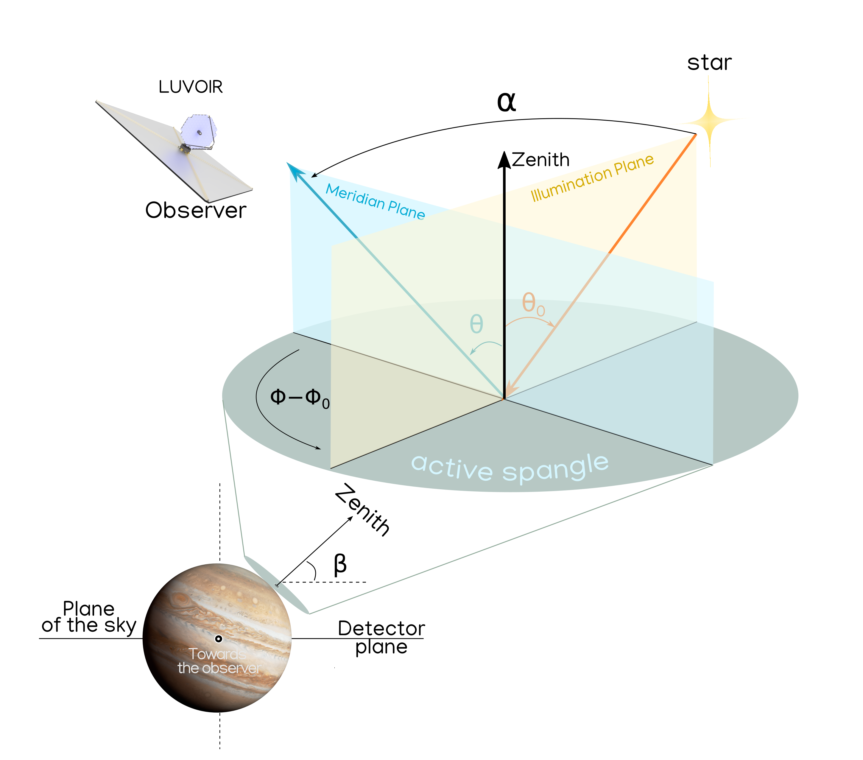
Figure 12: Spangle geometry: orientation and angles involved in the calculation of stellar light scattering by an individual spangle, along with the observer’s orientation (here, a LUVOIR-type telescope is the observer).

In Fig. 12 we show the geometry of light scattering for a single spangle. For each spangle, we have to compute the local stellar zenith angle $\theta_{0}$, defined as the angle between the local zenith direction and the direction towards the star; the local viewing zenith angle $\theta$, which is the angle between the local zenith direction and the direction towards the observer; and the local azimuthal difference angle $\phi-\phi_{0}$, taken as the angle between the plane that contains the direction towards the local zenith and the direction towards the observer, and the plane that contains the direction towards the local zenith and the direction of propagation of the incident starlight. Angle $\phi-\phi_{0}$ is measured rotating in the clockwise direction when looking towards the local zenith (see de Haan et al. 1987). For a description of our computation of $\phi-\phi_{0}$, see Appendix D.

In all cases, we assume that the incident direction of the starlight is the same across the planet and the ring (the local incident angles depend of course on the spangle). This assumption would not hold for computations for planets with very wide rings and/or that are very close ($\ll 0.1$ AU) to their star.

Given angles $i$, $\gamma$, and $\lambda_{\rm r}$ (which are part of the user-provided input to the package), Pryngles computes, for each $\nu$ along the planetary orbit, the phase angle $\alpha$, and for each spangle on the planet and the ring, the angles $\theta_{0}$, $\theta$, and $\phi-\phi_{0}$. Note that unlike the planet spangles, all ring spangles have the same illumination and viewing geometries at a given value of $\nu$. Then, taking into account the radius of the planet, the inner and outer radii of the ring, and the direction to the star, Pryngles computes the state of the spangle, namely, whether it is illuminated by the star and visible to the observer; whether it is in the shadow of the ring (for planet-spangles) or the planet (for ring-spangles); and/or whether it is occulted by the ring (for planet-spangles) or the planet (for ring-spangles) (for a discussion on the key concept of “spangle state” in Pryngles, see the original paper by Zuluaga et al. 2022).

Appendix B Calculating the ring-plane crossings

The location of the ring-plane crossings can be calculated by solving

$${\bf n}_{\rm r}\cdot{\bf n}_{\rm star}(\nu_{\rm rp})=0\ ,$$ (12)

with ${\bf n}_{\rm r}$ the normal vector to the ring, $\nu_{\rm rp}$ the true anomaly of the ring-plane crossings. and ${\bf n}_{\rm star}$ the normal vector pointing from the planet to the star. We may express these locations in terms of the key angles:

$$\sin{(\lambda_{\rm r})} \cos{(\gamma)}\sin{(\nu_{\rm rp})}\ +$$

$$\cos{(\nu_{\rm rp})}\ \Bigl{[}\cos{(\lambda_{\rm r})}\cos{(\gamma)}\sin{(i)}-\sin{(\gamma)}\cos{(i)}\Bigl{]}=0.$$

In Fig. 1, for instance, where $\lambda_{\rm r}=0^{\circ}$, the crossings occur at $\nu=90^{\circ}$ and 270^∘ (the rings are colored white there).

Appendix C Comparison with a Lambertian reflecting planet

To validate the correct implementation of disk integration and geometry the total reflected flux is compared against the analytical expression for the phase function of a Lambertian reflecting planet with a surface albedo of $A_{s}$,

$$F(\alpha)=\frac{2A_{s}}{3\pi}\left(\sin{\alpha}+(\pi-\alpha)\cos{\alpha}\right).$$ (13)

In figure 13 this theoretical model, with a surface albedo of 1.0, is compared to a Lambertian reflecting planet modeled by Pryngles. The differences are very small and also show no systematic errors.

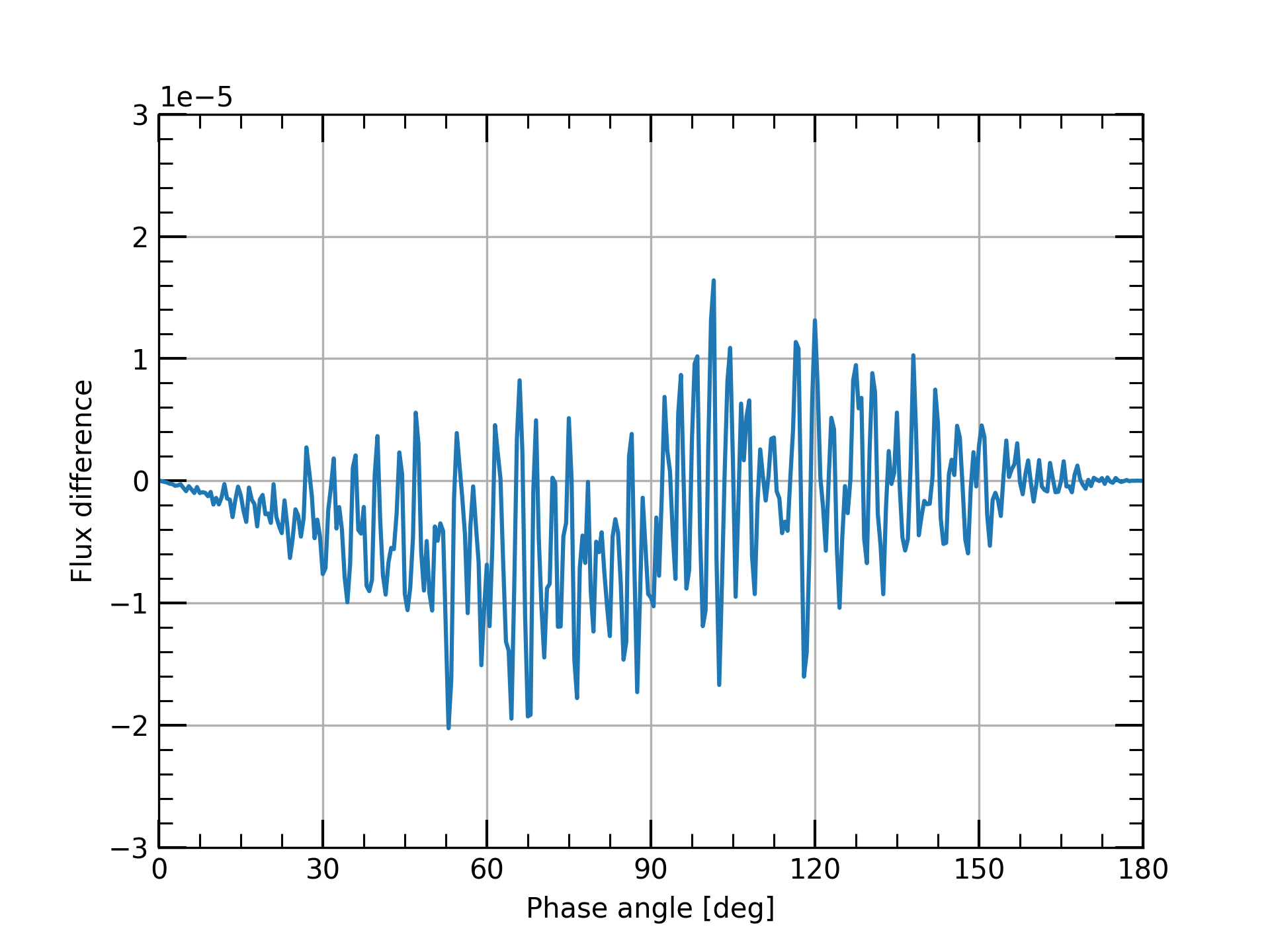
Figure 13: Difference in flux between theory and model for a Lambertian planet with 10,000 spangles.

Appendix D Computing $\phi-\phi_{0}$ and $\beta$

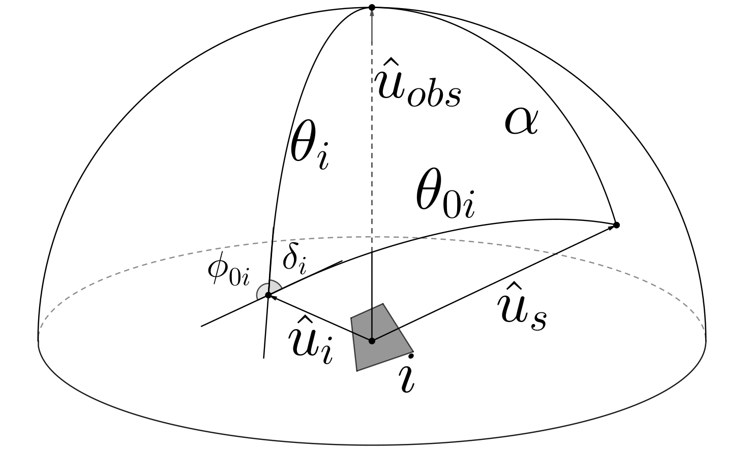
Figure 14: The angles and unit vectors associated with each individual spangle $i$. They are: the phase angle $\alpha$, direction to observer $\hat{u}_{\rm obs}$, direction to the star $\hat{u}_{\rm s}$, normal vector $\hat{u}_{i}$, illumination angle $\theta_{i,0}$, viewing angle $\theta_{i}$, azimuthal angle $\phi_{0,i}$, and intermediate angle $\delta_{i}$. The rotation angle $\beta_{i}$ is not shown here.

We describe here the calculations for $(\phi-\phi_{0})$ and $\beta$ in more detail. Starting with the azimuthal difference angle, and followed by the reference plane rotation angle $\beta$.

The azimuthal angles ($\phi$ and $\phi_{0}$) can be defined with respect to any plane containing the local z-axis which makes the plane that also contains the observer an obvious choice since this eliminates one of the two angles that need to be calculated, namely $\phi$. Thus an expression is needed for $\phi_{0}$ which then automatically also becomes an expression for $\phi-\phi_{0}$. Using the spherical law of cosine an expression can be found for an intermediate angle we name $\delta$ which is used to find $\phi_{0}$ with respect to the plane containing the direction to the observer and local z-axis,

$$\phi_{i,0} =\pi-\delta_{i}\ ,$$ (14)

$$\delta_{i} =\arccos{\left(\frac{\cos{\alpha}-\cos{\theta_{i,0}}\cos{\theta_{i}}}{\sin{\theta_{i,0}}\sin{\theta_{i}}}\right)}\ ,$$ (15)

where the subscript $i$ stands for the $i^{\text{th}}$ spangle.

Care has to be taken, however, in making sure the angle that is found using the above equation is for a rotation that is clockwise when looking in the positive local zenith direction. Whether the found angle needs to be adjusted depends generally on the orientation of the spangle, be it planetary or ring, and the direction of the star-light. The dependency on the location of the star can be understood from Fig. 14 where $\alpha$ will change during the orbit, eventually moving to the other side of the plane formed by $\hat{u}_{i}$ and $\hat{u}_{obs}$, the normal vector of the spangle and the normal vector pointing to the observer respectively. For planetary spangles, the angles are modified as

$$(\phi_{i}-\phi_{i,0}) =\phi_{i,0}\ ,$$ (16)

$$(\phi_{i}-\phi_{i,0}) =-\phi_{i,0}\ ,\quad\text{if}\quad y_{i}^{scat}<0\ ,$$ (17)

with $y_{i}^{scat}$ the $y$-location of the spangle with respect to the planetary scattering plane. Where the criterion there is to compensate for the flipping of the normal vector for spangles on the ”southern” hemisphere. The dependency on the location of the star is already incorporated into the $y$-location with respect to the planetary scattering plane.

Since all ring spangles have the same normal vector there is no dependency on their location on the ring. There is, however, a dependency on the orientation of the ring since it determines the locations in the orbit where the flip in the rotation direction happens. The locations of these flips are defined as the place where the plane containing the star, the planet, and the observer and the plane containing the normal vector of the ring and the observer are parallel. A 2D projection of the problem is shown in Fig. 15 with the two vectors in the direction of the star $\hat{u}_{\text{star, (1,2)}}$ representing two moments in the orbit.

Two situations arise, depending on the orientation of the ring. If the normal vector of the ring $\hat{u}_{\text{ring}}$ is pointing in the ${}^{+}y$ direction,

$$(\phi_{i}-\phi_{i,0})=-\phi_{i,0}\ ,$$ (18)

when the vector pointing to the star $\hat{u}_{\text{star}}$ is on the ${}^{-}x$ side of the plane formed by $\hat{u}_{\text{ring}}$ and the observer. If $\hat{u}_{\text{ring}}$ is pointing in the ${}^{-}y$ direction,

$$(\phi_{i}-\phi_{i,0})=-\phi_{i,0}\ ,$$ (19)

when $\hat{u}_{\text{star}}$ is on the ${}^{+}x$ side of the plane formed by that same plane.

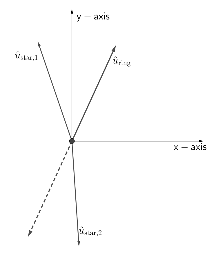
Figure 15: Illustration of the condition for changing the calculation of $\beta$, described in the text.

The angle between the local meridian plane and the detector plane, $\beta$, is also calculated differently for ring spangles compared to planetary spangles. For planetary spangles, the angle is only dependent on their location on the planet. With the detector plane as the reference plane, $\beta$ is calculated as

$$x_{i}y_{i}\geq 0:\ \beta_{i}=\arctan{\frac{y_{i}}{x_{i}}},$$ (20)

$$x_{i}y_{i}<0:\ \beta_{i}=\pi+\arctan{\frac{y_{i}}{x_{i}}},$$ (21)

where the coordinates $(x_{i},y_{i})$ are in the observer reference frame. The addition of $\pi$ is there to make sure the angle that is calculated rotates in the correct direction.

Because all ring spangles have the same normal vector the rotation angle does not depend on the location of the individual spangles. Using the spherical cosine law we can find an equation that instead depends on the orientation of the ring

$$\beta =\arccos{\left(\frac{\cos{\sigma}}{\sin{\theta_{i}}}\right)},$$ (22)

$$\beta =\pi-\arccos{\left(\frac{\cos{\sigma}}{\sin{\theta_{i}}}\right)},\quad\text{if}\quad\hat{u}_{ring}^{y}<0\ ,$$ (23)

with $\sigma=\text{arctan2}\left(\hat{u}_{ring}^{z}/\hat{u}_{ring}^{x}\right)$ the angle the normal vector makes with the $x$-axis and $\hat{u}_{ring}^{z}$ the $z$-component of the normal vector. Again the condition of $\hat{u}^{ring}_{y}<0$ is added to make sure the rotation direction stays the same.