Numerical integrators for confined Langevin dynamics
Abstract
We derive and analyze numerical methods for weak approximation of underdamped (kinetic) Langevin dynamics in bounded domains. First-order methods are based on an Euler-type scheme interlaced with collisions with the boundary. To achieve second order, composition schemes are derived based on decomposition of the generator into collisional drift, impulse, and stochastic momentum evolution. In a deterministic setting, this approach would typically lead to first-order approximation, even in symmetric compositions, but we find that the stochastic method can provide second-order weak approximation with a single gradient evaluation, both at finite times and in the ergodic limit. We provide theoretical and numerical justification for this observation using model problems and compare and contrast the numerical performance of different choices of the ordering of the terms in the splitting scheme.
Keywords: stochastic differential equations with reflection, weak approximation, sampling with constraints, computing ergodic limits, splitting schemes.
AMS Classification: 65C30, 60H35, 60H10, 37H10.
1 Introduction
There is great current demand for reliable numerical methods for solving stochastic differential equations (SDEs). In part this can be attributed to their role in large scale statistical computation, where long stochastic paths are often used to calculate ergodic averages. Many standard algorithms for SDEs are formulated on unbounded domains, e.g. Euclidean space, but in practice are subject to inequality constraints (e.g. positivity relations) or are employed with more complicated domain restrictions, often implemented in an ad hoc manner. In this article, we explore the rational design of numerical algorithms for accurate long-term simulation of Langevin SDEs with domain restriction, including sampling from stationary measures with compact support.
Let be a bounded domain with sufficiently smooth boundary , be the outward normal unit vector at , and be the indicator function of . Let be a positive constant, satisfying certain conditions, and () denote scalar product. Consider the confined Langevin dynamics (CLD) governed by the stochastic differential equations (SDEs):
| (CLD) | ||||
where is a -dimensional standard Wiener process.
The process does not leave the set and it elastically reflects from the boundary [44, 5, 6] which is achieved due to the cádlág process . At the collision of the position with , acts on the momentum to reverse the direction of its component orthogonal to keeping the tangential component unchanged.
If and , i.e., consider the particular case of confined Langevin dynamics (CLD) defined in the set :
| (ECLD) | ||||
where is interpreted as the inverse temperature in molecular dynamics and is a friction parameter. Eq. (ECLD) is ergodic with the invariant density , . The central theme of this paper is the efficient weak-sense numerical approximation of (CLD) including the computation of ergodic limits associated with (ECLD) which is motivated by applications such as those discussed below.
Sampling. Sampling from a desired distribution is of prime importance for computational statistics and it has found a large number of machine learning applications. Many scenarios involve sampling in constrained spaces, for example, truncated data problems arising in survival time studies [23], ordinal data models [21], constrained Lasso and Ridge regression [11], Latent Dirichlet Allocation [2], non-negative matrix factorization [42], and stochastic optimal control [19]. In [27] (see also references therein) the task of sampling from a given distribution with compact support is addressed using reflected Brownian dynamics (in other words, overdamped Langevin dynamics with reflection), where the dynamics are confined within thanks to making use of the local time. In the case of the whole space, advantages of underdamped Langevin equations vs overdamped Langevin dynamics are well studied (see e.g. [26, 14]) which are also expected for the considered confined-space case.
Molecular dynamics. To study molecular properties of a given substance under constant temperature , Langevin dynamics are often employed in which particles (atoms or molecules) with positions move under the action of a potential energy function . These properties can be expressed as ergodic limits associated with Langevin dynamics (see [3, 29, 25] for more details). To perform such simulations in the case of the dynamics being constrained to a confined domain, one typically uses a steep (often singular) barrier in the potential preventing particles from leaving the confined space. The barrier leads to the drift in the Langevin equations increasing rapidly near the boundary of the confined space which can negatively affect stability of numerical methods, or require the use of a variable stepsize [30]. Confined Langevin dynamics (ECLD) serves the purpose of simulating molecular configurations in a restricted region, with atoms undergoing perfectly elastic collisions at the walls, without causing stability problems or requiring stepsize restriction, in contrast to the case of using a steep prohibiting barrier. Furthermore, confined Langevin dynamics offers a natural physical behavior of particles (elastic collisions) at the boundary. In the kinetic theory of gases, for example, specular reflection models are used to describe reflection of gas particles at a totally elastic solid surface [12].
Computational fluid dynamics. The SDEs (CLD) find applications in modelling discrete particles immersed in turbulent flows inside a confined domain, where colloidal particles are carried by the fluid flow, experiencing a drag force and collisions with the domain boundary. Numerical experiments using models of (CLD) type allow to study, e.g., convection, polydispersity etc. related to mesoscopic particles suspended in turbulent flow (see e.g., [15, 32, 10] for more details).
Optimization. Minimizing a loss/error function is at the core of machine learning. In many cases, there are certain constraints which are to be satisfied as a requirement of the model, e.g. positivity constraints. Also, constraining the parameter set can result in improvement of the performance of the model due to regularization effects of constraints, e.g. [43, 28]. One can exploit (ECLD) to minimize a function , where satisfies constraints represented by domain . Moreover, one can also consider replacing with a noisy gradient to introduce batching of data for machine learning specific tasks.
Solving specular boundary value problem. Via the Feynman-Kac formula [6, 7], the SDEs (CLD) provide a probabilistic representation of the specular boundary value problem for linear parabolic partial differential equations (PDEs) (see (2.2)-(2.4)). Solving such PDEs in high dimensions using deterministic methods is computationally infeasible. We can utilise the proposed here numerical methods for (CLD) together with the Monte-Carlo technique to solve such high-dimensional problems.
The above applications give strong motivation to construct and study numerical methods for (CLD). Despite this, very limited attention has been paid so far to numerical integration of confined Langevin dynamics. In this respect we note that in [7] the authors investigated a numerical scheme when and proved its first order weak convergence.
In this paper (Section 3), we derive first-order weak methods to numerically approximate (CLD) as well as second-order schemes in the case of (ECLD). To construct the splitting schemes, we decompose the generator of the Markov process into components representing collisional drift, impulse, and stochastic momentum evolution. In Section 3 we also state theoretical results on error bounds for the methods, both when the SDEs are integrated over a finite time interval and when associated ergodic limits are approximated. Proofs of the error bounds are given in Section 4 with necessary background material for (CLD) and (ECLD) provided in Section 2. The main difficulty in proving convergence arises due to the need to quantify the number of steps with collision. We note the following remarkable fact about second-order symmetric integrators for (ECLD). In a deterministic setting, the discussed splitting approach would typically lead to first-order approximation, even in symmetric compositions [18, 25]. Then stochastic numerics experience [39] suggests that finite-time convergence of a generalization of such deterministic methods to (ECLD) should be of weak order one as well. However, it turns out that the stochastic method with a single gradient evaluation has second-order convergence. Simply put, this counterintuitive and remarkable result is due to the average collision time (within a step of the numerical method in which a collision is encountered) being at the midpoint of the step up to terms of higher order. In Section 5 we present results of numerical tests which confirm our theoretical predictions and compare the methods from Section 3. In Section 6 we summarize this work and suggest topics of interest for further research related to confined Langevin dynamics.
2 Preliminaries
Notation. For the boundary sets we write: and . The space denotes the space of functions whose continuous derivatives exist with respect to , and up to order , and , respectively; has the same meaning but with respect to and ; is a space of functions in with bounded derivatives up to order in and in ; and are functions in with compact support. As usual, denotes the -norm of a vector in . For a differentiable vector-valued function from or to , denotes the Jacobian matrix of evaluated at .
To prove the first-order weak-sense convergence of the schemes proposed in Section 3.1, we need assumptions on the boundary of and the drift coefficient .
Assumption 2.1.
We assume the boundary of set belongs to .
Assumption 2.2.
The coefficient is a function which grows at most linearly in at infinity, i.e. there exists a constant such that,
| (2.1) |
for all and .
In [44], existence of weak solutions and uniqueness in law of (CLD) in with multiplicative noise and , , were established under boundedness assumptions on and the diffusion coefficient . In [5], existence of weak solution of (CLD) in with bounded drift coefficient was shown. This well-posedness result was extended in [6] to the case of being a compact submanifold of , by establishing the existence of a weak solution and its pathwise uniqueness for , and then, by using Girsanov’s theorem, for any bounded . We note that Girsanov’s theorem can be applied if has linear growth in (see [22, Proposition 5.3.6]) as done in [44]. Pathwise uniqueness of the solution of (CLD) with is proved in [47] when is a convex polytope.
2.1 Backward Kolmogorov equation for (CLD)
Consider the backward Kolmogorov equation
| (2.2) |
with terminal condition
| (2.3) |
and specular boundary condition
| (2.4) |
where is the Laplacian with respect to , and are gradients with respect to and , respectively, and .
The solution of (2.2)-(2.4) has the probabilistic representation [6, 7]:
| (2.5) |
where , , solves (CLD) with the starting point .
Below we give three examples of the specular boundary value problem (2.2)-(2.4), for which we can obtain solutions in an explicit form.
Example 2.1.
Take and , , , , and boundary condition at , where . The solution is given by .
Example 2.2.
Let , and . Take , , and boundary condition is . The solution is .
Example 2.3.
Let , , , and . The boundary condition is . Then, the solution is .
Assumption 2.3.
.
Assumption 2.4.
We note that there is a lack of regularity results for solutions of the specular boundary value problem (2.2)-(2.4) available in the literature. The above three examples demonstrate that there is a sufficiently large class of specular boundary value problems whose solutions satisfy Assumption 2.4. Also, it was shown in [7] that if and , then and and exist and belong to .
2.2 Ergodicity
Assumption 2.5.
and for all .
Exploiting the approach used in proving Theorem 3.2 in [34, Section 3] (see also [45]) one can establish under Assumptions 2.1 and 2.5 (note that is bounded thanks to being bounded) that (ECLD) is exponentially ergodic, i.e. there exists a unique invariant measure defined on and the following inequality holds for any , , bounded in and with not faster than polynomial growth in and for any initial point and all :
| (2.6) |
where
Moreover, the invariant measure has a probability density with respect to Lebesgue measure. In [41, Section 9.1.5], geometric ergodicity is proved in the case of the semi-space .
The stationary Fokker-Plank equation for the density has the form
| (2.7) |
with boundary condition
| (2.8) |
As one may check, the Gibbs density
| (2.9) |
indeed satisfies the stationary Fokker-Plank equation (2.7) and the boundary condition (2.8). Here is the normalization constant so that .
In [41, Section 9.1.5], the stationary Fokker-Plank equation (2.7)-(2.8) in the case of was considered. In [6], existence of the solution (in the weak sense) of a McKean-Vlasov Fokker-Plank equation with specular boundary condition was shown.
The above discussion of geometric ergodicity together with numerical methods for (ECLD) introduced in Section 3 equip us with the tools needed to approximately sample from a targeted density , , by choosing , .
To prove error estimates for computing ergodic limits, we need the following assumption on solutions of the backward Kolmogorov equation with specular boundary condition (2.2)-(2.4) related to (ECLD), i.e., of (2.2)-(2.4) with .
Assumption 2.6.
We note that an estimate of the form (2.10) in the case of Langevin equations in the whole space is proved in [45].
Let us discuss the relationship between the confined Langevin dynamics (ECLD) and the reflected gradient SDE (Brownian dynamics with reflection or, in other words, the overdamped reflected Langevin dynamics) [31, 20, 16, 27]:
| (2.11) |
where is the local time of the process on the boundary . The solution of (2.11) belongs to and it is instantaneously reflected along the internal normal to when it hits the boundary . Under the same conditions as we have imposed on the potential and the boundary above, the SDE (2.11) is ergodic with the invariant measure [1], which coincides with , i.e., both (ECLD) and (2.11) can be used for sampling from the Gibbs distribution in the position space. Moreover, analogously to the relationship between Langevin equation and their overdamped limit in the whole space [40] (see also [38, 25]), the solution of (ECLD) tends in distribution to the solution of (2.11) when [13, 44, 32]. In [27] we proposed and studied numerical algorithms for sampling from , , based on (2.11). Benefits of using Langevin equations vs overdamped Langevin dynamics in the case of the whole space are well established (see e.g. [25, 14]). Such a comparison in the case of confined spaces will be investigated in a future work.
3 Numerical methods
In Section 3.1, we present first-order weak methods for the SDEs (CLD). In Section 3.2, we propose splitting schemes for the SDEs (ECLD) which demonstrate (in numerical studies) second-order weak convergence. In Section 3.3, we compare known numerical methods for (CLD) with the schemes of Sections 3.1 and 3.2, and we also discuss multiple collisions. We start this section by describing the ingredients needed for approximating collision dynamics.
Consider a uniform discretization of the time interval with time step , i.e. , , and . We take and .
Approximating , when the position is inside the domain can be done by any suitable standard method of weak approximation of SDEs in the whole space (see e.g. [39, 25]). However, to construct numerical methods for (CLD) and (ECLD), we also need to approximate elastic reflection. Hence the critical part of proposing such methods is to consider steps of a numerical scheme when collisions with happen.
One step with possible collision. Let the current state of a Markov chain approximating the solution of (CLD) be . We construct the next state , of the chain as follows.
If ,
else (i.e., if ) obtained from
The random collision time is found so that if then ensures that the intermediate position (note that ). Thereafter, the numerical method follows the step which results in specular reflection (also known as elastic reflection) of the direction of momentum, and then completes the remaining step in position using the reversed momentum.
If there is more than one solution of , we take the smallest positive value of . Such a choice is possible due to Assumption 2.1 (see [4]). For illustration, consider an annular domain in : and , where and are positive constants such that . Let and , then four possible solutions of are , , and . Here, is negative, so we take .
3.1 First-order schemes
In this section we propose two methods, [PAc] and [AcP]. In the [PAc] scheme the Markov chain first takes an auxiliary step in momentum and then updates position via an Ac step; the order of updates is reversed in [AcP]. We introduce the following notation:
| (3.1) |
where is an -valued random variable such that , , are i.i.d. real-valued random variables with bounded all moments and satisfying
| (3.2) |
The conditions (3.2) are, for instance, satisfied if the are drawn from the standard normal distribution or as i.i.d. discrete random variables with the distribution:
| (3.3) |
In Fig. 3.1 we present the proposed schemes. For the sake of clarity, we describe [PAc] scheme in detail. As already mentioned, the aim is to construct a Markov chain to approximate (CLD) in the weak sense. At every iteration moving from to , the Markov chain first takes auxiliary steps in velocity and in position, denoted by and respectively:
| (3.4) |
where and they are mutually independent. The next state of the Markov chain, and , is evaluated according to Ac(, , which means that if , then and , else and , where .
| [PAc] | ||
| [AcP] | ||
Schemes [PAc] and [AcP] have finite-time convergence with first weak order when they are applied to (CLD). By way of illustration, we state below Theorem 3.1 for scheme [PAc] which is proved in Section 4.1. When these schemes are applied to the ergodic SDE (ECLD), they approximate the ergodic limit with error . We state below the corresponding Theorem 3.2 for scheme [PAc] which is proved in Section 4.2.
Theorem 3.1.
3.2 [Ac, B, O] splitting schemes
In the whole space (i.e., without a reflective boundary) splitting schemes of second weak order for the Langevin equations, which rely on a concatenation of the exact integration for the drift and impulse and of the Ornstein-Uhlenbeck process at each time step, are known for their excellent performance in molecular dynamics and statistics applications (see, e.g. [35, 9, 24, 25, 39] and references therein). Hence, it is natural to extend those methods to the confined Langevin dynamics (ECLD). The [Ac, B, O] splitting schemes proposed in this subsection degenerate to the standard deterministic Störmer-Verlet schemes with collision step Ac when (ECLD) degenerates to the (deterministic) Hamiltonian system with elastic collisions. Such deterministic schemes have been shown to be first order accurate due to the collision step Ac having local error of order [18, 25]. Because of this, stochastic numerics experience [39] suggests that finite-time weak convergence of the [Ac, B, O] schemes for (ECLD) should be first order, too. However, the [Ac, B, O] schemes for (ECLD) unexpectedly turned out to be of weak order , which we demonstrate in several carefully constructed and performed numerical experiments (Section 5) and theoretically justify when is a half-space, i.e. , in Section 4.3.
Let be an valued random variable such that , , are i.i.d. real-valued random variables with bounded all moments and satisfying
| (3.7) |
The conditions (3.2) are, for instance, satisfied for having the standard normal distribution or being i.i.d. discrete random variables with the distribution:
| (3.8) |
In Fig. 3.2, and and they all are mutually independent. Introduce the notation
The three proposed methods are presented in Fig. 3.2. It is straightforward to write down the other three possible symmetric concatenations, namely [BOAcOB], [AcBOBAc], [AcOBOAc], which we test in Experiment 5.2.
| [OBAcBO] | ||
| [BAcOAcB] | ||
| [OAcBAcO] | ||
3.3 Comparison with other numerical integrators for (CLD)
Here we present a comparison of previously known schemes for (CLD) with the numerical integrators proposed in the previous two subsections.
Let . In [7] (see also [8, 32]), the authors studied a symmetrized scheme in which, given at time , the approximate position is always updated as
| (3.9) |
At every step, is calculated. A collision happens if . In that case
If no collision occurs then (i.e., the straightforward Euler update). This scheme was generalized to half-space in higher dimensions, i.e. , in [8, 7, 32].
The main difference between the above scheme and our schemes lies in the update of momentum. In the scheme above, it is possible for the momentum to get reversed already in the interval due to a realized large Wiener increment. In such a case the update results in a direction towards the negative axis, which leads to multiple collisions during the time interval . However, this pathological situation does not arise, by construction, in the schemes [AcP], [PAc] and the splitting schemes of Section 3.2 if implemented for . We also observe that if one extends the symmetrized reflection of (3.9) around the boundary in curved domains, then the symmetrized reflection around the boundary along the normal does not imitate specular reflection of (CLD), unlike the schemes of Sections 3.1 and 3.2.
Further, some penalized schemes for (CLD) are also proposed in [32] without analysis. It is known (see [4, 39, 27] and references therein) that symmetrized reflection and penalized schemes are good candidates to approximate the reflected SDEs (2.11), in which the local time is responsible for keeping the trajectories in . In contrast, the confinement of position in is achieved in (CLD) by the cádlág process whose explicit expression is known via values of . In comparison with the existing schemes, all our schemes are constructed utilizing the expression for , which, in particular, ensures conservation of (conjugate) momenta in the event of collision, i.e.,
| (3.10) |
where . Since the collision is interlaced in the one-step procedure of the discrete dynamics, estimates related to the average number of collisions become crucial for the global error analysis (see Lemmas 4.3 and 4.6).
Although we present our results in a bounded domain with boundary , the results can be extended to the half-space or any other unbounded domain with boundary satisfying Assumption 2.1. The only additional requirement is moment bounds for (moments of are typically bounded for most forces and potentials of interest), which can be obtained under a global Lipschitz assumption on or replaced by using the concept of rejecting trajectories [36, 39] in the non-globally Lipschitz case. Furthermore, the proposed schemes can be justified in the case of convex domains with piecewise boundary, too.
In our schemes, multi-collisions in a single time-step can occur for a curved bounded domain when is large and/or (see Ac step) is small, i.e. when with sufficiently large speed, the particle collides with the curved wall in the grazing manner. In this case calculated in Ac will not lie in . We note that when is a convex polytope, we can always choose sufficiently small such that multi-collisions occur with exponentially low probability as in this case multi-collisions can only happen when is very large. It is also clear that there is no possibility in our schemes for multi-collisions in half-space. But when is curved, geometry comes into the picture and it may potentially result in multi-collisions in the discrete dynamics. Obviously, our schemes can be adapted to this situation by applying the Ac step recursively. The question that remains to be answered is how many times we need to utilize this recursion. Let us again consider the one-step procedure of [PAc] scheme: depending on the update of the momentum P, Ac is deterministic which means the dynamics becomes billiard-like in high dimensions, i.e., a straight line motion between two collisions.
For the sake of the discussion here, let us denote by the position and new velocity, respectively, after the P step in [PAc]. Also, denote the continuous-time dynamics evolving according to the Ac step by . As already highlighted, the dynamics of follows straight paths, and indeed is the exact solution of the following ODE system:
in the interval . It is clear that the dynamics in the duration of may have multiple collisions. It is proved in [33, p. 5], that the Lebesgue measure of a set of configurations for which one encounters infinite collisions in finite time (in the above case in time from to ) and for which dynamics hit the boundary with zero normal component of velocity is zero. Hence, we expect that the number of trajectories corresponding to our schemes which experience multiple collisions in a single step are negligible for sufficiently small and, indeed, this was confirmed in our experiments (see Section 5).
We observe that all the schemes of Sections 3.1 and 3.2 can be implemented to account for more than one collision in a step. In practice, for simplicity, we suggest to reject trajectories for which more than one collision occurs in a step of the Markov chain. In experiments for the ergodic case (i.e., during long time simulations) on a circular domain of radius two in two dimensions, we encountered multiple collisions in less than out of simulated trajectories for , and we observed no steps with multiple collisions for , i.e. the effect of multiple collisions in our schemes is negligible, as expected. Similar results were seen in the case where we chose to deliberately push the dynamics towards the boundary to enhance the number of collisions (see Experiment 5.4).
4 Proofs
In this section, for the first-order scheme, we prove the finite-time convergence Theorem 3.1 (Section 4.1) and Theorem 3.2 (Section 4.2) on the error estimate for computing ergodic limits. We also provide a justification (Section 4.3) for second-order weak convergence of the splitting schemes from Section 3.2.
4.1 Proof of Theorem 3.1
The proof is based on two main ingredients: a one-step error estimate (Lemma 4.2) and an estimate related to the average number of collisions (Lemma 4.3). According to the lemmas, inside the domain, where we use the usual Euler-type walker, the one-step error is and the walker makes steps; the error in the collision steps is but the average number of collision steps is bounded and independent of the time step . The finite-time error is naturally . We note that the position in the continuous dynamics (CLD) and its discrete approximation is bounded as we consider (CLD) in a bounded domain . At the same time, momentum lives in and hence, to prove convergence, we need that moments of its discrete approximation are bounded (see Lemma 4.1). The proof relies on the fact that the drift in (CLD) is growing at most linearly in and the noise is additive.
Lemma 4.1.
Proof.
Next we estimate the one-step weak error.
Lemma 4.2.
Proof.
In the proof the letter is used for positive constants and for positive integers which can change from line to line. We note that it follows from (4.2) that
where is independent of , , .
We have
| (4.3) | ||||
Consider the first term. Using Taylor’s expansion and Assumption 2.4, we obtain
where the remainder satisfies
with being a constant independent of , , .
Using Taylor’s expansion again for around and around , we get for the second term in (4.3):
where we have used and from (2.4). Here , , satisfy
| (4.4) |
with being a constant independent of , , . Now, applying Taylor’s formula to around and around , we obtain
where is the Jacobian of with respect to evaluated at with
| (4.5) |
and satisfies (4.4).
Combining the obtained expressions for and , we ascertain that
with satisfying
| (4.6) |
with being a constant independent of , , . Taking the expectation conditioned on , we get
| (4.7) |
where we have expanded around and then around , and satisfies
| (4.8) |
with being a constant independent of , , .
With the usual Taylor expansion calculation for the Euler scheme for SDEs (see e.g. [39, Chap. 7]), we can write
| (4.9) |
where satisfies (4.8).
∎
The estimate in the above local error lemma contains the term of order corresponding to the error of approximating collisions. Consequently, the next lemma, related to the average number of collisions when the Markov chain encounters the boundary , plays a major role in global convergence analysis of the considered first-order methods. Its proof rests on the boundary value problem associated with the Markov chain :
| (4.10) | |||||
| (4.11) |
where is the one-step transition operator:
and . The solution to this problem is given by [46, 37, 39]:
| (4.12) |
Lemma 4.3.
Proof.
If we can find a function with , satisfying (4.10)-(4.11), such that
| (4.14) |
then the inequality, will hold. Therefore, the aim is to construct a function satisfying (4.14).
Consider a boundary zone defined as . Due to [4, Proposition 1], there is an such that the projection of on is unique whenever . Introduce the function
where is an valued function such that when ; here is the projection of on . Note that due to Assumption 2.1 (see [4, Proposition 1]). We extend the function from to so that and , where is the Hölder norm and depends on . Such an extension is possible due to [17, Lemma 6.37]. We choose the constant so that is always positive. Note that is a bounded function (with bounded derivatives up to third order), hence it is possible to make such a choice of . The choice of the constant will be discussed later in the proof.
The proof of Lemma 4.1 implies for any
| (4.15) |
and
| (4.16) |
where and satisfy for any :
and
with being independent of and .
Given , we now aim at calculating . Using Taylor’s theorem, we obtain
| (4.17) |
and
| (4.18) |
where , , and denotes the Jacobian matrix of evaluated at . Therefore, we get
| (4.19) |
Since and using (4.18), we obtain
| (4.20) |
Due to the boundedness of first derivatives of , we ascertain
where is a generic constant independent of . Using these estimates, (4.20) becomes
| (4.21) |
where with being independent of and . Using (4.15) and linear growth of in , we obtain
| (4.22) |
where with being independent of and . Using (4.15) and (4.16), we get
| (4.23) |
where with being independent of and . From (4.22) and (4.23), we have
| (4.24) |
where with being independent of and .
Using (4.16) with , we have
| (4.25) |
where and with independent of , and . Recall that , where is independent of , and . Therefore, using (4.24) and (4.25), we get
| (4.26) |
Hence, there are sufficiently large and sufficiently small so that . This proves that (4.13) holds with a constant independent of (it depends on and ).
∎
4.2 Proof of Theorem 3.2
The proof of Theorem 3.2 has the same ingredients as the proof of Theorem 3.1 in the previous section with the major difference that the global error bound in Theorem 3.2 should not depend on the integration time since here we are interested in ergodic limits associated with (ECLD), while the error bound in Theorem 3.1 for the approximation of (CLD) on the finite time interval can depend on . We start (Lemma 4.4) by estimating moments of the momentum uniformly in . Next, in Lemma 4.5, we consider the one-step (local) error. An estimate related to the average number of collisions of the Markov chain with the boundary is obtained in Lemma 4.6.
Lemma 4.4.
Proof.
The constant is changing from line to line. Using (3.10), we get (see the proof of Lemma 4.1):
where depends on only. It is not difficult to obtain
with independent of (it depends on and moments of . Using the generalized Young’s inequality, i.e. ; , ; ; , with , , , and , we get
In the similar manner, we have
and similarly with some new
Next note that
and, using the Gronwall lemma, we get
∎
Lemma 4.5.
The proof follows exactly the same steps as in the proof of Lemma 4.2 with the modification that Assumption 2.6 is used for derivatives’ decay to bound the terms in the Taylor expansion.
Lemma 4.6.
Proof.
If in (4.10) then the solution of (4.10)-(4.11) is
If we can find a function with , satisfying (4.10)-(4.11), such that
then the inequality holds.
As in the proof of Lemma 4.3, we consider the boundary zone . Introduce the function
where ; integer will be chosen later in the proof; is a constant, which value will also be chosen later in the proof; and is the same as in the proof of Lemma 4.3 (i.e., for and is projection of on ). Note that .
Using Taylor’s expansion, we get for any
where satisfies
| (4.29) |
with being independent of and . Expanding , using the generalised Young inequality twice and then simplifying the expression, we obtain
| (4.30) | |||
where satisfies (4.29) with .
Applying similar arguments used to obtain (4.24), we get
| (4.31) |
where satisfies
| (4.32) |
with being independent of and (it depends on .
From (4.30) and (4.31) and using it follows that
where satisfies (4.32). Choosing a sufficiently large and, depending on the choice of choosing a sufficiently small and large , we get . Hence, the lemma is proved.
∎
4.3 One-step lemma for scheme [OBAcBO]
Consider In this case the one step of scheme [OBAcBO] from Section 3.2 takes the form:
Here the components of and of are i.i.d. with the standard normal distribution and , , denotes th component of and likewise for and , .
In this section we need the following assumptions. The potential satisfies Assumption 2.5, and is globally Lipschitz and derivatives of are bounded. To ensure ergodicity (see [34] and [41][Section 9.1.5]), we need dissipativity of the extended generator of the Markov process which can be guaranteed by assuming that there exists an and such that
| (4.33) |
Further, we assume that the function and all its existing derivatives have growth at most polynomially in and . As usual for proofs of higher order numerical methods, we also require that the solution of the backward Kolmogorov equation (2.2)-(2.4) with is sufficiently smooth and, in particular, satisfies the condition that there are positive constants and independent of such that the following bound holds for some (cf. (2.10) in Assumption 2.6):
where is independent of and .
By standard means it is not difficult to establish that under the stated conditions the moments of and from scheme [OBAcBO] are bounded uniformly in time (cf. Lemma 4.4).
Lemma 4.7.
Assume that the above conditions hold and that is random with a density so that all the required moments with respect to this density exist, then the one-step error of scheme [OBAcBO] has the following estimate
| (4.34) |
where is independent of and .
Discussion The number of steps is while we expect (cf. Lemmas 4.3 and 4.6) that the average number of steps with collisions is independent of . This together with (4.34) leads to the claim that [OBAcBO] (and analogously other schemes of Section 3.2) has second weak convergence order in , both at finite time and for the ergodic limit. We recall again that the deterministic counterpart of [OBAcBO] has first order convergence and second order is achieved here thanks to an average (see details in the proof of this lemma) of the collision time being equal to up to terms of order .
Proof.
We write the one step error as
Appropriately applying Taylor’s expansion to each of the brackets in the above re-writing of , we arrive at
where and . Introduce so that i.e., We have
where satisfies the same estimate as above.
Let us first consider the following component of (4.3). Using the expression for we get
where
Let be the joint density for Assume that all the required moments with respect to this density exist. We have
Note that
Hence
Next consider the following component of (4.3):
Thus . The terms for
are analyzed analogously. ∎
5 Numerical tests
In this section we confirm theoretical results for the numerical integrators from Section 3 in both the finite-time and ergodic case.
The following notation is used in this section. The Monte Carlo estimator for is , where are independent realizations of ; denotes the number of collisions along a trajectory and is the Monte-Carlo estimator for the average number of collisions; and denotes the usual sample variance of Monte Carlo estimators.
Experiment 5.1.
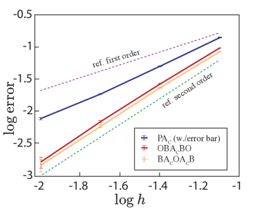
In this experiment we consider finite-time weak convergence. Consider Example 2.2 with and , , and the final time . Hence, the solution is . The point at which is evaluated in the experiments is and . To compute the global error , we calculate the exact solution (5 d.p.). We test the first-order scheme [PAc] and two second-order schemes [OBAcBO] and [BAcOAcB]. Tables 5.2 and 5.3 and Fig. 5.1 confirm second-order accuracy of [OBAcBO] and [BAcOAcB]. The first-order method [PAc] had slightly higher accuracy than first order but clearly lower than second order. In this experiment step in [OBAcBO] and [BAcOAcB] schemes is
| 0.08 | 0.139994 | ||||
|---|---|---|---|---|---|
| 0.04 | |||||
| 0.02 | 0.018207 | ||||
| 0.01 | 0.007568 |
| 0.08 | 0.095775 | ||||
|---|---|---|---|---|---|
| 0.04 | |||||
| 0.02 | 0.006776 | ||||
| 0.01 | 0.001591 |
| 0.08 | 0.083880 | ||||
|---|---|---|---|---|---|
| 0.04 | |||||
| 0.02 | 0.005807 | ||||
| 0.01 | 0.001431 |
| [AcBOBAc] | [AcOBOAc] | ||
|---|---|---|---|
| 0.5 | |||
| 0.4 | |||
| 0.2 | |||
| 0.1 | |||
| 0.08 |
| [BAcOAcB] | [BOAcOB] | |||
|---|---|---|---|---|
| 0.5 | ||||
| 0.4 | ||||
| 0.2 | ||||
| 0.1 | ||||
| 0.08 |
| [OAcBAcO] | [OBAcBO] | |||
|---|---|---|---|---|
| 0.5 | ||||
| 0.4 | ||||
| 0.2 | ||||
| 0.1 | ||||
| 0.08 |
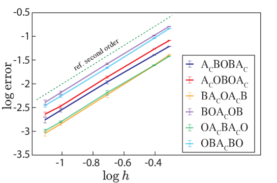
Experiment 5.2.
In this experiment we test convergence of second-order integators [AcBOBAc], [AcOBOAc], [BAcOAcB], [BOAcOB], [OAcBAcO] and [OBAcBO] to ergodic limits.
Take and . Consider (ECLD) with the potential
and , . For numerical simulation, we choose as a sufficiently large time to achieve accurate values of the ergodic limit of with respect to this choice of (ECLD). The exact value of is (4 d.p.). The starting point of Markov chain is and . We denote . The results are presented in Tables 5.4-5.6 and Fig. 5.2, which clearly show second order convergence for all the integrators. As expected [24, 25], [BAcOAcB] and [OAcBAcO] are the most accurate schemes.
| 0.1 | ||
|---|---|---|
| 0.075 | ||
| 0.05 | ||
| 0.04 |
| 0.1 | ||
|---|---|---|
| 0.075 | ||
| 0.05 | ||
| 0.04 |
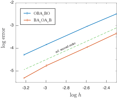
Experiment 5.3.
In this experiment we test convergence of second-order integators [BAcOAcB] and [OBAcBO] to ergodic limits. Take G:= . Consider (ECLD) with the potential
and , . We choose
We note that the potential is not symmetric around zero and that its local minima lie outside . We are interested in approximating . We take . We calculate the integral using integral2 function in Matlab with tolerance which gives the reference value (5 d.p.). The starting point of the Markov chain is with . We denote . The results are presented in Tables 5.7-5.8 and Fig. 5.3, which clearly show second-order convergence for both integrators with [BAcOAcB] being more accurate.
| 0.25 | 2.102 | |||
| 0.2 | 1.888 | |||
| 0.1 | 0.940 | |||
| 0.08 | ||||
| 0.05 | 0.3486 | |||
| 0.04 | 0.2431 | |||
| 0.025 | 0.1141 | |||
| 0.02 | 0.0762 | |||
| 0.01 | 0.0215 | |||
| 0.008 | 0.01450 | |||
| 0.004 | 0.003670 | |||
| 0.002 | 0.000928 |
| 0.25 | 2.088 | |||
| 0.2 | 1.855 | |||
| 0.1 | 0.932 | |||
| 0.08 | 0.676 | |||
| 0.05 | 0.331 | |||
| 0.04 | 0.2310 | |||
| 0.025 | 0.1141 | |||
| 0.02 | 0.0708 | |||
| 0.01 | 0.0202 | |||
| 0.008 | 0.01337 | |||
| 0.004 | 0.00356 | |||
| 0.002 | 0.00090 |
| [BAcOAcB] | [OBAcBO] | ||
|---|---|---|---|
| 0.25 | |||
| 0.3 | |||
| 0.35 | |||
| 0.42 | |||
| 0.5 |
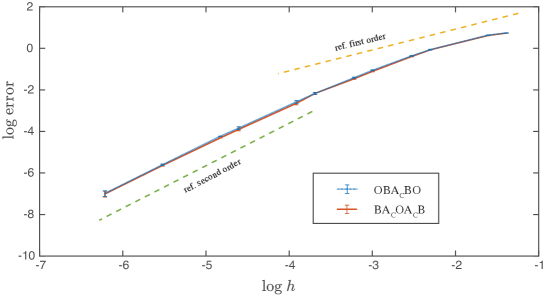
Experiment 5.4.
We take and . We sample from distribution given by
| (5.1) |
and compute
| (5.2) |
via its Monte Carlo estimator based on two schemes [OBAcBO] and [BAcOAcB] which are used to discretize (ECLD). We take in order to increase the number of collisions with the boundary and the aim is to check if in this case the two schemes [OBAcBO] and [BAcOAcB] maintain second order of convergence asymptotically as the discretization step decreases. We take the initial conditions and .
We divide our analysis in two parts, in the first we are interested in this experiment to investigate the asymptotic convergence of [OBAcBO] and [BAcOAcB] as becomes smaller. Here it is crucial as our choice of results in large number of collisions in time period from to . It is clear from Tables 5.9 - 5.10 and Fig. 5.4 that both numerical schemes [OBAcBO] and [BAcOAcB] have convergence then convergence and, as decreases, we clearly observe convergence. In the second part, we study the large step size regime and investigate which of the methods is more stable. It is clear from Table 5.11 that [BAcOAcB] is more stable than [OBAcBO]; it allows the use of step sizes of around 0.42, whereas [OBAcBO] becomes unstable for a step size greater than about 0.30.
6 Conclusions
We constructed and analysed a number of numerical methods for simulating confined Langevin dynamics. The considered SDE model can be used in a variety of applications from molecular dynamics to sampling from distributions with compact support and optimization with constraints. We proved finite-time convergence and convergence to ergodic limits for our first-order schemes. We observed and justified (in the case of half-space) a surprising result that the proposed [Ac, B, O] Störmer-Verlet-type splitting schemes are of second weak order despite their deterministic counterparties are only of first order due to the collision step Ac having local error of order .
A number of extensions for this work are of interest. Those include further testing of the proposed geometric integrators, e.g. applying them to train neural networks with imposed constraints on weights. It is possible to extend the developed approach to the case when particles are not only colliding with the boundary of a domain but also with each other. Constructing efficient numerical methods for Langevin equations with non-elastic collisions on boundary is a possible topic for future work. Further theoretical analysis of the constructed second-order integrators deserves a separate attention too.
Acknowledgments
AS and MVT were supported by the Engineering and Physical Sciences Research Council [grant number EP/X022617/1]. The authors express their gratitude to the International Centre for Mathematical Sciences (ICMS) for its support via the research-in-groups scheme. For the purpose of open access, the authors have applied a CC BY public copyright licence to any Author Accepted Manuscript version arising.
References
- [1] A. Benchérif-Madani and É. Pardoux. A probabilistic formula for a Poisson equation with Neumann boundary condition. Stoch. Anal. Appl., 27(4):739–746, 2009.
- [2] D. M. Blei, A. Y. Ng, and M. I. Jordan. Latent Dirichlet allocation. J. Mach. Learn. Res., 3:993–1022, 2003.
- [3] S. D. Bond and B. Leimkuhler. Molecular dynamics and the accuracy of numerically computed averages. Acta Numerica, 16:1, 2007.
- [4] M. Bossy, E. Gobet, and D. Talay. A symmetrized Euler scheme for an efficient approximation of reflected diffusions. J. Appl. Prob., 41(3):877–889, 2004.
- [5] M. Bossy and J.-F. Jabir. On confined McKean Langevin processes satisfying the mean no-permeability boundary condition. Stoch. Proc. Applic., 121(12):2751 – 2775, 2011.
- [6] M. Bossy and J.-F. Jabir. Lagrangian stochastic models with specular boundary condition. J. Funct. Anal., 268(6):1309 – 1381, 2015.
- [7] M. Bossy, J.-F. Jabir, and R. Maftei. Convergence rate analysis of time discretization scheme for confined Lagrangian processes. ⟨hal-01656716⟩, 2017.
- [8] M. Bossy, R. Maftei, J.-P. Minier, and C. Profeta. A stochastic approach to colloidal particle collision/agglomeration. arXiv:1611.06248, 2016.
- [9] N. Bou-Rabee and H. Owhadi. Long-run accuracy of variational integrators in the stochastic context. SIAM J. Numer. Anal., 48(1):278–297, 2010.
- [10] L. Campana, M. Bossy, and C. Henry. Lagrangian stochastic model for the orientation of inertialess spheroidal particles in turbulent flows: An efficient numerical method for CFD approach. Computers and Fluids, 257:105870, 2023.
- [11] G. Celeux, M. El Anbari, J.-M. Marin, and C. P. Robert. Regularization in regression: Comparing Bayesian and frequentist methods in a poorly informative situation. Bayesian Anal., 7(2):477–502, 06 2012.
- [12] C. Cercignani. The Boltzmann equation and its applications. Springer, 1988.
- [13] C. Costantini. Diffusion approximation for a class of transport processes with physical reflection boundary conditions. Ann. Prob., 19(3):1071–1101, 1991.
- [14] R. L. Davidchack, T. E. Ouldridge, and M. V. Tretyakov. New Langevin and gradient thermostats for rigid body dynamics. J. Chem. Phys., 142(14):144114, 2015.
- [15] M. Ebrahimian, R. S. Sanders, and S. Ghaemi. Dynamics and wall collision of inertial particles in a solid–liquid turbulent channel flow. J. Fluid Mech., 881:872–905, 2019.
- [16] M. Freidlin. Functional integration and partial differential equations. Princeton Univ. Press, 1985.
- [17] D. Gilbarg and N.S. Trudinger. Elliptic partial differential equations of second order. Springer, 1983.
- [18] Y. A. Houndonougbo, B. B. Laird, and B. Leimkuhler. A molecular dynamics algorithm for mixed hard-core/continuous potentials. Molecular Physics, 98(5):309–316, 2000.
- [19] V. A. Huynh, S. Karaman, and E. Frazzoli. An incremental sampling-based algorithm for stochastic optimal control. Intern. J. Robotics Res., 35(4):305–333, 2016.
- [20] N. Ikeda and S. Watanabe. Stochastic differential equations and diffusion processes. North-Holland, 1989.
- [21] V.E. Johnson and J.H. Albert. Ordinal data modeling. Springer, 2006.
- [22] I. Karatzas and S.E. Shreve. Brownian motion and stochastic calculus. Springer, 1991.
- [23] J.P. Klein and M.L. Moeschberger. Survival analysis: techniques for censored and truncated data. Springer, 2005.
- [24] B. Leimkuhler and C. Matthews. Rational construction of stochastic numerical methods for molecular sampling. Appl. Math. Res. Express, 2013(1):34–56, 2013.
- [25] B. Leimkuhler and C. Matthews. Molecular dynamics with deterministic and stochastic numerical methods. Springer, 2015.
- [26] B. Leimkuhler, C. Matthews, and G. Stoltz. The computation of averages from equilibrium and nonequilibrium Langevin molecular dynamics. IMA J. Num. Anal., 36:13–79, 2016.
- [27] B. Leimkuhler, A. Sharma, and M. V. Tretyakov. Simplest random walk for approximating Robin boundary value problems and ergodic limits of reflected diffusions. Ann. Appl. Prob., 33(3):1904–1960, 2023.
- [28] B. Leimkuhler, T. J. Vlaar, T. Pouchon, and A. Storkey. Better training using weight-constrained stochastic dynamics. In Marina Meila and Tong Zhang, editors, Proceedings of the 38th International Conference on Machine Learning, volume 139, pages 6200–6211. PMLR, 2021.
- [29] T. Lelièvre, M. Rousset, and G. Stoltz. Free energy computations: A mathematical perspective. Imperial College Press, 2010.
- [30] A. Leroy, B. Leimkuhler, J. Latz, and D. Higham. Adaptive stepsize algorithms for Langevin dynamics. arXiv:2403.11993, 2024.
- [31] P.L. Lions and A.S. Sznitman. Stochastic differential equations with reflecting boundary conditions. Comm. Pure Appl. Math., 37(4):511–537, 1984.
- [32] R. Maftei. Stochastic analysis for Lagrangian particles simulation : application to colloidal particle collision. Theses, Université Côte d’Azur, December 2017.
- [33] C. Marchioro, A. Pellegrinotti, E. Presutti, and M. Pulvirenti. On the dynamics of particles in a bounded region: A measure theoretical approach. J. Math. Phys., 17(5):647–652, 08 1976.
- [34] J.C. Mattingly, A.M. Stuart, and D.J. Higham. Ergodicity for SDEs and approximations: locally Lipschitz vector fields and degenerate noise. Stoch. Proc. Applic., 101(2):185 – 232, 2002.
- [35] G. N. Milstein and M. V. Tretyakov. Numerical methods for Langevin type equations based on symplectic integrators. IMA J. Numer. Anal., 23:593–626, 2003.
- [36] G. N. Milstein and M. V. Tretyakov. Numerical integration of stochastic differential equations with nonglobally Lipschitz coefficients. SIAM J. Numer. Anal., 43(3):1139–1154, 2005.
- [37] G.N. Milstein and M.V. Tretyakov. Simulation of a space-time bounded diffusion. Ann. Appl. Probab., 9(3):732–779, 1999.
- [38] G.N. Milstein and M.V. Tretyakov. Computing ergodic limits for Langevin equations. Physica D, 229(1):81 – 95, 2007.
- [39] G.N. Milstein and M.V. Tretyakov. Stochastic numerics for mathematical physics. Springer, 2nd edition, 2021.
- [40] E. Nelson. Dynamical theories of Brownian motion. Princeton Univ. Press, 1967.
- [41] F. Nier. Boundary conditions and subelliptic estimates for geometric Kramers-Fokker-Planck operators on manifolds with boundaries. Memoirs AMS, 252, 2013.
- [42] J. W. Paisley, D. Blei, and M. I. Jordan. Bayesian nonnegative matrix factorization with stochastic variational inference. In Handbook of mixed membership models and their applications, 2014.
- [43] S. Sangalli, E. Erdil, A. Hoetker, O. F. Donati, and E. Konukoglu. Constrained optimization to train neural networks on critical and under-represented classes. In NeurIPS, 2021.
- [44] K. Spiliopoulos. A note on the Smoluchowski-Kramers approximation for the Langevin equation with reflection. Stochastics and Dynamics, 07(02):141–152, 2007.
- [45] D. Talay. Stochastic Hamiltonian systems: exponential convergence to the invariant measure, and discretization by the implicit Euler scheme. Markov Proc. Relat. Fields, 8:163–198, 2002.
- [46] A.D. Wentzell. A course in the theory of stochastic processes. McGraw-Hill, 1981.
- [47] T. Önskog. Existence of pathwise unique Langevin processes on polytopes with perfect reflection at the boundary. Stat. & Probab. Lett., 83(10):2211–2219, 2013.