Fast Machine-Precision Spectral Likelihoods for Stationary Time Series

Abstract

We provide in this work an algorithm for approximating a very broad class of symmetric Toeplitz matrices to machine precision in $\mathcal{O}(n\log n)$ time. In particular, for a Toeplitz matrix $\bm{\Sigma}$ with values $\bm{\Sigma}_{j,k}=h_{\left|j-k\right|}=\int_{-1/2}^{1/2}e^{2\pi i\left|j-k\right|\omega}S(\omega)\mathop{}\!\mathrm{d}\omega$ where $S(\omega)$ is piecewise smooth, we give an approximation $\mathbb{\mathcal{F}}\bm{\Sigma}\mathbb{\mathcal{F}}^{H}\approx\bm{D}+\bm{U}\bm{V}^{H}$, where $\mathbb{\mathcal{F}}$ is the DFT matrix, $\bm{D}$ is diagonal, and the matrices $\bm{U}$ and $\bm{V}$ are in $\mathcal{C}^{n\times r}$ with $r\ll n$. Studying these matrices in the context of time series, we offer a theoretical explanation of this structure and connect it to existing spectral-domain approximation frameworks. We then give a complete discussion of the numerical method for assembling the approximation and demonstrate its efficiency for improving Whittle-type likelihood approximations, including dramatic examples where a correction of rank $r=2$ to the standard Whittle approximation increases the accuracy from $3$ to $14$ digits for a matrix $\bm{\Sigma}\in\mathbb{R}^{10^{5}\times 10^{5}}$. The method and analysis of this work applies well beyond time series analysis, providing an algorithm for extremely accurate direct solves with a wide variety of symmetric Toeplitz matrices. The analysis employed here largely depends on asymptotic expansions of oscillatory integrals, and also provides a new perspective on when existing spectral-domain approximation methods for Gaussian log-likelihoods can be particularly problematic.

1 Introduction

Let $\bm{\Sigma}\in\mathbb{R}^{n\times n}$ be a symmetric Toeplitz matrix with entries $\bm{\Sigma}_{j,k}=h_{\left|j-k\right|}=\int_{-1/2}^{1/2}e^{2\pi i\omega\left|j-k\right|}S(\omega)\mathop{}\!\mathrm{d}\omega$. In this work we discuss approximations $\mathbb{\mathcal{F}}\bm{\Sigma}\mathbb{\mathcal{F}}^{H}\approx\bm{D}+\bm{U}\bm{V}^{H}$ where $\bm{D}$ is diagonal, $\bm{U},\bm{V}\in\mathbb{C}^{n\times r}$ form a matrix of rank $r\ll n$, and $\mathbb{\mathcal{F}}$ is the discrete Fourier transform (DFT) matrix, parameterized in the unitary form with the “fftshift” for convenience as $\mathbb{\mathcal{F}}=[n^{-1/2}e^{-2\pi ijk/n}]_{j\in(-n/2):(n/2-1),k\in 0:(n-1)}$. These matrices are of fundamenal importance in time series analysis, and several motivating aspects of the derivation will be done in that language. But while time series analysis provides a convenient and elegant way to study the problem, all of the tools discussed and applied below are applicable to any symmetric Topelitz matrix whose “generating” function $S(\omega)$ (called a spectral density in the time series literature when $S(\omega)\geq 0$ and $S(\omega)=S(-\omega)$) is known and meets some basic requirements like being piecewise smooth. As will be demonstrated, however, the method still applies when the function $S(\omega)$ takes negative values, and so this structure can potentially be exploited for a wide variety of symmetric Toeplitz matrices and applications beyond just time series analysis.

To establish statistical notation and introduce relevant concepts for the remainder of this work, consider the length-$n$ mean-zero time series $\left\{Y_{t}\right\}_{t=0}^{n-1}$. If $\left\{Y_{t}\right\}$ is stationary, which we will assume it is for the duration of this work, then it has an autocovariance sequence given by $h_{k}=\text{Cov}(Y_{t+k},Y_{t})$ for any $t$. The Cramér spectral representation theorem [7] states that there exists an orthogonal increment process $Z(\nu)$ defined on $(-1/2,1/2]$ such that

$$Y_{t}=\int_{(-1/2,1/2]}e^{2\pi it\nu}dZ(\nu).$$

Corresponding to $Z$ there is a spectral distribution function $F$ such that $F(\tau)=0$ for $\tau\leq-1/2$, $F(\tau)=h_{0}$ for $\tau\geq 1/2$, and $F(\mu)-F(\tau)=\text{Var}(Z(\mu)-Z(\tau))$ for $-1/2<\tau<=\mu<1/2$ [7]. Herglotz’s theorem gives that

$$h_{k}=\int_{(-1/2,1/2]}e^{2\pi ik\nu}dF(\nu),$$

and if $F$ has a density with respect to the Lebesgue measure, which we will denote $S$, that density is called the spectral density. A basic fact about covariance functions is that they must be positive (semi-)definite, and that spectral densities, when they exist, must be non-negative (and symmetric about the origin for real-valued processes). In light of this fact, it is clearly easier to specify a parametric family of valid spectral densities than it is a family of valid covariance functions. Unsurprisingly, then, in many settings modeling dependence structure in the spectral domain is an appealing choice for practitioners.

A second reason that makes modeling covariance structure in the spectral domain appealing is that the DFT of the vector $\bm{y}$ (with $\bm{y}_{j}=Y_{j}$) often has a better-behaved covariance matrix than $\bm{y}$ itself does. If $\left\{Y_{t}\right\}$ is measured with no gaps and a constant sampling rate (which will be assumed to be unit sampling for the duration of this work without loss of generality), the covariance matrix of $\bm{y}$, denoted $\bm{\Sigma}$ with $\bm{\Sigma}_{j,k}=h_{|j-k|}$, is Toeplitz, meaning that it is constant along super- and sub-diagonal bands. Toeplitz matrices made with absolutely summable sequences $\left\{h_{n}\right\}_{n\in\mathbb{Z}}$ are asymptotically connected to circulant matrices, a special sub-class of Toeplitz matrices that are diagonalized by the DFT [13] and correspond to periodic processes. This observation motivates the Whittle approximation to the negative log-likelihood, which (omitting constants) is given by

$$2\ell^{W}(\bm{\theta}\,|\,\bm{y})=\sum_{j=1}^{n}\log S_{\bm{\theta}}(\omega_{j})+\frac{\left|J(\omega_{j})\right|^{2}}{S_{\bm{\theta}}(\omega_{j})},$$ (1.1)

where $S_{\bm{\theta}}(\omega)$ is a parametric spectral density, $\omega_{j}=\tfrac{2\pi(j-n/2-1)}{n}$ is a Fourier frequency with $1\leq j<n$ (note the offset here to accomodate the “fftshift” in $\mathbb{\mathcal{F}}$ but make the indices of $\omega_{j}$ and $(\mathbb{\mathcal{F}}\bm{\Sigma}\mathbb{\mathcal{F}}^{H})_{j,k}$ in subsequent sections easier), and $J(\omega)=\tfrac{1}{\sqrt{n}}\sum_{j=0}^{n-1}e^{-2\pi ij\omega}Y_{j}$ is the DFT coefficient for frequency $\omega$ (which will only be computed for Fourier frequencies via the FFT algorithm). Here and throughout, $\ell$ will be used to denote the negative log-likelihood. Comparing this approximation to the exact negative log-likelihood, given by (again omitting constants)

$$2\ell(\bm{\theta}\,|\,\bm{y})=\log\left|\bm{\Sigma}(\bm{\theta})\right|+\bm{y}^{T}\bm{\Sigma}(\bm{\theta})^{-1}\bm{y},$$ (1.2)

we can see that (1.1) is an approximation that is motivated by acting as if $\bm{\Sigma}$ were circulant—and specifically, the “right” circulant matrix, where the DFT of the first column is precisely the vector of $\left\{S_{\bm{\theta}}(\omega_{j})\right\}_{j=1}^{n}$. After pre-computing the DFT of $\bm{y}$, $\ell^{W}$ can be evaluated in linear complexity. This compares very well with the cubic complexity of evaluating the true $\ell$, which involves a very costly Cholesky factorization. This approximation method is exceptionally popular for its speed and ease of implementation.

Unfortunately, $\bm{\Sigma}$ is almost never exactly circulant for most popular classes of models. And even if the circulant approximation is reasonably good, the implied diagonals of $\mathbb{\mathcal{F}}\bm{\Sigma}\mathbb{\mathcal{F}}^{H}$ are unfortunately not the spectral density at Fourier frequencies. While many textbooks and existing works in the literature discuss the rates of convergence of $\text{Var}(J(\omega_{j}))$ to $S(\omega_{j})$, it is useful and easy to compute the exact covariance of finite-sample DFT coefficients, which also gives a convenient form for the entries of $\mathbb{\mathcal{F}}\bm{\Sigma}\mathbb{\mathcal{F}}^{H}$ that doesn’t involve a double sum. This is not a new observation, but because it is referenced later in this work we present the result as a proposition. And while again no aspect of this proof is new, the argument will be used several times later in the work so we provide a terse version of the proof here.

Proposition 1.

Let $\left\{Y_{t}\right\}_{t=0}^{n-1}$ be a stationary mean-zero time series with spectral density $S(\omega)$ and $J(\omega_{k})$ defined as above, and define $S_{n}(\omega_{k},\omega_{k^{\prime}})=\textrm{Cov}(J(\omega_{k}),J(\omega_{k^{\prime}}))$ Then

$$S_{n}(\omega_{k},\omega_{k^{\prime}})=\frac{e^{i\frac{n-1}{n}\pi(k-k^{\prime})}}{n}\int_{-1/2}^{1/2}D^{s}_{n}(k/n-\omega)D^{s}_{n}(k^{\prime}/n-\omega)S(\omega)\mathop{}\!\mathrm{d}\omega,$$ (1.3)

where $D^{s}_{n}(\omega)=\frac{\sin(\pi n\omega)}{\sin(\pi\omega)}=e^{-i(n-1)\omega/2}\sum_{j=0}^{n-1}e^{2\pi ij\omega}$ is a “shifted” Dirichlet kernel.

Proof.

Using the spectral representation theorem stated above, the Fubini-Tonelli theorem, and properties of orthogonal increment processes (see [7] for an introduction), we see that

$$\text{Cov}(J(\omega_{k}),J(\omega_{k^{\prime}})) =\int_{-1/2}^{1/2}\left(\sum_{j=0}^{n-1}n^{-1/2}e^{2\pi ij(\omega-\omega_{k})}\right)\left(\sum_{j=0}^{n-1}n^{-1/2}e^{2\pi ij(\omega_{k^{\prime}}-\omega)}\right)\mathbb{E}\overline{\mathop{}\!\mathrm{d}Z(\omega)}\mathop{}\!\mathrm{d}Z(\omega)$$

$$=\frac{1}{n}\int_{-1/2}^{1/2}\left(e^{-i(n-1)\pi\omega_{k}}\frac{\sin(\pi n(\omega_{k}-\omega))}{\sin(\pi(\omega_{k}-\omega))}\right)\left(e^{i(n-1)\pi\omega_{k^{\prime}}}\frac{\sin(\pi n(\omega_{k^{\prime}}-\omega))}{\sin(\pi(\omega_{k^{\prime}}-\omega))}\right)S(\omega)\mathop{}\!\mathrm{d}\omega,$$

Applying the definition of $D^{s}_{n}(\omega)$, collecting terms, and bringing the complex exponential prefactor on the sin terms outside the integral gives the results. ∎

There are many excellent discussions and investigations into the rate at which this expression converges to $S(\omega_{k})$ (see [7] for a standard introduction), so we will not provide much discussion here. The unfortunate result is that (1.3) converges to $S(\omega_{k})$ very slowly when $\omega_{k}=\omega_{k^{\prime}}$ and zero otherwise, and while many works give the rate of $\mathcal{O}(n^{-1})$ under ideal conditions, a more practical issue is that the prefactor for this rate depends greatly on properties of $S$ and can be arbitrarily large [26]. One example of a property that affects $|S(\omega_{k})-S_{n}(\omega_{k},\omega_{k})|$ is the dynamic range of $S$: when $\omega_{k}=\omega_{k^{\prime}}$, (1.3) is a convolution of the spectral density with the Fejer kernel (denoted $F_{n}(\omega)=|D_{n}^{s}(\omega)^{2}|$ here), which has a dynamic range of about five orders of magnitude. If the ratio of the largest and smallest values of $S$ is much greater than $10^{5}$, then the convolution with $F_{n}$ will dramatically affect the function at frequencies for which the power is comparatively low. This observation was the fundamental motivation for tapering; see [26] for more information.

Turning back to the Whittle estimator, it is well-known that, due to supplying the incorrect variances for $\left\{J(\omega_{j})\right\}_{k=1}^{n}$, the minimizer of $\ell^{W}$ can be quite biased, especially for small sample sizes [26]. A particularly elegant proposition for dealing with this issue is given in [25]: instead of using $S_{\bm{\theta}}(\omega_{j})$ in $\ell^{W}$, directly use $S_{n}(\omega_{j},\omega_{j})$ in its place. By providing the correct finite-sample variances for the DFT coefficients, one immediately obtains a new likelihood approximation whose gradient gives unbiased estimating equations for parameters $\bm{\theta}$ [25, 18]. In [25], they compute $\left\{S_{n}(\omega_{j},\omega_{j})\right\}_{j=1}^{n}$ in the time domain, using the classical identity that

$$S_{n}(\omega_{j},\omega_{j})=2\text{Re}\left\{\sum_{k=0}^{n-1}(1-n^{-1}h)h_{k}e^{-2\pi\omega_{j}h}\right\}-h_{0},$$ (1.4)

and comment on how this identity is useful to avoid numerical integration. While this is true, it is also quite inconvenient in that it requires knowing the covariance function as well as the spectral density. Considering that a large part of the point of resorting to a Whittle-type approximation is to write a parametric spectral density instead of a covariance, if one is unwilling to numerically integrate spectral densities then this method is only available for the even more narrow class of models for which the spectral density and covariance function can be written in closed form and conveniently evaluated.

The approximation we introduce here is a continuation of such spectrally motivated likelihood methods. Letting $\bm{\Sigma}$ denote the Toeplitz covariance matrix for a time series with spectral density $S(\omega)$ and $\bm{D}$ denote the diagonal matrix with values $\left\{S(\omega_{j})\right\}_{j=1}^{n}$, the fundamental observation of this work is that for a very broad class of spectral densities we have that

$$\mathbb{\mathcal{F}}\bm{\Sigma}\mathbb{\mathcal{F}}^{H}\approx\bm{D}+\bm{U}\bm{V}^{H},$$ (1.5)

where $\bm{U}$ and $\bm{V}$ are in $\mathbb{C}^{n\times r}$ with $r\ll n$. The standard Whittle approximation views that low-rank update as being exactly zero, and in this light our method can be viewed as a “corrected” Whittle approximation. The key observation that makes working with this approximation convenient is that the “Whittle correction” matrix $\bm{C}=\mathbb{\mathcal{F}}\bm{\Sigma}\mathbb{\mathcal{F}}^{H}-\bm{D}$, along with being severely rank-deficient in many settings, can be applied to a vector in $\mathcal{O}(n\log n)$ complexity via circulant embedding of Toeplitz matrices, and so one can utilize the very powerful methods of randomized low-rank approximation [17] to assemble $\bm{U}$ and $\bm{V}$ efficiently and scalably.

Despite having the same quasilinear runtime complexity, for very small $r$ (sometimes as small as $r=2$), this representation can be exact to computer precision. As one might expect, this does come at the cost of a more expensive prefactor than a standard Whittle-type approximation. If the standard Whittle approximation requires one pre-computed FFT of the data and subsequently runs at linear complexity, and the debiased Whittle approximation requires one additional FFT per evaluation due to computation of the terms in (1.4), our approximation requires $\mathcal{O}(3r)$ FFTs to assemble (although a simpler implementation using $\mathcal{O}(4r)$ FFTs is used in the computations of this work). For a spectral density that is neither particularly well- nor poorly-behaved, a reasonable expectation for an $r$ that gives all $14$ significant digits of $\ell(\bm{\theta}\,|\,\bm{y})$ is around $r\approx 100$—and so for full precision of the likelihood , this method can require several hundred FFTs. This is an undeniably more expensive likelihood approximation, and there will of course be circumstances in which a practitioner may choose a cheaper option at the cost of efficiency or bias. But considering how fast FFTs are, the prefactor cost for this method is sufficiently low that it compares favorably with other high-accuracy alternatives.

More so then other spectral-domain approximation methods, this method is fundamentally motivated by a matrix approximation. But unlike very technical hierarchical matrix approximations that are often used to approximate covariance matrices [2, 10, 21, 20, 11], this very simple representation means that it is trivial to compute exact gradients of the log-likelihood, for example, which is a challenge that hierarchical matrix-based methods often have to circumvent by using stochastic trace approximations [3, 23, 11]. Further, it is also trivial to implement symmetric factorizations, perform matrix-matrix products, fully compute and instantiate inverses, and many other operations that are often unavailable or problematically expensive to do with more sophisticated matrix compression structures.

In the next several sections, we will introduce tools for implicitly assembling and working with matrices of the form (1.5). We start with a discussion of using quadrature and asymptotic expansions to efficiently and accurately work with $\bm{\Sigma}$ using only the spectral density $S(\omega)$, and we then provide a discussion of (i) why the perturbation term in (1.5) should be low-rank, which also offers a new theoretical perspective for when Whittle approximations are particularly problematic, and (ii) the details of assembling the low-rank $\bm{U}\bm{V}^{H}$ entirely from fast matrix-vector products. We then close by providing several tests and benchmarks to demonstrate the speed and accuracy of the method.

2 Oscillatory integration of spectral densities

As discussed in the previous section, creating the low-rank approximation $\mathbb{\mathcal{F}}\bm{\Sigma}\mathbb{\mathcal{F}}^{H}\approx\bm{D}+\bm{U}\bm{V}^{H}$ requires working with $\bm{\Sigma}$, the Toeplitz matrix with values $\bm{\Sigma}_{j,k}=h_{|j-k|}$ where $\left\{h_{k}\right\}$ is the autocovariance sequence of the time series. Unlike in [25] where both kernel and spectral density values are used to avoid numerical integration, we will now discuss strategies for efficiently and accurately computing integrals of the form

$$h_{k}=\int_{-1/2}^{1/2}S(\omega)e^{2\pi ik\omega}\mathop{}\!\mathrm{d}\omega$$ (2.1)

for $k\in 0,...,n$ so that one can create this factorization using only the spectral density. Let us briefly review the challenges of such a task. First, the standard method for obtaining the values $\left\{h_{k}\right\}$ using the trapezoidal rule via the FFT may require a large number of nodes for even moderate accuracy if, for example, $S(\omega)$ has rough points (like how $S(\omega)=e^{-|\omega|}$ has no derivatives at the origin). A second common issue arises if $S(\omega)$ is not periodic at its endpoints, which limits the convergence rate of the trapezoidal rule to its baseline rate of $\mathcal{O}(m^{-2})$ for $m$ nodes for general non-smooth and/or non-periodic integrands. Even if one instead opts to use a higher-order quadrature rule like Gauss-Legendre, for example, the Shannon-Nyquist sampling theorem still requires at least $\mathcal{O}(k)$ many nodes to resolve the oscillations of $e^{2\pi ik\omega}$. The difficulty that this poses is that if you need to evaluate $h_{k}$ out to, say, $k=10\,000$, those last values in the sequence will pose a significant computational burden.

To bypass these issues, we propose the use of adaptive Gauss-Legendre quadrature for a fixed number of lags $k$, but then a transition to the use of asymptotic expansions to $h_{k}$ for lags greater than $k$. For integrands that are not too oscillatory, say for $k\leq 2\,000$ (the cutoff used in all computations of this work), standard adapative integration tools can be very efficient and capable for any piecewise-smooth integrand. In this work, the Julia lanuage package QuadGK.jl [5, 19] was used, although many other tools would likely have worked equally well. Briefly, Gaussian quadrature is a tool for achieving high-order accuracy in the numerical integration of smooth functions. It gives approximations to integrals as

$$\int_{a}^{b}f(x)\mathop{}\!\mathrm{d}x\approx\sum_{j=1}^{M}w_{j}f(x_{j})$$

that are exact for polynomials up to order $2M-1$, where $\left\{w_{j}\right\}_{j=1}^{M}$ are weights and $\left\{x_{j}\right\}_{j=1}^{M}$ are nodes. In the case of $[a,b]=[-1,1]$ the Legendre polynomials can be used to obtain the weights and nodes and achieve an error rate of $\mathcal{O}(M^{-2m-1})$ [27]. These integrals can easily be made adaptive by computing their discretized approximation for orders $2M-1$ and $3M+1$, as is done in Gauss-Kronrod quadrature, for example, and concluding that the approximation has converged when these two quantities agree to a prescribed tolerance [12].

More interesting, however, is the discussion of methods for accurately and efficiently computing $h_{k}$ when $k$ is large. Unlike traditional integration tools, asymptotic expansion-type methods get more accurate as $k$ increases. As in the introduction, the following result is not new (see, for example, [9] for a comprehensive discussion), but we state it in the specific form that is useful for this work since it will be referred to frequently. Since the idea of the proof is also used repeatedly, we again provide a terse proof.

Proposition 2.

Let $S(\omega)\in\mathcal{C}^{m}([-1/2,1/2])$ and $\int_{-1/2}^{1/2}S^{(m)}(\omega)\mathop{}\!\mathrm{d}\omega<C<\infty$. Then

$$\int_{-1/2}^{1/2}S(\omega)e^{2\pi ik\omega}\mathop{}\!\mathrm{d}\omega=-\sum_{j=0}^{m-1}(-i2\pi k)^{-(j+1)}(S^{(j)}(1/2)e^{\pi ik}-S^{(j)}(-1/2)e^{-\pi ik})+\mathcal{O}(k^{-m-1}).$$

Proof.

Simply apply integration by parts as many times as possible:

$$\int_{-1/2}^{1/2}S(\omega)e^{2\pi ik\omega}\mathop{}\!\mathrm{d}\omega =\frac{S(1/2)e^{\pi ik}-S(-1/2)e^{-\pi ik}}{-2\pi ik}+(-2\pi ik)^{-1}\int_{-1/2}^{1/2}S^{\prime}(\omega)e^{2\pi ik\omega}\mathop{}\!\mathrm{d}\omega$$

$$\vdots$$

$$=\sum_{j=0}^{m-1}(-2\pi ik)^{-(j+1)}(S^{(j)}(1/2)e^{\pi ik}-S^{(j)}(-1/2)e^{-\pi ik})$$

$$+(-2\pi ik)^{-(m+1)}\int_{-1/2}^{1/2}S^{(m)}(\omega)e^{2\pi i\omega k}\mathop{}\!\mathrm{d}\omega.$$

∎

Remarkably, evaluating this expansion for any lag $k$ only requires a few derivatives of $S(\omega)$ at its endpoints. For this reason, with this tool evaluating the tail of $\left\{h_{k}\right\}$ for high frequencies $k$ actually becomes the fastest part of the domain to handle. And while the supposition of the above theorem that $S\in\mathcal{C}^{m}([-1/2,1/2])$ is obviously restrictive, a simple observation extends this result to a much broader class of functions.

Corollary 1.

Let $S(\omega)\in\mathcal{C}^{m}([-1/2,1/2]\setminus\left\{\omega_{1},...,\omega_{L}\right\})$, so that it is smooth except at locations $\left\{\omega_{1},...,\omega_{L}\right\}$, and further assume that at each $\omega_{j}$ it has at least $m$ directional derivatives $S^{(m\pm)}(\omega_{l})$ from both the left ($m-$) and the right ($m+$) for $l\in 1,...,L$. Then

$$\int_{-1/2}^{1/2}S(\omega)e^{2\pi ik\omega}\mathop{}\!\mathrm{d}\omega =\sum_{l=1}^{L-1}\sum_{j=0}^{m-1}(-2\pi ik)^{-(j+1)}(S^{(j-)}(\omega_{l+1})e^{2\pi ik\omega_{l+1}}-S^{(j+)}(\omega_{l})e^{2\pi ik\omega_{l}})+\mathcal{O}(k^{-m-1}).$$

This corollary, which is proven by simply breaking up the domain $[-1/2,1/2]$ into segments with endpoints at each $\omega_{l}$ and applying the above argument to each segment, now means that this asymptotic expansion approach can be used to accurately calculate $h_{k}$ for very large $k$ for any spectral density that is just piecewise smooth. The prefactor on the error term in this setting is natually increased compared to the setting of Proposition 2. Nonetheless, however, the convergence rates are on our side. For example, if $k=3\,000$ and one uses five derivatives, then the error term in the simple case is given by $C\cdot(6,000\pi)^{-6}\approx C\cdot 10^{-26}$. For a spectral density like $S(\omega)=10e^{-10|\omega|}$, an example that will be studied extensively in later sections due to being well-behaved except at the origin, we see that $h_{3000}\approx 5\cdot 10^{-7}$. For that particular function, then, this bound indicates that unless $C$ is quite large one can reasonably expect a full $14-15$ digits of accuracy. Considering that this evaluation method uses only derivatives of $S(\omega)$ at the endpoint and takes just a few nanoseconds on a modern CPU once those have been pre-computed, this combination of adaptive Gauss-Legendre quadrature for sufficiently low lags $k$ and asymptotic expansions for the rest gives $\left\{h_{k}\right\}_{k=0}^{n-1}$ for all lags quickly and accurately.

3 Low rank structure of the Whittle correction

We now turn to the question of why one should expect the matrix

$$\bm{C}=\mathbb{\mathcal{F}}\bm{\Sigma}\mathbb{\mathcal{F}}^{H}-\bm{D},$$

where $\bm{D}$ is diagonal with $\bm{D}_{j,j}=S(\omega_{j})$, to be of low numerical rank. The primary tool for this investigation will again be asymptotic expansions, and perhaps the crucial observation is that for every $k$ and $k^{\prime}$, $\bm{C}_{k,k^{\prime}}$ is given by an oscillatory integral with the same high frequency of $2\pi n$. While the below analysis is not actually how we choose to compute and assemble this low-rank approximation in this work, the following derivation provides some idea for why the Whittle correction matrix $\bm{C}$ has low-rank structure, even when $S$ is not smooth and/or $\left\{h_{k}\right\}$ decays slowly. For the duration of this section, we will assume that $S(\omega)\in\mathcal{C}^{(m)}([-1/2,1/2])$ for convenience, although the results here can again be extended using directional derivatives if $S$ is not differentiable but is smooth from the left and the right at rough points.

We begin by adding and subtracting $S(k/n)$ and $S(k^{\prime}/n)$ to the inner integrand in (1.3), which with minor simplification steps can be expressed as

$$\frac{1}{n} \int_{-1/2}^{1/2}D_{n}^{s}(k/n-\omega)D_{n}^{s}(k^{\prime}/n-\omega)S(\omega)\mathop{}\!\mathrm{d}\omega$$ (3.1)

$$=\frac{1}{2n} \int_{-1/2}^{1/2}D_{n}^{s}(k/n-\omega)D_{n}^{s}(k^{\prime}/n-\omega)(S(\omega)-S(k/n))\mathop{}\!\mathrm{d}\omega$$

$$+\frac{1}{2n} \int_{-1/2}^{1/2}D_{n}^{s}(k/n-\omega)D_{n}^{s}(k^{\prime}/n-\omega)(S(\omega)-S(k^{\prime}/n))\mathop{}\!\mathrm{d}\omega$$

$$+\frac{S(k/n)+S(k^{\prime}/n)}{2n} \int_{-1/2}^{1/2}D_{n}^{s}(k/n-\omega)D_{n}^{s}(k^{\prime}/n-\omega)\mathop{}\!\mathrm{d}\omega.$$

While unwieldy, this representation of the integral already provides a reasonably direct explanation about several features of $\mathbb{\mathcal{F}}\bm{\Sigma}\mathbb{\mathcal{F}}^{H}$. Recalling that

$$\int_{-1/2}^{1/2}D_{n}^{s}(k/n-\omega)D_{n}^{s}(k^{\prime}/n-\omega)\mathop{}\!\mathrm{d}\omega=\begin{cases}n&k=k^{\prime}\\ 0&k\neq k^{\prime}\end{cases},$$

we see that the third term is precisely the diagonal contribution of $S(\omega_{k})$. Now we will now argue that the first two terms in the above sum correspond to severely rank-deficient matrices. Since they can of course be analyzed in the exact same way, we study only the first in detail here.

To begin, we slightly rewrite the first term in (3.1) as

$$\int_{-1/2}^{1/2}\sin(\pi n(k/n-\omega))\sin(\pi n(k^{\prime}/n-\omega))\csc(\pi(k/n-\omega))\csc(\pi(k^{\prime}/n-\omega))(S(\omega)-S(k/n))\mathop{}\!\mathrm{d}\omega.$$ (3.2)

From here, we partition the domain into

$$[-1/2,1/2]=\underbrace{[-1/2,k/n-\gamma]}_{\text{Type I}}\cup\underbrace{B_{\gamma}(k/n)}_{\text{Type II}}\cup\underbrace{[k/n+\gamma,k^{\prime}/n-\gamma]}_{\text{Type I}}\cup\underbrace{B_{\gamma}(k^{\prime}/n)}_{\text{Type II}}\cup\underbrace{[k^{\prime}/n+\gamma,1/2]}_{\text{Type I}},$$ (3.3)

where $B_{\gamma}(x)=[x-\gamma,x+\gamma]$ and $\gamma$ is some small number chosen to keep distance from the singularities of the cosecant terms—for example, a value of $\gamma=0.001$. By design, then, in Type I intervals the cosecant terms are simple analytic functions. Defining

$$\tilde{S}_{n,k,k^{\prime}}(\omega)=\csc(\pi(k/n-\omega))\csc(\pi(k^{\prime}/n-\omega))(S(\omega)-S(k/n)),$$ (3.4)

we see that in Type I regions this function is bounded above (assuming that $S$ itself is) and as smooth as $S$. This motivates the following result that will be used many times in this section.

Proposition 3.

If $g(\omega)\in\mathcal{C}^{m}([a,b])$ and $g^{(m)}$ is integrable on $[a,b]$, then

$$\int_{a}^{b}\sin(\pi n(k/n-\omega))\sin(\pi n(k^{\prime}/n-\omega))g(\omega)\mathop{}\!\mathrm{d}\omega =\frac{1}{2}\left[\int_{a}^{b}g(\omega)\mathop{}\!\mathrm{d}\omega\right](-1)^{k-k^{\prime}}$$ (3.5)

$$-\frac{1}{2}\Re\left\{e^{i\pi n\frac{k+k^{\prime}}{2}}\left[e^{2\pi ib}\sum_{j=0}^{m-1}\frac{g^{(j)}(b)}{(-i2\pi n)^{j+1}}-e^{2\pi ia}\sum_{j=0}^{m-1}\frac{g^{(j)}(a)}{(-i2\pi n)^{j+1}}\right]\right\}$$

$$+\mathcal{O}(n^{-m-1}).$$

Proof.

Using the product-to-sum angle formula that $\sin(\theta)\sin(\phi)=\tfrac{1}{2}(\cos(\theta-\phi)-\cos(\theta+\phi))$ and standard manipulations of the complex exponential, the left hand side equation can be re-written as

$$\frac{1}{2}\cos\left(\pi n\frac{k-k^{\prime}}{n}\right)\int_{a}^{b}g(\omega)\mathop{}\!\mathrm{d}\omega+\frac{1}{2}\Re\left\{e^{i\pi n\frac{k+k^{\prime}}{2}}\int_{a}^{b}e^{-i2\pi n\omega}g(\omega)\mathop{}\!\mathrm{d}\omega\right\}.$$

But $\cos(\pi n(k-k^{\prime}))=(-1)^{k-k^{\prime}}$, which provides the simplification of the first term. For the second term, just as in the proof of Proposition 2, we simply do integration by parts as many times as possible on the now standard-form oscillatory integral in the second term to get

$$\int_{a}^{b}e^{-2\pi in\omega}g(\omega)\mathop{}\!\mathrm{d}\omega=-\sum_{j=0}^{m-1}(-2\pi in)^{-j-1}\left\{g^{(j)}(b)e^{-2\pi inb}-g^{(j)}(a)e^{-2\pi ina}\right\}+\mathcal{O}(n^{-m-1}).$$

An elementary rearrangement gives the result. ∎

While this proposition is presented in generality, there is a reasonable amount of additional simplification that one can do with the right-hand side based on the value of $k+k^{\prime}\pmod{4}$. In particular, we see that $e^{i\pi n(k+k^{\prime})/2}=i^{k-k^{\prime}\pmod{4}}$, which means that every single complex exponential in the right-hand side of (3.5) simplifies nicely. If we assume that $k=k^{\prime}\pmod{4}$ so that $e^{i\pi n(k+k^{\prime})/2}=1$, the asymptotic expansion term can be more concretely expanded to

$$\Re\left\{(\cos(2\pi b)+i\sin(2\pi b))\sum_{j=0}^{m-1}\frac{g^{(j)}(b)}{(-i2\pi n)^{j+1}}-(\cos(2\pi a)+i\sin(2\pi a))\sum_{j=0}^{m-1}\frac{g^{(j)}(a)}{(-i2\pi n)^{j+1}}\right\}$$

$$= \cos(2\pi b)\sum_{j=0,\,j\text{ odd}}^{m-1}(-1)^{1+\lfloor j/2\rfloor}\frac{g^{(j)}(b)}{(2\pi n)^{j+1}}-\cos(2\pi a)\sum_{j=0,\,j\text{ odd}}^{m-1}(-1)^{1+\lfloor j/2\rfloor}\frac{g^{(j)}(a)}{(2\pi n)^{j+1}}$$

$$+ \sin(2\pi b)\sum_{j=0,\,j\text{ even}}^{m-1}(-1)^{2+\lfloor j/2\rfloor}\frac{g^{(j)}(b)}{(2\pi n)^{j+1}}-\sin(2\pi a)\sum_{j=0,\,j\text{ even}}^{m-1}(-1)^{2+\lfloor j/2\rfloor}\frac{g^{(j)}(a)}{(2\pi n)^{j+1}}.$$

And while we don’t enumerate the other cases for the three values of $e^{i\pi n(k+k^{\prime})/2}$, the only difference is in the odd/even indexing and the alternating sign inside the sum. The key takeaway here is that the entire integral (3.2) can actually be written as a very smooth integral term ($\int_{a}^{b}g(\omega)\mathop{}\!\mathrm{d}\omega$), four trigonometric functions that are non-oscillatory since they have unit wavelength and $a,b\in[-1/2,1/2]$, and a remainder term depending on high-order derivatives of $g(\omega)$ on $[a,b]$. As it pertains to the Whittle correction matrix $\bm{C}$, for each of the Type-I regions we have endpoints $(a=-1/2,b=\omega_{k}-\gamma)$, $(a=\omega_{k}+\gamma,b=\omega_{k^{\prime}}-\gamma)$, and $(a=\omega_{k^{\prime}}+\gamma,b=1/2)$ respectively, and so the effective contribution of the Type-I integrals to $\bm{C}_{k,k^{\prime}}$ is given by $\int_{[-1/2,1/2]\setminus(B_{\gamma}(\omega_{k})\cup B_{\gamma}(\omega_{k^{\prime}}))}\tilde{S}_{n,k,k^{\prime}}(\omega)\mathop{}\!\mathrm{d}\omega$ and a total of $12$ trigonometric functions at the three sets of given endpoints $a$ and $b$. Given that the trigonometric functions are analytic and the integral function is at least $m+1$-times differentiable everywhere by assumption, by the observation that very smooth kernel matrices often exhibit rapid spectral decay (an observation dating back to at least [14] with the Fast Multipole Method (FMM)), we expect the contribution of the Type-I intervals to $\bm{C}$ to have exceptionally fast spectral decay and be severely rank-deficient so long as the remainder from the asymptotic expansion is small. With slightly more effort, we may repeat this analysis on the Type-II regions with singularities.

For the first Type II region of $[k/n-\gamma,k/n+\gamma]$, the story is only slightly more complicated. This time we introduce the condensed notation of

$$\tilde{S}_{n,k^{\prime}}(\omega)=\csc(\pi(k^{\prime}/n-\omega))(S(\omega)-S(k/n))$$

for the bounded and non-oscillatory part of the integrand, and we study

$$\int_{k/n+\gamma}^{k/n-\gamma}\sin(\pi n(k/n-\omega))\sin(\pi n(k^{\prime}/n-\omega))\csc(\pi(k/n-\omega))\tilde{S}_{n,k^{\prime}}(\omega)\mathop{}\!\mathrm{d}\omega.$$ (3.6)

The important observation to make here is that the singularity presented by $\csc(\pi(k/n-\omega))$ is simple. Recalling the Laurent expansion $\csc(t)=t^{-1}+\tfrac{t}{6}+\tfrac{7t^{2}}{360}+...$, we see that one can simply “subtract off” the singularity and obtain a standard power-series type representation of $\csc(t)-t^{-1}\approx P_{l}(t)$ for $t\in[-\gamma,\gamma]$ and some low-order polynomial $P_{l}$ based on the Laurent series. This motivates the decomposition of (3.6) into

$$\int_{k/n+\gamma}^{k/n-\gamma}\sin(\pi n(k/n-\omega))\sin(\pi n(k^{\prime}/n-\omega))P_{l}(k/n-\omega)\tilde{S}_{n,k^{\prime}}(\omega)\mathop{}\!\mathrm{d}\omega$$

$$+ \int_{k/n+\gamma}^{k/n-\gamma}\sin(\pi n(k/n-\omega))\sin(\pi n(k^{\prime}/n-\omega))\frac{\tilde{S}_{n,k^{\prime}}(\omega)}{k/n-\omega}\mathop{}\!\mathrm{d}\omega.$$

The first term above can again be expanded as a small number of unit-wavelength trigonometric functions via Proposition 3 with $g(\omega)=P_{l}(k/n-\omega)\tilde{S}_{n,k^{\prime}}(\omega)$. Because $\tilde{S}_{n,k^{\prime}}(\omega)=0$ at $\omega=k/n$ and has been assumed to be smooth, the second term is also not singular and is a standard oscillatory integral. Another application of Proposition 3 with $g(\omega)=(k/n-\omega)^{-1}\tilde{S}_{n,k^{\prime}}(\omega)$ can be applied, making the entire contribution of (3.6) expressible as a linear combination of a small number of unit-wavelength trigonometric functions.

The final segment of $[-1/2,1/2]$ to study is the Type II region $[k^{\prime}/n-\omega,k/n-\omega]$, where the singularity caused by $\csc(\pi(k^{\prime}/n-\omega))$ has not already been factored out. Introducing one final condensed integrand notation of

$$\tilde{S}_{n,k}(\omega)=\csc(\pi(k/n-\omega))(S(\omega)-S(k/n)),$$

we again decompose the contribution of that segment as

$$\int_{k^{\prime}/n+\gamma}^{k^{\prime}/n-\gamma}\sin(\pi n(k/n-\omega))\sin(\pi n(k^{\prime}/n-\omega))\csc(\pi(k^{\prime}/n-\omega))\tilde{S}_{n,k}(\omega)\mathop{}\!\mathrm{d}\omega$$

$$= \int_{k^{\prime}/n+\gamma}^{k^{\prime}/n-\gamma}\sin(\pi n(k/n-\omega))\sin(\pi n(k^{\prime}/n-\omega))P_{l}(k^{\prime}/n-\omega)\tilde{S}_{n,k}(\omega)\mathop{}\!\mathrm{d}\omega$$

$$+ \int_{k^{\prime}/n+\gamma}^{k^{\prime}/n-\gamma}\sin(\pi n(k/n-\omega))\sin(\pi n(k^{\prime}/n-\omega))\frac{\tilde{S}_{n,k}(\omega)}{k^{\prime}/n-\omega}\mathop{}\!\mathrm{d}\omega.$$

The first term in the divided integral can be handled yet again by Proposition 3 just as above. The only new wrinkle is that the second term in the right-hand side now still has a singularity. To handle this last term, recall the elementary trick that, for simple singular integrals of smooth functions, one can again subtract off the singularity in the sense of

$$\int_{a}^{b}x^{-1}g(x)\mathop{}\!\mathrm{d}x=\int_{a}^{b}x^{-1}(g(x)-g(0))\mathop{}\!\mathrm{d}x+g(0)\log\left|\frac{b}{a}\right|,$$

where $0\in(a,b)$, $g(x)$ is differentiable at zero, and the logarithmic term is the result of a Cauchy principal-value interpretation of the integral. With this trick in mind, we just split that last term one more time to obtain

$$\int_{k^{\prime}/n+\gamma}^{k^{\prime}/n-\gamma}\sin(\pi n(k/n-\omega))\sin(\pi n(k^{\prime}/n-\omega))\frac{\tilde{S}_{n,k}(\omega)}{k^{\prime}/n-\omega}\mathop{}\!\mathrm{d}\omega$$

$$= \int_{k^{\prime}/n+\gamma}^{k^{\prime}/n-\gamma}\sin(\pi n(k/n-\omega))\sin(\pi n(k^{\prime}/n-\omega))\frac{\tilde{S}_{n,k}(\omega)-\tilde{S}_{n,k}(k^{\prime}/n)}{k^{\prime}/n-\omega}\mathop{}\!\mathrm{d}\omega$$

$$+\tilde{S}_{n,k}(k^{\prime}/n) \int_{k^{\prime}/n+\gamma}^{k^{\prime}/n-\gamma}\sin(\pi n(k/n-\omega))\sin(\pi n(k^{\prime}/n-\omega))\frac{1}{k^{\prime}/n-\omega}\mathop{}\!\mathrm{d}\omega.$$

Now that the singularity has been removed, the first term on the right-hand side can once again be expressed as a small sum of unit-length trigonometric functions via Proposition 3. With only a slightly more technical application of the singularity subtraction trick, the final term can be written in the Cauchy principle value sense as a sum of a small number of logarithmic terms including $k/n$, $k^{\prime}/n$, and $\gamma$, although we omit the full expression due to its length.

Combining all of these segmented contributions, we finally conclude in representing $\bm{C}_{k,k^{\prime}}$ as a small number of very smooth functions. And while ostensibly breaking the integral into five pieces, two of which need to be broken up again into two or three additional terms to be suitable for expansion, should lead to so many sines and cosines that the matrix is not particularly rank-deficient, we note that all of these trigonometric functions have the exact same wavelength, and many or all are nearly or exactly linearly dependent with each other. As we show in the numerical demonstrations section, for sufficiently well-behaved spectral densities $S$ one can go from three correct digits with a diagonal approximation to $14$ correct digits with only a rank $r=2$ approximation to $\bm{C}$, even when $\bm{\Sigma}\in\mathbb{R}^{10^{5}\times 10^{5}}$. And even for less well-behaved $S(\omega)$, such as one with no derivatives at the origin, a rank of $r=128$ is sufficient for $14$ digits even for a $\bm{\Sigma}$ of the same size.

This derivation is also illuminating about the sources of error in Whittle approximations and the degree of rank-structure in the Whittle correction matrices. For example, if $S$ has rough points where it is continuous but not smooth, then the above domain partitioning will have to be refined so that Corollary $1$ can be applied to fix the accuracy of the asymptotic approximation. This will then mean that $\bm{C}_{k,k^{\prime}}$ will need more asymptotic expansion-sourced terms for the expansion to be accurate. Moreover, we see that if the remainder term in the asymptotic expansion is large, there is potentially a great deal of structure in that matrix that this examination does not account for. One such setting where that can easily happen is when $S(\omega)$ itself is highly oscillatory. As an example, A frustrating challenge for many fast matrix methods is the triangular covariance function with a large bandwidth, such as $h_{k}=\max(0,1-|k|/r)$ with large $r$. Picking $r=3n/4$ will provide a $\bm{\Sigma}$ that is likely to be problematic for hierarchical matrix-type methods because it is zero on the outer triangles of the largest off-diagonal $n/2\times n/2$ blocks, making low-rank approximations for them impossible (or at least inaccurate). In this setting, that problem is more directly observed in the spectral domain. The corresponding spectral density to that sequence $\left\{h_{k}\right\}$ is $S(\omega)=\frac{\sin(2\pi r\omega/2)^{2}}{r\sin(2\pi\omega/2)^{2}}$, which produces a significant remainder term $\int_{-1/2}^{1/2}S^{(m)}(\omega)e^{2\pi i\omega(k-k^{\prime})}\mathop{}\!\mathrm{d}\omega$ that is not accounted for in the asymptotic expansion terms. This makes any order of asymptotic expansion inaccurate, and leads to Whittle correction matrices $\bm{C}$ that are nearly full rank.

As a final note on the structure being exploited here, it is interesting to consider the Whittle correction matrix $\bm{C}$ in the context of other fast algorithms for special matrix-vector products. Particularly after subtracting off singularities, one may view $\bm{C}$ as a kernel matrix made with a bandlimited function, which is precisely the type of structure that is exploited in existing methods like the fast sinc transform and fast Gauss transform [15, 16]. But unlike in those cases, this compactly supported Fourier transform is highly oscillatory for every entry. This is exactly what we exploit here, however, to understand the low-rank structure of $\bm{C}$: every entry of $\bm{C}$ is the result of a high frequency oscillatory integral of a compactly supported function, and so asymptotic expansion-type methods can be employed equally accurately for every component.

4 Numerical assembly and action of the Whittle correction

With this theoretical justification for the low-rank structure of the Whittle correction matrix, we now turn to discussing how to actually compute and assemble the matrices $\bm{U}$ and $\bm{V}$ such that $\mathbb{\mathcal{F}}\bm{\Sigma}\mathbb{\mathcal{F}}^{H}-\bm{D}\approx\bm{U}\bm{V}^{H}$. First, we note that the action of $\bm{\Sigma}$ onto vectors can be done in $\mathcal{O}(n\log n)$ with the familiar circulant embedding technique [29] once the values $\left\{h_{k}\right\}_{k=0}^{n-1}$ have been computed. While we refer readers to the references for a more complete discussion of circulant embedding, we will provide a brief discussion here. The symmetric Toeplitz matrix $\bm{\Sigma}$ is specified entirely by its first column $[h_{0},h_{1},...,h_{n-1}]$. This column can be extended to one of length $2n-1$ given by $\bm{c}=[h_{0},h_{1},...,h_{n-1},h_{n-2},...,h_{1}]$, and if one assembles a Toeplitz matrix with this length $2n-1$ column the matrix is in fact circulant, which means it is diagonalized by the FFT [13]. Since the FFT can be applied in $\mathcal{O}(n\log n)$ complexity, so can the action of this augmented circulant matrix. Thus, one can compute $\bm{\Sigma}\bm{v}$ for any vector $\bm{v}$ by extracting the first $n$ components of $\bm{C}[\bm{v},\bm{0}_{n-1}]$, where $\bm{C}$ is the circulant matrix made with $\bm{c}$ and $\bm{0}_{n-1}$ is $n-1$ many zeros appended to $\bm{v}$.

Letting $\mathbb{\mathcal{F}}_{n}$ be the FFT of size $n$ (briefly now defined without the “fftshift”), we can thus summarize the action of $\mathbb{\mathcal{F}}_{n}\bm{\Sigma}\mathbb{\mathcal{F}}_{n}^{H}-\bm{D}$ on a vector $\bm{v}$ with

$$(\mathbb{\mathcal{F}}_{n}\bm{\Sigma}\mathbb{\mathcal{F}}_{n}^{H}-\bm{D})\bm{v}=\mathbb{\mathcal{F}}_{n}\left\{\mathbb{\mathcal{F}}_{2n-1}^{H}\left(\left\{\mathbb{\mathcal{F}}_{2n-1}\bm{c}\right\}\circ\mathbb{\mathcal{F}}_{2n-1}\begin{bmatrix}\mathbb{\mathcal{F}}_{n}^{H}\bm{v}\\ \bm{0}_{n-1}\end{bmatrix}\right)\right\}_{1:n}-\bm{D}\bm{v}.$$

Assuming that $\mathbb{\mathcal{F}}_{2n-1}\bm{c}$ is pre-computed, this means that the action of $\mathbb{\mathcal{F}}\bm{\Sigma}\mathbb{\mathcal{F}}^{H}-\bm{D}$ on $\bm{v}$ requires four FFTs, two of size $n$ and two of size $2n-1$.

With this established, we turn to the process of approximating $\bm{C}$ from the position of only being able to apply it to vectors efficiently. The field of randomized low-rank approximations has become an important part of modern numerical linear algebra, and we refer readers to review papers like [17] and the more recent [28] for broad introductions and context. As it pertains to this work, it is sufficient to discuss the problem of using randomized algorithms to estimate the range of a matrix. Letting $\bm{A}\in\mathbb{R}^{n\times n}$ denote an arbitrary matrix of rank $r$, [17] shows that the orthogonal matrix $\bm{Q}$ such that

$$\bm{A}\bm{\Omega}=\bm{Q}\bm{R},$$

where $\bm{\Omega}\in\mathbb{R}^{n\times(r+p)}$ is a “sketching”/test matrix, which in this work will be made of i.i.d. standard normal random variables (although other and potentially faster choices are available), is an approximate basis for the column space of $\bm{A}$. Here $p$ is an oversampling parameter which is often picked to be some small number like $p=5$. From there, one obtains a simple low-rank representation of $\bm{A}$ as

$$\bm{A}\approx\underbrace{\bm{Q}}_{\bm{U}}\underbrace{\bm{Q}^{H}\bm{A}}_{\bm{V}^{H}}.$$

This low-rank representation can easily be converted to other truncated factorization types like a partial SVD or eigendecomposition (the representation used in the software implementation of this paper) [17]. Connecting this to Section 2, then, we see that obtaining a rank $r$ approximation $\mathbb{\mathcal{F}}\bm{\Sigma}\mathbb{\mathcal{F}}^{H}-\bm{D}$ requires applying it to $r+p$ many random vectors. While there is sufficient structure in this specific matrix-vector application that one could reduce the number of FFTs from $4(r+p)$, the implementation used in this work does not employ any particular optimization of that form and is nonetheless satisfyingly fast for an effectively exact method.

Armed with this low-rank approximation, one now has all of the pieces for working with

$$\mathbb{\mathcal{F}}\bm{\Sigma}\mathbb{\mathcal{F}}^{H}\approx\bm{D}+\bm{U}\bm{V}^{H}.$$

Evaluating the likelihood for a vector $\bm{v}$ (Equation 1.2) in $\mathcal{O}(n)$ time is now trivial with this representation, first by using the matrix determinant lemma to see that

$$\log\left|\bm{D}+\bm{U}\bm{V}^{H}\right|=\log\left|\mathcal{I}_{r}+\bm{V}^{H}\bm{D}^{-1}\bm{U}\right|+\log\left|\bm{D}\right|$$

and then using the Sherman-Morrison-Woodbury formula to compute the quadratic form as

$$\bm{v}^{T}(\bm{D}+\bm{U}\bm{V}^{H})^{-1}\bm{v}=\bm{v}^{T}\bm{D}^{-1}\bm{v}-\bm{v}^{T}\bm{D}^{-1}\bm{U}(\mathcal{I}_{r}+\bm{V}^{H}\bm{D}^{-1}\bm{U})^{-1}\bm{V}^{H}\bm{D}^{-1}\bm{v}.$$

Since all of the matrix-matrix operations in the right-hand sides of those two equations are for small $\mathbb{R}^{r\times r}$ matrices, we see that both the log-determinant and the quadratic form can be evaluted in $\mathcal{O}(n)$ complexity. And since the assembly of $\bm{D}+\bm{U}\bm{V}^{H}$ is done in $\mathcal{O}(n\log n)$, we conclude that the full job of assembling the approximation and then evaluating the approximated log-likelihood runs in quasilinear time complexity and linear storage complexity.

As will be highlighted in the next section, one particularly attractive aspect of this specific approximation structure is that it is very simple. Due to this simplicity, two approximated DFT-conjugated Toeplitz matrices can be exactly multiplied in $\mathcal{O}(n)$ complexity, for example, and even the inverse of one can be applied to the other at the same cost. Let us now discuss how to continue exploiting this structure of $\mathbb{\mathcal{F}}\bm{\Sigma}\mathbb{\mathcal{F}}^{H}$ in obtaining similarly accurate gradients and information matrices for a wide range of models.

5 Gradients, factorization, and information matrices

If one assumes that a parametrically indexed spectral density $S_{\bm{\theta}}(\omega)$ has partials derivatives $\partial_{\theta_{j}}S_{\bm{\theta}}(\omega)$ that share the same smoothness structure as $S_{\bm{\theta}}$ with respect to $\omega$ (such as being piecewise $\mathcal{C}^{m}([-1/2,1/2])$), then the above arguments about the low-rank structure of $\mathbb{\mathcal{F}}\bm{\Sigma}\mathbb{\mathcal{F}}^{H}$ apply equally well to $\mathbb{\mathcal{F}}\left\{\partial_{\theta_{j}}\bm{\Sigma}\right\}\mathbb{\mathcal{F}}^{H}$. For notational clarity, introduce the subscript $j$ and let $\bm{D}_{j}$, $\bm{U}_{j}$, and $\bm{V}_{j}$ be matrices such that

$$\mathbb{\mathcal{F}}\left\{\frac{\partial}{\partial\theta_{j}}\bm{\Sigma}(\bm{\theta})\right\}\mathbb{\mathcal{F}}^{H}\approx\bm{D}_{j}+\bm{U}_{j}\bm{V}_{j}^{H}.$$ (5.1)

The $j$-th term of the gradient of the Gaussian negative log-likeklihood $\ell(\bm{\theta};\bm{y})$ is given by

$$2[\nabla\ell(\bm{\theta}\,|\,\bm{y})]_{j}=\text{tr}\left(\bm{\Sigma}(\bm{\theta})^{-1}\left\{\frac{\partial}{\partial\theta_{j}}\bm{\Sigma}(\bm{\theta})\right\}\right)-\bm{y}^{H}\bm{\Sigma}(\bm{\theta})^{-1}\left\{\frac{\partial}{\partial\theta_{j}}\bm{\Sigma}(\bm{\theta})\right\}\bm{\Sigma}(\bm{\theta})^{-1}\bm{y}.$$ (5.2)

Observing this equivalent structure in (5.1), we note that the quadratic form term in (5.2) can easily be evaluated in $\mathcal{O}(n)$ complexity once the two low-rank approximations have been assembled by again making use of the Sherman-Morrison-Woodbury formula and the speed of simple matrix-vector products. More interesting, however, and what sets this approximation method apart from more complex general-purpose matrix compression methods is that the trace can also be computed exactly without resorting to stochastic trace estimation (see [11] and references therein for discussion). In particular, note that the Sherman-Morrison-Woodbury formula given in the above section implies that $(\bm{D}+\bm{U}\bm{V}^{H})^{-1}$ can be again represented as a low rank perturbation of a diagonal matrix, which we will denote as $\tilde{\bm{D}}+\tilde{\bm{U}}\tilde{\bm{C}}\tilde{\bm{V}}^{H}$. Applying this, we see that

$$(\bm{D}+\bm{U}\bm{V}^{H})^{-1}(\bm{D}_{j}+\bm{U}_{j}\bm{V}_{j}^{H}) =(\tilde{\bm{D}}+\tilde{\bm{U}}\tilde{\bm{C}}\tilde{\bm{V}}^{H})(\bm{D}_{j}+\bm{U}_{j}\bm{V}_{j}^{H})$$

$$=\tilde{\bm{D}}\bm{D}_{j}+\tilde{\bm{D}}\bm{U}_{j}\bm{V}^{H}+\tilde{\bm{U}}\tilde{\bm{C}}\tilde{\bm{V}}_{H}\bm{D}_{j}+\tilde{\bm{U}}\tilde{\bm{C}}\tilde{\bm{V}}^{H}\bm{D}_{j}+\bm{U}_{j}\bm{V}_{j}^{H}$$

$$=\tilde{\bm{D}}\bm{D}_{j}+\bm{M}.$$

While this looks problematic, we note that the matrix $\bm{M}$ defined as the last three terms in the above equation is a sum of three matrices whose rank is $\leq r$, and so the rank of $\bm{M}$ is at most $3r$. Second, because each of those terms is already a low-rank representation that can be applied to vectors in $\mathcal{O}(n)$ time, we can simply repeat the randomized low-rank approximation strategy from earlier, computing first a randomized basis for the column space with

$$(\tilde{\bm{D}}\bm{U}_{j}\bm{V}^{H}+\tilde{\bm{U}}\tilde{\bm{C}}\tilde{\bm{V}}_{H}\bm{D}_{j}+\tilde{\bm{U}}\tilde{\bm{C}}\tilde{\bm{V}}^{H}\bm{D}_{j}+\bm{U}_{j}\bm{V}_{j}^{H})\bm{\Omega}=\bm{Q}\bm{R}$$

and then re-compressing to a single low-rank representation with $\bm{Q}\bm{Q}^{H}\bm{M}$. From there, we observe the simple fact that $\text{tr}(\bm{A}+\bm{B}\bm{C}^{T})=\text{tr}(\bm{A})+\text{tr}(\bm{C}^{T}\bm{B})$ and conclude that the trace in (5.2) can be computed exactly and in $\mathcal{O}(n)$ time. As will be demonstrated in the next section, these gradients are computed to similarly high accuracy as the log-likelihood evaluation itself, providing effectively the same number of digits.

A second pleasant property of this approximation structure for $\bm{\Sigma}$ is that it admits a simple and direct symmetric factorization. In the above discussions for notational simplicity we have worked with the low rank form $\bm{D}+\bm{U}\bm{V}^{H}$. But as previously mentioned, these low-rank representations can be easily and quickly converted to other structures like a partial SVD or eigendecomposition. For this factorization, it is easiest to work with a representation like $\bm{D}+\bm{U}\bm{\Lambda}\bm{U}^{H}$, where $\Lambda\in\mathbb{R}^{r\times r}$ is a diagonal matrix of eigenvalues of the low-rank Whittle correction. In this form, a slight manipulation and then applying Theorem $3.1$ of [1] gives a very simple symmetric factorization as

$$\bm{D}+\bm{U}\bm{\Lambda}\bm{U}^{H}=\bm{D}^{1/2}(\mathcal{I}+\tilde{\bm{U}}\bm{\Lambda}\tilde{\bm{U}}^{H})\bm{D}^{1/2}=\bm{D}^{1/2}(\mathcal{I}+\tilde{\bm{U}}\bm{X}\tilde{\bm{U}}^{H})(\mathcal{I}+\tilde{\bm{U}}\bm{X}\tilde{\bm{U}}^{H})^{H}\bm{D}^{1/2}=\bm{W}\bm{W}^{H},$$

where $\tilde{\bm{U}}=\bm{D}^{-1/2}\bm{U}$ and $\bm{X}=\bm{L}^{-H}(\bm{M}-\mathcal{I})\bm{L}^{-1}$, $\bm{U}^{T}\bm{U}=\bm{L}\bm{L}^{T}$, and $\mathcal{I}+\bm{L}^{T}\bm{\Lambda}\bm{L}=\bm{M}\bm{M}^{T}$. While that is many equations, the actual computation of the matrix $\bm{X}$ used in assembling $\bm{W}$ is is done in just a few $\mathbb{R}^{r\times r}$ matrix-matrix operations (Algorithms $1$ and $2$ in [1]).

This symmetric factor is useful for several purposes. For one, it gives a means of obtaining exact simulations of any time series in $\mathcal{O}(n\log n)$ time, although of course more standard periodic embedding would be a more simple and efficient way of achieving the same thing. In the setting of derivative information, it offers a more novel benefit in that it enables very accurate stochastic estimation of Fisher information matrices.

The Fisher information matrix for parameters $\bm{\theta}$ in a Gaussian model like the one used in this work is given by, again in terms of just $\bm{\Sigma}(\bm{\theta})$,

$$\bm{I}(\bm{\theta})_{j,k}=\frac{1}{2}\text{tr}\left(\bm{\Sigma}(\bm{\theta})^{-1}\left\{\frac{\partial}{\partial\theta_{j}}\bm{\Sigma}(\bm{\theta})\right\}\bm{\Sigma}(\bm{\theta})^{-1}\left\{\frac{\partial}{\partial\theta_{k}}\bm{\Sigma}(\bm{\theta})\right\}\right).$$ (5.3)

This matrix is the asymptotic precision of the MLE under sufficient regularity conditions, and is often substituted in place of the Hessian matrix of a log-likelihood $\ell(\bm{\theta})$ due to the fact that it is easier to compute and is always positive definite. As discussed above, it is fully possible to scalably evaluate this sequence of matrix-matrix products to obtain an exact Fisher information matrix, and in the following section we will provide a verification that this computation still runs in quasilinear complexity despite the large number of matrix-matrix operations. But [11] introduced a fast “symmetrized” stochastic estimator the matrix $\bm{I}(\bm{\theta})$ that is very accurate and can be computed in a fraction of the runtime cost of the exact $\bm{I}(\bm{\theta})$. Stochastic trace estimation is a rich field with a broad literature (we refer readers to [4] for a useful introduction and overview), but for this work the fundamental observation to make is that for any random vector $\bm{u}$ with $\mathbb{E}\bm{u}=\bm{0}$ and $\mathbb{V}\bm{u}=\mathcal{I}$, we have that $\mathbb{E}\bm{u}^{T}\bm{A}\bm{u}=\text{tr}(\bm{A})$ for any matrix $\bm{A}$. The sample average approximation (SAA) trace estimator is then based on drawing several i.i.d. vectors $\bm{u}$, denoted $\left\{\bm{u}_{j}\right\}_{j=1}^{M}$, and instead of evaluating the trace directly using

$$M^{-1}\sum_{j=1}^{M}\bm{u}_{j}^{T}\bm{A}\bm{u}\approx\text{tr}(\bm{A}).$$

The variance of this estimator depends on several properties of $\bm{A}$, but a specific choice of $\bm{u}$ having i.i.d. random signs is particular popular because $\mathbb{V}\bm{u}^{T}\bm{A}\bm{u}=2(\left\|\bm{A}\right\|_{F}^{2}-\sum_{j}A_{j,j}^{2})$, so that for diagonally concentrated matrices this estimator can be quite accurate.

Stochastic trace estimation has been applied to the Gaussian process computation problem in many works, notably first in [3]. In [23], a theorem was provided indicating that if $\bm{\Sigma}=\bm{W}\bm{W}^{T}$, then using the simple property that $\text{tr}(\bm{A}\bm{B})=\text{tr}(\bm{B}\bm{A})$ combined with this factorization one can instead compute $\bm{I}_{j,k}$ with

$$\bm{I}_{j,k}=\frac{1}{2}\text{tr}\left(\bm{W}^{-T}\left\{\frac{\partial}{\partial\theta_{j}}\bm{\Sigma}(\bm{\theta})\right\}\bm{\Sigma}(\bm{\theta})^{-1}\left\{\frac{\partial}{\partial\theta_{k}}\bm{\Sigma}(\bm{\theta})\right\}\bm{W}^{-1}\right),$$ (5.4)

and the variance of the SAA estimator for (5.4) is bounded above by the variance of the SAA estimator for (5.3). This theoretical observation was verified in [11] and subsequent works, and [11] provided an even further “symmetrized” trace to estimate for off-diagonal elements. Introducing the notation $\bm{\Sigma}_{j}=\partial_{\theta_{j}}\bm{\Sigma}(\bm{\theta})$, one may compute a fully “symmetrized” trace with

$$\widehat{\bm{I}}_{j,k}=(4M)^{-1}\sum_{l=1}^{M}\bm{u}_{l}^{T}\bm{W}^{-1}(\bm{\Sigma}_{j}+\bm{\Sigma}_{k})\bm{\Sigma}^{-1}(\bm{\Sigma}_{j}+\bm{\Sigma}_{k})\bm{W}^{-T}\bm{u}_{l}-\frac{1}{2}\widehat{\bm{I}}_{j,j}-\frac{1}{2}\widehat{\bm{I}}_{k,k},$$ (5.5)

where diagonal elements $\bm{I}_{j,j}$ are trivial to fully symmetrize and thus can be computed in advance of the off-diagonal ones.

This estimator $\widehat{\bm{I}}$ for $\bm{I}$ enjoys both very high accuracy and great computational benefits. The primary computational benefit is that this can be computed in a single pass over the derivative matrices $\bm{\Sigma}_{j}$, since all one needs to evaluate (5.5) is $\bm{\Sigma}^{-1}$ and $\left\{\bm{\Sigma}_{j}\bm{W}^{-T}\bm{u}_{l}\right\}_{l=1}^{M}$. Since one commonly uses $M\approx 70$ or some similarly small number of SAA vectors, for example, it is very easy to pre-solve the SAA vectors $\left\{\bm{u}_{l}\right\}$ with $\bm{W}^{-T}$ and then in a single for-loop assemble and apply $\bm{\Sigma}_{j}$ to each of them. Whether those pre-applied vectors are saved to disk or kept in RAM, there is no more need for derivative matrices $\bm{\Sigma}_{j}$ after that point, and so one need not ever even have $\bm{\Sigma}_{j}$ and $\bm{\Sigma}_{k}$ instantiated at the same time to fully evaluate $\widehat{\bm{I}}$. For models with many parameters, the speedup that this affords can be substantial.

The Hessian of $\ell(\bm{\theta}\,|\,\bm{y})$, while again absolutely computable in $\mathcal{O}(n\log n)$ complexity, is a similar situation to the expected Fisher information matrix. It has terms given by (again using just $\bm{\Sigma}$ instead of $\mathbb{\mathcal{F}}\bm{\Sigma}\mathbb{\mathcal{F}}^{H}$)

$$[H\ell(\bm{\theta}\,|\,\bm{y})]_{j,k}=\bm{I}_{j,k}+\text{tr}\left(\bm{\Sigma}^{-1}\left\{\partial_{\theta_{k}}\partial_{\theta_{j}}\bm{\Sigma}\right\}\right)-\bm{y}^{H}\left(\partial_{\theta_{k}}\left\{\bm{\Sigma}^{-1}\bm{\Sigma}_{j}\bm{\Sigma}^{-1}\right\}\right)\bm{y}.$$

From this expression one sees that the same things are possible as with the gradient, but the prefactor on all operations will be larger: one must compute and re-compress matrix products involving second derivatives of $\bm{D}+\bm{U}\bm{V}^{H}$ with respect to model paramaeters, and one must again do a full matrix-matrix multiply for the additional trace (unless one opts to again use SAA). All of these things are perfectly computable using the tools already introduced in this work. But because of the high prefactor cost, we do not explore them further here.

6 Numerical demonstrations

In this section we will demonstrate the efficiency and accuracy of this method for approximating $\bm{\Sigma}$. In particular, we will study two spectral densities:

$$S_{1}(\omega) =\theta_{1}(1-2\theta_{2}\cos(2\pi\omega)+\theta_{2}^{2})^{-1}$$

$$S_{2}(\omega) =\theta_{1}e^{-\theta_{2}|\omega|},$$

which have corresponding autocovariance sequences

$$h_{1,k} =\theta_{1}(1-\theta_{2}^{2})^{-1}\theta_{2}^{k}$$

$$h_{2,k} =\frac{2\theta_{1}e^{-\theta_{2}/2}(-\theta_{2}\cos(\pi k)+e^{\theta_{2}/2}\theta_{2}+2\pi k\sin(\pi k))}{\theta_{2}^{2}+(2\pi k)^{2}}.$$

The model $S_{1}$ was chosen because it is not only very smooth and with a limited dynamic range, but its periodic extension is even continuous at the endpoints (which the above section demonstrates are often the dominating source of structure in the Whittle correction for otherwise smooth SDFs). This spectral density is in some sense maximally well-behaved, and its corresponding autocovariance sequence decays predictably quickly. From the perspective of this approximation framework, this is an ideal setting. $S_{2}(\omega)$, on the other hand, is more challenging because of its roughness at the origin. This model was chosen to demonstrate that the directional derivative correction introduced above can fully restore the accuracy of asymptotic expansions even for spectral densities that aren’t even always once differentiable, and that the rank structure of $\bm{C}$ is still very much exploitable.

As a first investigation, we verify the quasilinear runtime complexity of assembling the approximation (1.5). In particular, we approximate $\ell(\bm{\theta}\,|\,\bm{y})$ with

$$2\ell(\bm{\theta}\,|\,\bm{y})\approx 2\tilde{\ell}(\bm{\theta}\,|\,\mathbb{\mathcal{F}}\bm{y})=\log\left|\bm{D}(\bm{\theta})+\bm{U}(\bm{\theta})\bm{V}(\bm{\theta})^{H})\right|+(\mathbb{\mathcal{F}}\bm{y})^{H}\left\{\bm{D}(\bm{\theta})+\bm{U}(\bm{\theta})\bm{V}(\bm{\theta})^{H}\right\}^{-1}(\mathbb{\mathcal{F}}\bm{y}),$$

which follows from the basic fact that $\mathbb{V}\mathbb{\mathcal{F}}\bm{y}=\mathbb{\mathcal{F}}(\mathbb{V}\bm{y})\mathbb{\mathcal{F}}^{H}$.

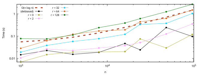
Figure 1: The runtime cost of assembling the approximation $\mathbb{\mathcal{F}}\bm{\Sigma}\mathbb{\mathcal{F}}^{H}\approx\bm{D}+\bm{U}\bm{V}^{H}$ for various different ranks $r$. For additional context, we provide the runtime cost of assembling just the diagonal matrix of $S(\omega)$ at Fourier frequencies (teal) and the diagonal matrix corresponding to the debiased Whittle estimator, which requires one FFT-based discrete convolution.

Figure 1 shows the runtime cost of assembling $\bm{D}+\bm{U}\bm{V}^{H}$ for a variety of data sizes ranging from $n=1\,000$ to $n=96\,000$ along with a theoretical $\mathcal{O}(n\log n)$ line. As one would expect for a fixed-rank approximation assembled using a $\mathcal{O}(1)$-sized number of FFTs, the empirical agreement with the theoretical complexity is good. While there is interesting variation in runtime cost when the entire assembly runs in significantly under one second, by the time the program runtime cost approaches a second the stability of the scaling is clear.

As a second investigation, we look at the relative error in the negative log-likelihood computed with the implied approximation to (1.2). This study, summarized in Figure 2, clearly demonstrates the way that this approximation depends on the specific spectral density being modeled. For $S_{1}$, we see that even a rank of $r=2$ provides an effectively exact log-likelihood with $14+$ digits of precision. The second two sub-plots in Figure 2 show two different applications of $S_{2}$. The center figure shows the relative accuracy of the negative log-likelihood when one does not correct the asymptotic expansion for the rough point at the origin when computing the autocovariance sequence $\left\{h_{k}\right\}_{k=0}^{n-1}$, instead simply pretending that the function has many derivatives everywhere. In this work the asymptotic expansions were used for $k>2\,000$, and it is clear in the figure that as soon as those expansions start being used that one goes from $14$ digits in the rank $r=128$ case to $8$ digits, and the quality of the approximation does not meaningfully improve even as the rank varies by an order of magnitude.

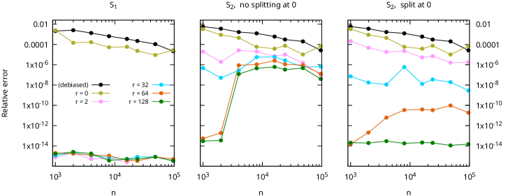
Figure 2: The relative errors in the negative log-likelihood (1.2) for various models, ranks, and data sizes. The middle column shows the error in naively applying the asymptotic expansion method of Proposition 2 to obtain $\left\{h_{k}\right\}_{k=0}^{n-1}$ despite $S(\omega)$ having zero derivatives at the origin, and the right column applies the splitted expansion method from Corollary 1.

The final panel in Figure 2 shows the relative error of the likelihood approximation (1.2) with the corrected asymptotic expansion that applies Corollary 1 at the splitting point $\omega_{1}=0$. Here we now see that there is no visible loss in accuracy once the expansions start being used for tails of the autocovariance sequence, indicating that the domain-splitting correction restores the accuracy of the expansions. As the theory would imply and this figure empirically demonstrates, the rank of the “Whittle correction” depends on properties of the spectral density. In this particular case, a rank of $r\approx 100$ is necessary to get almost every significant digit of the log-likelihood. This low rank makes sense in light of Section 3’s asymptotic expansion argument, as $S_{2}(\omega)$ is non-smooth at the origin and at the periodic endpoints.

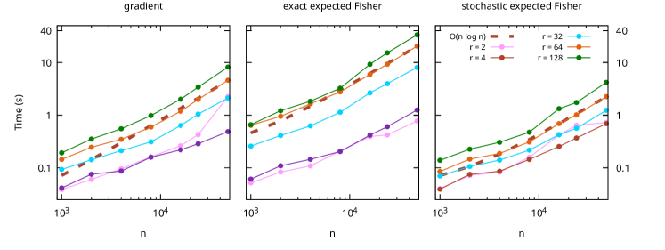
Figure 3: Runtime costs for evaluating the approximated gradient (5.2), the exact Fisher information matrix (5.3), and the symmetrized stochastic expected Fisher information matrix for various data sizes and ranks using $S_{2}(\omega)$.

Finally, we validate the runtime cost and accuracy of the gradient, the exact expected Fisher matrix, and the symmetrized stochastic expected Fisher matrix of the negative log-likelihood, although due to the exact values requiring matrix-matrix products we now only test to matrices of size $48\,000$. Figure 3 provides a summary of the runtime cost of computing the three quantities. As can be seen, the agreement with the theoretically expected $\mathcal{O}(n\log n)$ is clear. And even for $n\approx 50\,000$ data points, we see that the gradient of the likelihood—which requires a matrix-matrix product for each term—can be computed to full precision in under ten seconds. By virtue of requiring only matrix-vector products, which are exceptionally fast with this simple low-rank structure, the symmetrized stochastic expected Fisher information matrix is actually slightly faster to compute than the gradient. Each term of the exact expected Fisher information matrix requires a product of four matrices, and so the prefactor of the $\mathcal{O}(n\log n)$ complexity is significantly higher, with the rank $r=128$ value for $n=48\,000$ taking about $40$ seconds compared to the $\approx 5\text{s}$ that its stochastic counterpart required. This is of course more expensive, but it is also sufficiently manageable that one oculd certainly compute it once to high accuracy to obtain the true asymptotic precision of the MLE once the estimate $\hat{\bm{\theta}}_{\text{MLE}}$ has been computed, for example.

To study the accuracy of these approximations, Figure 4 shows two quantities. Letting $\bm{g}(\bm{\theta})$ denote the true gradient $\nabla\ell(\bm{\theta}\,|\,\bm{y})$ and $\tilde{\bm{g}}(\bm{\theta})$ denote the approximated gradient $\nabla\tilde{\ell}(\bm{\theta}\,|\,\bm{y})$, the top row shows a standard max-norm type metric of

$$\max_{j=1,...,p}\frac{\left|g_{j}(\bm{\theta})-\tilde{g}_{j}(\bm{\theta})\right|}{\left|g_{j}(\bm{\theta})\right|}$$

for models $S_{1}(\omega)$ and $S_{2}(\omega)$. Letting $\bm{I}$ denote the true expected Fisher information matrix and $\tilde{\bm{I}}$ denote the approximated one (with just the approximated $\bm{\Sigma}$ or additionally by using the stochastic trace estimator), the second row of Figure 4 shows the relative operator norm error $\left\|\bm{I}\right\|^{-1}\left\|\bm{I}-\tilde{\bm{I}}\right\|,$ which is arguably a more relevant metric for a Hessian approximation than a pointwise max-norm.

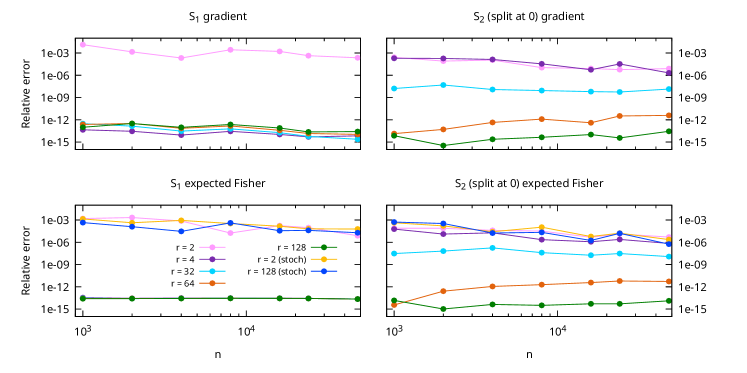
Figure 4: Relative error-type metrics for the approximated gradient and symmetrized stochastic Fisher information matrix for various ranks and sizes using $S_{2}(\omega)$.

Many of the conclusions from examining the relative error in the log-likelihood above still apply here. As before, for spectral density $S_{1}$ the matrix $\bm{\Sigma}$ is so well-behaved that even a rank $r=4$ approximation to $\mathbb{\mathcal{F}}\bm{\Sigma}\mathbb{\mathcal{F}}^{H}-\bm{D}$ and its derivatives gives $12+$ digits of accuracy in the gradient and exact expected Fisher matrix. For the likelihood of $S_{2}$, due to the roughness at the origin the rank of the Whittle correction again needs to be increased. But as one would hope, since a rank of $r=128$ gave effectively every digit in the log-likelihood, it also gives effectively every digit in the gradient and exact expected Fisher matrix. Considering that the derivatives of $S_{1}$ and $S_{2}$ with respect to $\theta_{2}$ are not strictly non-negative, this also provides a verification that the structure this method exploits works equally well for symmetric Toeplitz matrices that are not positive-definite.

For the stochastic expected Fisher matrix, every trace approximation was done using $M=72$ SAA vectors and the SAA-induced error is clearly the dominant source of disagreement with the true expected Fisher matrix, even for $r=2$. While it is tempting conclude that one could simply set $r=2$ and obtain a good estimator for the expected Fisher information matrix in under a second even for $n=50\,000$ data points, which may well be true in plenty of circumstances, the situation can be slightly more complicated than that. When using exact matrices $\bm{\Sigma}$, $\bm{\Sigma}_{j}$, and $\bm{\Sigma}_{k}$, the symmetrized stochastic estimator is an unbiased estimator. And while the SAA-induced variability in the approximated expected Fisher using the matrix approximation here may be much larger than the bias induced by setting the rank $r$ too small, the estimator now having some amount of bias may be a potential source of issues, so we advise practitioners to reduce $r$ from what they deemed necessary for an accurate log-likelihood with caution.

7 Discussion

This work introduces a pleasingly simple approximation for the covariance matrix of the DFT of a stationary time series, which incidentally may provide useful methods to a much broader range of settings where one encounters symmetric Toeplitz matrices whose diagonal sequences have well-behaved Fourier transforms. In many settings and more general Gaussian process applications, for example with irregular locations or in multiple dimensions, low rank-type methods are known to have severe limitations [22]. And for purely approximating the Toeplitz matrix $\bm{\Sigma}$, many of those issues would still be present, so it is interesting to observe that conjugating with the DFT matrix changes the algebraic structure of $\bm{\Sigma}$ to the degree where a low-rank perturbation of a diagonal matrix represents $\mathbb{\mathcal{F}}\bm{\Sigma}\mathbb{\mathcal{F}}^{H}$ to almost every achievable significant digit at double precision.

The theory in Section 3 provides a new and complementary perspective to existing analyses of the accuracy of Whittle approximations. In [24], for example, a theoretical analysis of spectral-domain approximations is provided where error is characterized by an integer $K$ and the assumption that the corresponding covariance sequence has a finite $K$-th moment $\sum_{j}j^{K}h_{j}<\infty$. This work, on the other hand, discusses non-smooth points of spectral densities and large high-order derivatives as the principle source of error. These are of course intimately connected, and the correspondence of a function’s decay rate with the smoothness of its Fourier transform is well-known. If one is designing parametric models via the spectral density, the considerations that this work motivatives for designing models that can be approximated well—namely, selecting and designing the number of non-smooth points, including at endpoints, and deciding on the magnitude of quantities like $\int_{-1/2}^{1/2}S^{(m)}(\omega)e^{2\pi i\omega k}\mathop{}\!\mathrm{d}\omega$—may be more direct in some circumstances.

Many methods already exist for exploiting structure in covariance matrices like $\bm{\Sigma}$ and achieving similar or even slightly better runtime complexity. [8] provides a hierarchically semi-separable-type (HSS) approximation to covariance matrices $\bm{\Sigma}$ that runs in linear time, and [10, 11] use hierachically off-diagonal low-rank structure (HODLR) to achieve quasilinear complexity that is comparable to that of this work. Many other hierarchical matrix formats exist [6], and in some cases can be pushed to a similar degree of accuracy as the method presented here. What makes this structure representation interesting, in our opinion, is its simplicity. This approximation is easy to implement in software (and the released code can be inspected to prove that point), and the resulting $\bm{D}+\bm{U}\bm{V}^{H}$ has a very transparent structure. Moreover, its runtime complexity is very simple and predictable since it is only controlled by one tuning parameter (the rank $r$). Despite this, it achieves high accuracy for a very broad class of spectral densities. And for users who are so inclined, making its rank adaptive would be a very simple modification to the code, following, for example, guidelines from [17]. Moreover, error control and analysis for this structure is much more direct than in a more general hierarchical matrix format, which must control the error of individual low rank approximations of off-diagonal blocks.

With that said, there are of course circumstances in which the cost of using this log-likelihood evaluation strategy is not worth the higher prefactor than, say, the debiased Whittle approximation [25]. If one has a dataset with $50\,000$ measurements that needs to be fitted once, for example, it is probably worth spending an entire two to three minutes to obtain an effectively exact MLE instead of the $15$ seconds it might take to obtain an approximate estimator from, say, the debiased Whittle method. Or at the least, it is likely worth refining that more computationally expedient estimator using the more accurate methods introduced here. But for an online application, on the other hand, or a setting in which one must fit tens or hundreds of datasets, a much cheaper method that runs in seconds instead of minutes may be worth the potential efficiency cost.

References

- Ambikasaran et al. [2014] S. Ambikasaran, M. O’Neil, and K.R. Singh. Fast symmetric factorization of hierarchical matrices with applications. arXiv preprint arXiv:1405.0223, 2014.
- Ambikasaran et al. [2015] S. Ambikasaran, D. Foreman-Mackey, L. Greengard, D.W. Hogg, and M. O’Neil. Fast direct methods for gaussian processes. IEEE transactions on pattern analysis and machine intelligence, 38(2):252–265, 2015.
- Anitescu et al. [2012] M. Anitescu, J. Chen, and L. Wang. A matrix-free approach for solving the parametric gaussian process maximum likelihood problem. SIAM Journal on Scientific Computing, 34(1):A240–A262, 2012.
- Avron and Toledo [2011] H. Avron and S. Toledo. Randomized algorithms for estimating the trace of an implicit symmetric positive semi-definite matrix. Journal of the ACM (JACM), 58(2):1–34, 2011.
- Bezanson et al. [2017] J. Bezanson, A. Edelman, S. Karpinski, and V.B. Shah. Julia: A fresh approach to numerical computing. SIAM review, 59(1):65–98, 2017.
- Börm et al. [2003] S. Börm, L. Grasedyck, and W. Hackbusch. Introduction to hierarchical matrices with applications. Engineering analysis with boundary elements, 27(5):405–422, 2003.
- Brockwell and Davis [1991] P.J. Brockwell and R.A. Davis. Time series: theory and methods. Springer science & business media, 1991.
- Chen and Stein [2023] J. Chen and M.L. Stein. Linear-cost covariance functions for gaussian random fields. Journal of the American Statistical Association, 118(541):147–164, 2023.
- Deaño et al. [2017] A. Deaño, D. Huybrechs, and A. Iserles. Computing highly oscillatory integrals. SIAM, 2017.
- Foreman-Mackey et al. [2017] D. Foreman-Mackey, E. Agol, S. Ambikasaran, and R. Angus. Fast and scalable gaussian process modeling with applications to astronomical time series. The Astronomical Journal, 154(6):220, 2017.
- Geoga et al. [2020] C.J. Geoga, M. Anitescu, and M.L. Stein. Scalable gaussian process computations using hierarchical matrices. Journal of Computational and Graphical Statistics, 29(2):227–237, 2020.
- Gonnet [2012] P. Gonnet. A review of error estimation in adaptive quadrature. ACM Computing Surveys (CSUR), 44(4):1–36, 2012.
- Gray [2006] R.M. Gray. Toeplitz and circulant matrices: A review. Foundations and Trends® in Communications and Information Theory, 2(3):155–239, 2006.
- Greengard and Rokhlin [1987] L. Greengard and V. Rokhlin. A fast algorithm for particle simulations. Journal of computational physics, 73(2):325–348, 1987.
- Greengard and Strain [1991] L. Greengard and J. Strain. The fast gauss transform. SIAM Journal on Scientific and Statistical Computing, 12(1):79–94, 1991.
- Greengard et al. [2007] L. Greengard, J.Y. Lee, and S. Inati. The fast sinc transform and image reconstruction from nonuniform samples in k-space. Communications in Applied Mathematics and Computational Science, 1(1):121–131, 2007.
- Halko et al. [2011] N. Halko, P.G. Martinsson, and J.A. Tropp. Finding structure with randomness: Probabilistic algorithms for constructing approximate matrix decompositions. SIAM review, 53(2):217–288, 2011.
- Heyde [1997] C.C. Heyde. Quasi-likelihood and its application: a general approach to optimal parameter estimation. Springer, 1997.
- Johnson [2013] S.G. Johnson. QuadGK.jl: Gauss–Kronrod integration in Julia. https://github.com/JuliaMath/QuadGK.jl, 2013.
- Litvinenko et al. [2019] A. Litvinenko, Y. Sun, M.G. Genton, and D.E. Keyes. Likelihood approximation with hierarchical matrices for large spatial datasets. Computational Statistics & Data Analysis, 137:115–132, 2019.
- Minden et al. [2017] V. Minden, A. Damle, K.L. Ho, and L. Ying. Fast spatial gaussian process maximum likelihood estimation via skeletonization factorizations. Multiscale Modeling & Simulation, 15(4):1584–1611, 2017.
- Stein [2014] M.L. Stein. Limitations on low rank approximations for covariance matrices of spatial data. Spatial Statistics, 8:1–19, 2014.
- Stein et al. [2013] M.L. Stein, J. Chen, and M. Anitescu. Stochastic approximation of score functions for gaussian processes. The Annals of Applied Statistics, pages 1162–1191, 2013.
- Subba Rao and Yang [2021] S. Subba Rao and J. Yang. Reconciling the gaussian and whittle likelihood with an application to estimation in the frequency domain. The Annals of Statistics, 49(5):2774–2802, 2021.
- Sykulski et al. [2019] A.M. Sykulski, S.C. Olhede, A.P. Guillaumin, J.M. Lilly, and J.J. Early. The debiased whittle likelihood. Biometrika, 106(2):251–266, 2019.
- Thomson [1982] D.J. Thomson. Spectrum estimation and harmonic analysis. Proceedings of the IEEE, 70(9):1055–1096, 1982.
- Trefethen [2019] L.N. Trefethen. Approximation theory and approximation practice, extended edition. SIAM, 2019.
- Tropp and Webber [2023] J.A. Tropp and R.J. Webber. Randomized algorithms for low-rank matrix approximation: Design, analysis, and applications. arXiv preprint arXiv:2306.12418, 2023.
- Wood and Chan [1994] A.T.A. Wood and G. Chan. Simulation of stationary gaussian processes in [0, 1] d. Journal of computational and graphical statistics, 3(4):409–432, 1994.