Generalized Step-Chirp Sequences With Flexible Bandwidth
Abstract
Sequences with low aperiodic autocorrelation sidelobes have been extensively researched in literatures. With sufficiently low integrated sidelobe level (ISL), their power spectrums are asymptotically flat over the whole frequency domain. However, for the beam sweeping in the massive multi-input multi-output (MIMO) broadcast channels, the flat spectrum should be constrained in a passband with tunable bandwidth to achieve the flexible tradeoffs between the beamforming gain and the beam sweeping time. Motivated by this application, we construct a family of sequences termed the generalized step-chirp (GSC) sequence with a closed-form expression, where some parameters can be tuned to adjust the bandwidth flexibly. In addition to the application in beam sweeping, some GSC sequences are closely connected with Mow’s unified construction of sequences with perfect periodic autocorrelations, and may have a coarser phase resolution than the Mow sequence while their ISLs are comparable.
I Introduction
Sequences with low aperiodic autocorrelation sidelobes are desirable in communications and radar engineering, e.g., some of the chirp-like sequences developed in [1, 2, 3, 4, 5]. With a low integrated sidelobe level (ISL), these sequences have quite flat spectrums [6], which can be utilized to achieve omnidirectional precoding in broadcast channels [7].
In 5G NR broadcast channels, the discrete Fourier transform (DFT) codebook is adopted for broadcasting common messages [8, Section 6.1.6.3] in the initial stage of communication. With the energy concentrated in the pointing direction, the maximum beamforming gain can be achieve by the DFT codebook. But for future wireless communication systems with massive number of antennas, the resultant beam would be too narrow, thus requiring many times of beam sweeping to cover the whole angular domain. In contrast, the chirp-like sequence-based omnidirectional beamforming spreads the energy in the whole angular domain, and thus avoids beam sweeping and improves the time efficiency. The omnidirectional beamforming, however, has no beamforming gain, and therefore may have insufficient range coverage for the millimeter-wave or terahertz-wave communication systems where a high beamforming gain is required for compensating the severe path loss.
To circumvent such a dilemma, it is desirable to achieve flexible tradeoffs between the beamforming gain and the beam sweeping time, as pursued by the 3GPP [9]. From the aspect of spectrum, we aim at designing sequences whose power variation in the passband and power leakage in the stopband should be as small as possible, and the bandwidth of the passband should be flexibly tunable. Besides, their entries should have equal amplitudes for maximizing the energy efficiency of power amplifiers (PAs), and their phase resolutions should be coarse for the implementation using a low-cost phase shifter network (PSN).
Literatures on this topic include some numerical optimizations [10, 11, 12] and some schemes with closed-form solutions [9, 13, 14, 15, 16]. Compared with the numerical optimizations, the schemes with closed-form solutions are easier for hardware implementation, but the bandwidth is less flexible except for the scheme in [15]. The sequence inferred from [15], referred to as the generalized chirp (GC) sequence in this paper, has flexible bandwidth the same as the numerical counterparts, and its spectrum in the passband is asymptotically flat [15]. Nevertheless, for the GC sequence, the phase resolution of the PSN is too fine to be cost-effective when the number of antennas is large, as shown in our simulations.
In recent years, polyphase sequences with low correlations and spectrally-null constraints were constructed in [17, 18, 19, 20], whose -point spectrums (with being the sequence length) are ideally flat in the passbands and are ideally null in the stopbands. Nevertheless, the -point spectrum is insufficient for beamforming because the user equipments (UEs) are distributed in a continuous angular range, rather than the discrete directions. Besides, the passbands are interleaved with the stopbands [20] and the bandwidths are less flexible. Hence, they are still not suitable for beam sweeping.
To achieve flexible tradeoffs between the beamforming gain and the beam sweeping time, in this paper we construct a family of polyphase sequences with flexible bandwidth, termed as the generalized step-chirp (GSC) sequence. The GSC sequence enjoys a coarser phase resolution than the GC sequence. Besides, when the passband stretches over the whole frequency domain, the GSC sequence degenerates into a low-ISL sequence closely connected with the Mow sequence [5] with perfect periodic autocorrelation, and may require a coarser phase resolution than the Mow sequence.
Notations: stands for taking the floor value. represents the set of positive integers, . . is the Frobenius norm. For , stands for that is an integer multiple of ; means that is an integer multiple of and ; is equivalent to .
II Preliminaries
In this section, we review two kinds of passive beamformings for the common message broadcasting: the conventional beam sweeping based on the DFT codebook [8, Section 6.1.6.3] in Section II-A and the omnidirectional beamforming based on the chirp-like sequence [5] in Section II-B.
II-A DFT Codebook-based Beam Sweeping
Consider a uniform linear array (ULA) of isotropic antennas with half wavelength spacing. Given a beamforming vector with , the radiated power at azimuth angle and elevation angle is
| (1) |
where . Note that , hence is essentially the power spectrum of the sequence .
A DFT codeword is with , where is the beam direction in the -domain. Let , then the radiated power is
| (2) |
By (2), the maximum beamforming gain (the ratio of the maximum received power to the average received power) can be achieved if , and for a sufficiently large ,
| (3) |
i.e., is closed to the half-power points of the beam. Hence the DFT codeword is designed to cover . Then a DFT codebook with is adopted to sweep the beam over the whole space for broadcasting common message, as illustrated by Fig. 1 (a). The beam sweeping would consume too many time slots if is large.
II-B Chirp-like Sequence-based Omnidirectional Beamforming
In contrast to the beam sweeping that requires many time slots, the omnidirectional beamforming aims at broadcasting messages using only one time slot, which can be achieved by designing a sequence with a flat power spectrum.
Definition 1
For a length- complex sequence with , its aperiodic autocorrelation is defined as
| (4) |
where if or , and the overbar represents the complex conjugation.
The power spectrum of is
| (5) |
and the variance of the power spectrum is
| (6) | ||||
where is the integrated sidelobe level (ISL) of . Hence for omnidirectional beamforming, the sequence ’s ISL should be small, e.g., some of the chirp-like sequences [1, 2, 3, 4, 5]. As a unified construction of sequences with perfect periodic autocorrelation, the Mow sequence family [5] where some sequences have low ISL, is given below for ease of reference.
Definition 2
[5] The Mow sequence is a kind of sequences of length with being the square-free part of , whose entries are with
| (7) |
where
| (8) |
is any function with , and is any function such that is a permutation of , and are any rational numbers.
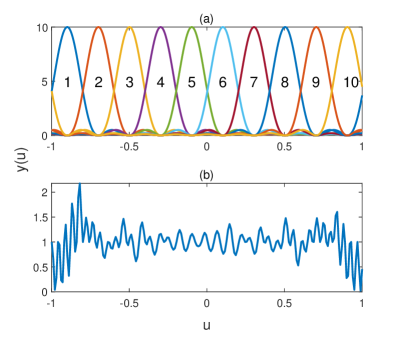
The beam sweeping based on the DFT codebook and the omnidirectional beamforming based on the Mow sequence are compared in Fig. 1. For the DFT codebook, ; for the Mow sequence, , , , , , , . The DFT codebook in Fig. 1 (a) achieves the maximum beamforming gain but requires times of beam sweeping, while the Mow sequence in Fig. 1 (b) can broadcast messages in one time slot but has no beamforming gain.
III Generalized Step-chirp Sequence
To achieve flexible tradeoffs between the beamforming gain and the beam sweeping time, in Section III-A, we construct a family of polyphase sequences with tunable bandwidth, termed as the generalized step-chirp (GSC) sequence; in Section III-B, we discuss the relationships between the GSC sequence, the DFT codebook, the generalized chirp (GC) sequence inferred from [15] and the Mow sequence [5].
III-A Construction of Generalized Step-chirp Sequence
Consider a step-chirp signal as follows:
| (9) |
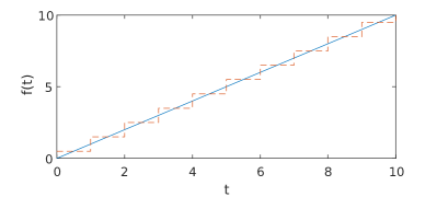
where is a step approximation of linear frequency modulation (LFM):
| (10) |
for . An LFM and its step approximation with , and are illustrated by Fig. 2. The bandwidth of the step-chirp signal is approximately. Besides, we require the Nyquist sampling number .
Now sample in (9) at rate with , where is assumed to be an integer via setting properly. We then obtain samples
| (11) |
with
| (12) |
Because , we have .
Besides, the Fourier transform of can be derived to be a weighted summation of sinc functions:
| (16) |
At , the value of the left-most sinc function () is ; at , the value of the right-most sinc function () is . Hence the interval can be regarded as the stopband since most of the sinc functions have attenuated to a low level. Because the bandwidth of the step-chirp signal is approximately, the interval can be regarded as the passband of . Note that the analog bandwidth is scaled to be the digital bandwidth by over-sampling, hence the passband of the sample sequence is where
| (17) |
The above arguments established the following theorem.
Theorem 1
The GSC sequence is a family of polyphase sequences with entries , where
| (18) | ||||
with parameter set . The passband of the power spectrum of the GSC sequence is
| (19) |
where . For beam sweeping, the beam is pointed at to cover , where
| (20) |
The bandwidth of the GSC sequence can be flexibly adjusted by tuning the parameter , thus achieving the flexible tradeoffs between the beamforming gain and the beam sweeping time, as shown in Simulations.
III-B Relationships Between the GSC sequence and Other Sequences
The relationships between the GSC sequence, the DFT codebook, the GC sequence and the Mow sequence family are illustrated by Fig. 3, as explained below.
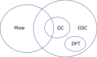
III-B1 GSC Sequence and DFT Codebook
In Theorem 1, let and . Then we have and for . This degenerated GSC sequence has entries
| (21) |
and the passband is
| (22) |
According to Section II-A, this is exactly a DFT codeword pointing at . Hence the GSC sequence encompasses the DFT codebook and thus may be backward-compatible with the current industrial standard.
III-B2 GSC Sequence and GC Sequence
When , we have from (18) that , which is the GC sequence inferred from over-sampling a chirp signal [15]. Therefore, the GSC sequence is also a generalization of the GC sequence. The phase resolution of a sequence with phases in is . Note that the parameter can be tuned for coarser phase resolution, e.g., suppose and is a rational number of form with coprime, then the phase resolutions are
| (23) |
from which we have , e.g., if , then .
III-B3 GSC Sequence and Mow Sequence
Set (i.e., the Nyquist sampling), and we obtain another kind of degenerated GSC sequence with entries , where
| (24) | ||||
with parameter set , which is related to the Mow sequence as shown below.
Proposition 1
Proof:
First note that with the first constraint, the sequence length in (24) is , which is the same as the Mow sequence.
Indeed, one may relax the constraints in Proposition 1 to improve the phase resolution of the degenerated GSC sequence in (24). The phase resolution of the Mow sequence in (7) with being an integer is
| (28) |
and the phase resolution of the GSC sequence with is . If is larger than the square part of , then the phase resolution of the GSC sequence would be coarser than the Mow sequence as shown in Simulations.
IV Simulations
This section presents simulation examples to verify the capability of the GSC sequence in making flexible tradeoffs between the beamforming gain and the beam sweeping time, and its advantages over the GC sequence and the Mow sequence in terms of the phase resolution and the spectrum.
IV-A Tradeoffs Between the Beamforming Gain and the Beam Sweeping Time
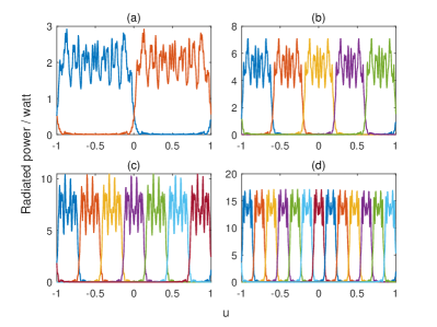
To show the flexibility of the GSC sequence for beam sweeping, we simulate and show in Fig. 4 the beampatterns of the GSC sequences of length with . The parameter is chosen so that the beam direction in (20) runs through for the contiguous coverage of . Fig. 4 (a) illustrates times of beam sweeping with 2x beamforming gain while Fig. 4 (d) represents times of beam sweeping with 13x beamforming gain. In summary, by adjusting and to control the bandwidth and the beam direction, flexible tradeoffs between the beamforming gain and the beam sweeping time can be achieved for efficient beam sweeping. We want to emphasize that the y-axis is in the linear scale. Thus, the power fluctuation in the passband is less than dB.
IV-B Phase Resolution and Spectrum
For a GSC sequence , the normalized root mean square error (NRMSE) of passband is defined as
| (29) |
where is the DFT length and is the set of passband indices. Here we set . And the stopband leakage ratio is defined as
| (30) |
where is the set of the stopband indices.
Compared with the GC sequence and the Mow sequence, the GSC sequence with a proper parameter may have a coarser phase resolution and a comparable spectrum or even flatter.
IV-B1 GSC Sequence versus GC sequence
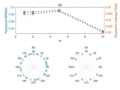
Fig. 5 shows the impact of the parameter on the spectrum and the phase resolution of a GSC sequence, where , , . Compared with the GC sequence, i.e., , the GSC sequence with has smaller passband NRMSE and stopband leakage ratio as shown in Fig. 5 (a), and the phase resolution of the proposed GSC sequence is times coarser as shown in Fig. 5 (b) and Fig. 5 (c).
IV-B2 GSC sequence versus Mow sequence
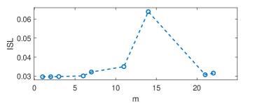
Fig. 6 shows the ISL of a GSC sequence of length for different parameters , with and . Note that the square part of is , thus the point with in Fig. 6 corresponds to a Mow sequence, which can be verified by simulation to have exactly the minimum ISL among all the Mow sequences of length with a phase resolution [5, Theorem 5]. Remarkably, the ISL for is and the ISL for is , which means a reduction of phase resolution by a factor of but with a negligible increase of ISL, i.e., a comparably flat spectrum.
V Conclusions
In this paper, we construct the generalized step-chirp (GSC) sequence, which can achieve flexible tradeoffs between the beamforming gain and the beam sweeping time for the common message broadcasting in massive MIMO systems. The GSC sequence has a coarser phase resolution than the generalized chirp (GC) sequence, which facilitates its implementation with a low-cost phase shifter network (PSN). Besides, the GSC sequence may have coarser phase resolution than the Mow sequence with a negligible increase of the integrated sidelobe level (ISL).
References
- [1] R. Frank, “Polyphase codes with good nonperiodic correlation properties,” IEEE Transactions on Information Theory, vol. 9, no. 1, pp. 43–45, 1963.
- [2] D. Chu, “Polyphase codes with good periodic correlation properties (corresp.),” IEEE Transactions on information theory, vol. 18, no. 4, pp. 531–532, 1972.
- [3] A. Milewski, “Periodic sequences with optimal properties for channel estimation and fast start-up equalization,” IBM Journal of Research and Development, vol. 27, no. 5, pp. 426–431, 1983.
- [4] B. M. Popovic, “Generalized chirp-like polyphase sequences with optimum correlation properties,” IEEE Transactions on Information Theory, vol. 38, no. 4, pp. 1406–1409, 1992.
- [5] W. H. Mow, “A new unified construction of perfect root-of-unity sequences,” in Proceedings of ISSSTA’95 International Symposium on Spread Spectrum Techniques and Applications, vol. 3. IEEE, 1996, pp. 955–959.
- [6] K.-U. Schmidt, “On a problem due to Littlewood concerning polynomials with unimodular coefficients,” Journal of Fourier Analysis and Applications, vol. 19, no. 3, pp. 457–466, 2013.
- [7] X. Meng, X. Xia, and X. Gao, “Omnidirectional space-time block coding for common information broadcasting in massive mimo systems,” IEEE Transactions on Wireless Communications, vol. 17, no. 3, pp. 1407–1417, March 2018.
- [8] 3GPP, “Study on new radio access technology physical layer aspects,” 3GPP, Technical Specification (TS) TS38.802 V14.2.0, Sept. 2017.
- [9] Intel, “Codebook with beam broadening,” 3GPP, Tech. Rep. R1-1611929, Nov. 2016.
- [10] W. Rowe, P. Stoica, and J. Li, “Spectrally constrained waveform design [sp tips&tricks],” IEEE Signal Processing Magazine, vol. 31, no. 3, pp. 157–162, 2014.
- [11] V. Sergeev, A. Davydov, G. Morozov, O. Orhan, and W. Lee, “Enhanced precoding design with adaptive beam width for 5G new radio systems,” in 2017 IEEE 86th Vehicular Technology Conference (VTC-Fall). IEEE, 2017, pp. 1–5.
- [12] W. Ma, L. Zhu, and R. Zhang, “Passive beamforming for 3-D coverage in IRS-assisted communications,” IEEE Wireless Communications Letters, vol. 11, no. 8, pp. 1763–1767, 2022.
- [13] Z. Xiao, T. He, P. Xia, and X.-G. Xia, “Hierarchical codebook design for beamforming training in millimeter-wave communication,” IEEE Transactions on Wireless Communications, vol. 15, no. 5, pp. 3380–3392, 2016.
- [14] Z. Xiao, H. Dong, L. Bai, P. Xia, and X.-G. Xia, “Enhanced channel estimation and codebook design for millimeter-wave communication,” IEEE Transactions on Vehicular Technology, vol. 67, no. 10, pp. 9393–9405, 2018.
- [15] C. Fonteneau, M. Crussière, and B. Jahan, “A systematic beam broadening method for large phased arrays,” in 2021 Joint European Conference on Networks and Communications & 6G Summit (EuCNC/6G Summit). IEEE, 2021, pp. 7–12.
- [16] C. Du, F. Li, and Y. Jiang, “Hierarchical beamforming for broadcast channels,” IEEE Communications Letters, 2023.
- [17] S. Hu, Z. Liu, Y. L. Guan, W. Xiong, G. Bi, and S. Li, “Sequence design for cognitive cdma communications under arbitrary spectrum hole constraint,” IEEE Journal on Selected Areas in Communications, vol. 32, no. 11, pp. 1974–1986, 2014.
- [18] Z. Liu, Y. L. Guan, U. Parampalli, and S. Hu, “Spectrally-constrained sequences: Bounds and constructions,” IEEE Transactions on Information Theory, vol. 64, no. 4, pp. 2571–2582, 2018.
- [19] L. Tian, C. Xu, and Y. Li, “A family of single-channel spectrally-null-constrained sequences with low correlation,” IEEE Signal Processing Letters, vol. 27, pp. 1645–1649, 2020.
- [20] Z. Ye, Z. Zhou, Z. Liu, X. Tang, and P. Fan, “New spectrally constrained sequence sets with optimal periodic cross-correlation,” IEEE Transactions on Information Theory, vol. 69, no. 1, pp. 610–625, 2022.