NeuroKoopman Dynamic Causal Discovery
Abstract
In many real-world applications where the system dynamics has an underlying interdependency among its variables (such as power grid, economics, neuroscience, omics networks, environmental ecosystems, and others), one is often interested in knowing whether the past values of one time series influences the future of another, known as Granger causality, and the associated underlying dynamics. This paper introduces a Koopman-inspired framework that leverages neural networks for data-driven learning of the Koopman bases, termed NeuroKoopman Dynamic Causal Discovery (NKDCD), for reliably inferring the Granger causality along with the underlying nonlinear dynamics. NKDCD employs an autoencoder architecture that lifts the nonlinear dynamics to a higher dimension using data-learned bases, where the lifted time series can be reliably modeled linearly. The lifting function, the linear Granger causality lag matrices, and the projection function (from lifted space to base space) are all represented as multilayer perceptrons and are all learned simultaneously in one go. NKDCD also utilizes sparsity-inducing penalties on the weights of the lag matrices, encouraging the model to select only the needed causal dependencies within the data. Through extensive testing on practically applicable datasets, it is shown that the NKDCD outperforms the existing nonlinear Granger causality discovery approaches.
Index Terms:
Granger causality, Time series, Koopman operator, Nonlinear dynamics1 Introduction
1.1 Motivation and Related Works
Causality analysis is vital in multivariate time series study for identifying potential cause and effect-informed networked dynamic relationships present in the observational data [1]. Granger causality (GC) corresponds to the situation in which the past of one time series helps predict the future of another [2, 3]. The notion of GC has been utilized in many fields of networked dynamics, including finance [4], neuroscience [5], meteorology [6], economics [7]. In neuroscience [8, 9] and biology [10, 11], for example, such analyses help determine whether a past activity in one brain region influences a later activity in another region, and to infer the underlying gene regulatory networks, respectively.
Many traditional methods for estimating GC assume that the time series follows linear dynamics and thus use a vector autoregressive (VAR) model [11, 3], where for a vector of variables at time , ), the following linear regression holds:
| (1) |
Here are lag matrices, is the maximum lag (“memory of the system”), and is additive noise, typically assumed to be a zero mean white noise. GC dependency then corresponds to the non-zero entries in . Authors in [12] later gave an equivalent definition of GC based on coefficients in a moving average (MA) representation (see [13]). GC for an pair can be tested statistically using an -test [14] comparing two models: an estimated model, which includes past values of both and versus another estimated model, that includes the past values of only . is declared Granger causal for if the -test hypothesis of ’s dependence on is accepted.
Sparsity-inducing regularizers, such as lasso [15] or group lasso [16], are used to identify the minimally required number of causal dependencies [11]. These regularizers result in only a limited number of GC connections for each time series. Additionally, it is necessary to define the maximum time delay to be considered in GC analysis. To address the issue of choosing the relevant number of lags without causing overfitting, methodologies such as the hierarchical [17] and truncating lassos [18] have been proposed.
When data dynamics are nonlinear, imposing linear models can lead to inconsistent estimation of the true Granger causal interactions [19, 20]. Model-free methods like transfer entropy [21] or directed information [22] avoid linearity assumption, but only infer connectivity information and not the underlying dynamics [23]. Deep Learning (DL) and ML methods have shown promise in learning the complex dynamics of a system. Neural networks (NNs) and their variants, such as autoregressive multilayer perceptrons [24, 25] (MLPs) and long-short term memory networks (LSTMs) [26], are capable of modeling nonlinear interactions [27]. However, these methods may lack interpretability if not carefully modeled. Accordingly, [28] introduced component-wise MLPs and LSTMs, termed cMLP and cLSTM, that support the interpretability of GC from the learned models. Search for parameters of these models is also coupled with sparsity-inducing penalties.
In this research, we propose our approach of inferring causal structure and underlying dynamics using a Koopman-inspired lifting of the given time series data into a higher-dimensional space where the evolution appears linear reliably; use data-driven auto-learning of the lifting and projection functions in the form of neural networks; and next infer a sparse linear regressive model in the lifted domain. The traditional approach to Koopman linear embedding employs a large number of nonlinear basis functions for approximating nonlinear systems into higher dimensional linear representations [29] and for projecting the lifted linear dynamics back to the base space [30]. However, to select the basis functions for lifting/projection, the traditional methods rely on ad hoc predefined dictionaries of bases, such as polynomial or radial functions, which may not be optimal. Some ways to obtain approximations of the Koopman operators involve utilizing the methods of dynamic mode decomposition (DMD) [31] and the extended-DMD (EDMD) [30, 32], where again, one assumes the knowledge of a predefined dictionary of basis functions. Inferring causal interactions, utilizing the Koopman embedding, is a relatively young field. Authors in [33] infer causal interaction in a dynamical system by using transfer Perron-Frobenius (P-F) and Koopman operators, whereas [34] utilized the setting of DMD towards GC inference.
In contrast to the traditional predefined basis dictionary, the data-driven approach provides a potential to learn basis functions accurately, without needing any user-designated bases [35], thereby enabling a scalable auto-encoding of the basis functions. NNs have been used to learn Koopman embeddings [36, 37]. Recently, we have also demonstrated their application to model-predictive control (MPC) of smart grids by employing auto-learned Koopman bases to accelerate MPC computation [38]. In this research, we learn the GC relation and dynamics via a linear regression applied to the nonlinearly transformed time series, employing a data-driven NN-based autoencoder for the first time:
| (2) |
where the intrinsic nonlinear lifting map , the causal interactions among the lifted variables captured by lag matrices , as well as their projection map , are all learned simultaneously in one go from the observed time series data. (The dimension of the auto-encoded lifted space is a hyperparameter and is chosen by exploration.)
1.2 Our Approach and Key Contributions
We summarize here the key contributions of our framework “NeuroKoopman Dynamic Causal Discovery (NKDCD)” with the following key contributions:
-
•
We introduce the NKDCD architecture for causal discovery and learning underlying dynamics, comprising of:
-
–
A data-driven basis-dictionary free approach to learning the NN-based bases for linear Koopman embedding required of capturing sparse nonlinear dependency in from a higher-dimensional sparse linear model (5);
-
–
A NN-based data-driven learning of sparse linear model in the lifted domain to infer GC and underlying dynamics;
-
–
A data-driven learning of projection function to map down both the lifted domain time series and the estimated high-dimensional sparse linear models to the base space.
-
–
-
•
The linear embedding approach is basis dictionary-free, in which the bases are auto-learned from the data, unlike the traditional approaches that manually pick basis functions that generally do not lead to optimal solutions.
-
•
Each element of the time series is lifted identically to its higher-dimensional representation, , thereby preserving variable-wise separation at the lifted level, to ensure variable-wise disentanglement of the signals and their interdependencies in the lifted domain.
-
•
For preserving the structure of sparsity and interdependencies of the original variables, group-level sparsity-inducing penalties are imposed in the lifted high-dimensional setting, where all lifted variables corresponding to a single variable of the original domain are placed in the same group.
-
•
The autoencoder-based architecture is trained end-to-end in one go, learning directly from data the unknown basis function, the lag matrices associated with the lifted domain model, and the projection function together while minimizing the least-square prediction error and maximizing the sparsity of interdependencies. Such an end-to-end learning also eliminates the risks of numerical issues associated with iterative learning of the individual components (lifting, lag dynamics causality, and projection) [38].
-
•
For accuracy and reliability, the loss function involves multiple terms to individually account for the accuracy of each NN block’s input-output relationship, making the overall autoencoder architecture robust. These correspond to the accuracy of the temporal dependencies, the GC constraints, and the lifting and projection functions.
-
•
Since appropriate lag selection is crucial for GC and underlying dynamics discovery, we impose additional structured group penalties that infer both the GC and the lags for each of the inferred interactions. Our formulation automatically selects a subset of the time series for each output time series that Granger causes it, regardless of the lag of the interaction.
- •
2 Mathematical Framework
As outlined in [2], the notion of Granger causal interaction is formulated as follows: A time series Granger causes time series if the variance of the prediction error when the history of is included is lower than the variance of the prediction error when the history of is excluded, i.e.,
| (3) |
where represents the history containing all relevant information prior to time , indicates the exclusion of values from , and denotes the variance. Essentially, is causal for if past values of improve the prediction of .
2.1 Traditional VAR models for GC
Considering the model of (1), a time series element Granger-causes another time series element if there exists a value at any lag for which . GC analysis thus amounts to estimating the lag matrices from the time series observations, and determining the non-zero entries. The loss function includes the square of the prediction error together with lasso penalty [43, 16] on the lag matrices to attain their sparsity:
2.2 Nonlinear autoregressive (NAR) model
The VAR model assumes linear dependence, which might not be the case for a practically applicable setting, in which case, the model may not yield the GC dependencies correctly. In practice, can evolve according to more general nonlinear dynamics. A general element-wise nonlinear autoregressive (NAR) model is of the following form [44]:
| (5) |
where is an abbreviation to denote the past values, , and is a function that specifies how the past lags are mapped to . Granger non-causality of for corresponds to the situation when does not depend on .
2.3 Proposed framework of NeuroKoopman Dynamic Causal Discovery (NKDCD)
Suppose we have an NAR time series data . We first lift each element of vector data at each time point to higher-dimensional intrinsic coordinates:
| (6) | ||||
The lifted data is then modeled following VAR as in (2):
| (7) | ||||
where ’s are the lag matrices in the lifted domain, and is the model estimate of . Both and are projected element-wise using to the base space to yield:
| (8) | |||
| (9) |
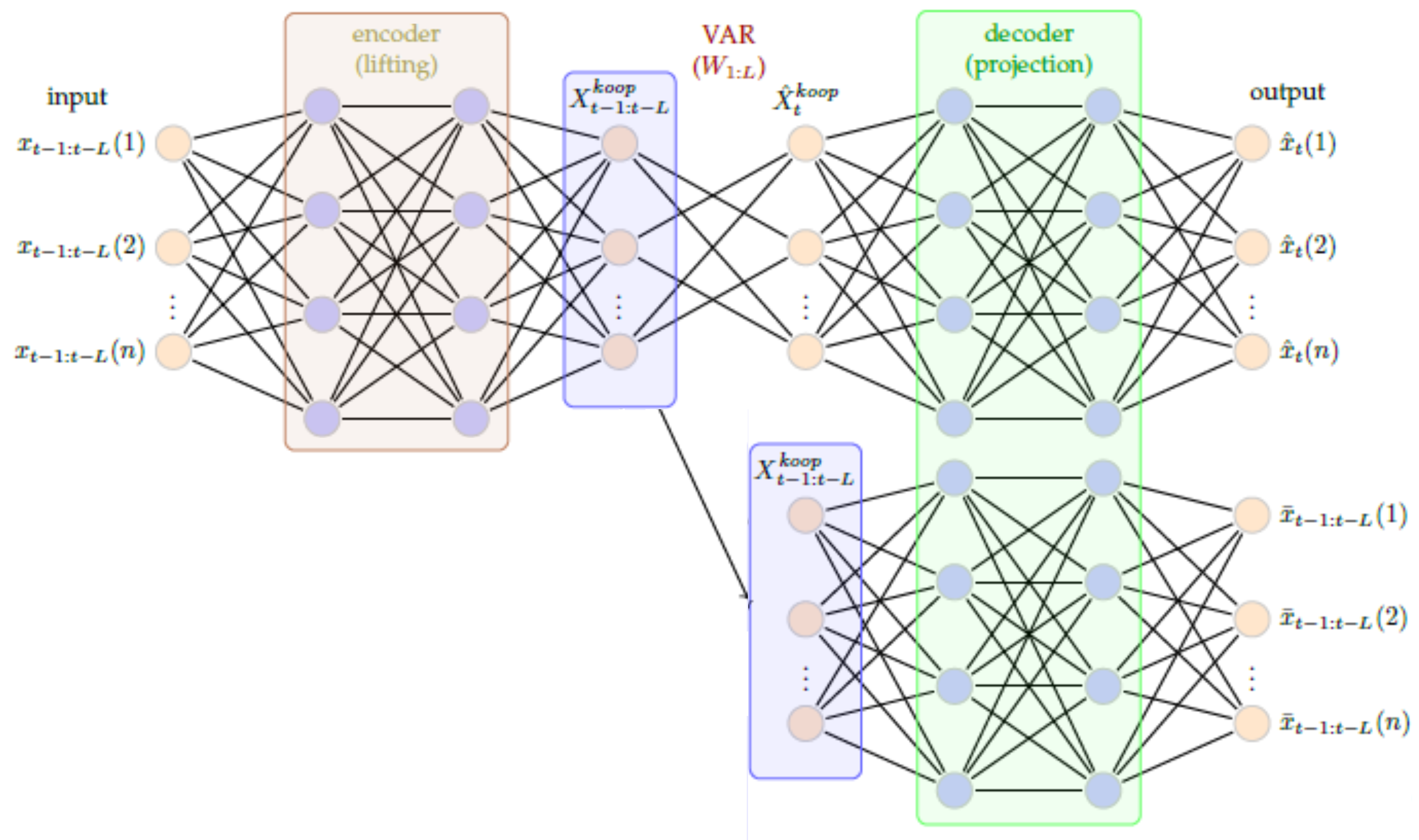
Figure 1 depicts the NKDCD architecture and labels the base, lifted, and projected variables, the encoder that performs the lifting from the base space to a higher dimensional space, the decoder that performs the opposite, and the lag matrices for linear regression in the lifted domain.
Definition 1 (NKDCD Model-based GC).
Referring to the NKDCD model (7), the time series is Granger non-causal for time series if for all , so the time series does not contribute to the prediction of the time series.
The lifting function, , the projection function, , and the lag matrices, , are learned from the observed time series data in one go. To ensure learning robustness, we define a multi-term loss function, addressing the correctness of each component of the proposed NKDCD architecture.
-
1.
Correctness of mapping to lifted space and its projection to base space: In the NKDCD framework, the dynamics evolve over the intrinsic coordinates in the lifted domain, whereas the inverse recovers the base space value. For the accuracy of the lifting and projection pair, we introduce the following loss term:
-
2.
Correctness of linear VAR model in lifted space: To discover the lag matrices that govern the GC and underlying dynamics, we learn the lag matrices over the intrinsic coordinates, so that holds. The accuracy of learning the lag matrices is achieved by introducing this loss term:
-
3.
Correctness of NAR model in base space: The projection operation allows us to map the linear VAR model of the lifted space to the NAR model of the base space. To achieve reconstruction accuracy of the NAR model, we introduce this additional loss term:
-
4.
Correctness of NAR model with autoencoder: The lifting and projection can be applied on the input side before comparing to the NAR output to enhance the end-to-end accuracy further, and for which we introduce this another loss term:
-
5.
Sparsity of GC: To have as few GC dependencies as needed, we add a fifth term to the loss function of the form , where is a tunable scalar hyperparameter, that penalizes having a large number of non-zero entries in . Since minimizing the count of non-zero entries is equivalent to minimizing the -norm, which is discrete and hence discontinuous, one instead considers a relaxation to the -norm. Since each is a matrix representing the lag- weights between the lifted components of the th time series element and the lifted components of the th time series element, all such elements of for each are grouped together, thereby the sparsity penalty becomes an -norm over groups, termed group lasso.
In addition, since all elements must be zero to ensure that is not GC dependent on , a grouping across the lags can be further employed. Grouping all the lags into a single group treats them equally, resulting in a “uniform-lag group lasso (ulg-lasso)”:
(10) The ulg-lasso of (10), however, runs the risk of treating the distant lag terms that may be absent in the ground truth the same as the near ones that are actually present in the ground truth. So a “hierarchical-lag group lasso (hlg-lasso)” that discounts more distant lags more severely is instead used sometimes:
(11) Finally, the most general case is when all the lags, near or distant, are treated independently, resulting in “independent-lag group lasso (ilg-lasso)”:
(12) Note as discussed above, the grouping in (12) corresponds to putting all elements of into its own group for each . Such grouping is also applicable to ulg- and hlg- lassos.
In summary, the overall loss function is defined as:
| (13) |
where takes the one of the forms in (10)-(12). For notational convenience, we denote the first four terms in as (which involves four -norm terms, each of which is differentiable and so allows gradient descent for loss minimization) and denote the last term in as , which being group lasso, involves inter-group -norm and intra-group -norm, that is not differentiable, requiring proximal-gradient descent for -loss minimization (in contrast, the -loss minimization uses the usual gradient descent).
In Section 3, we employ all three instances of group lasso for comparison and demonstrate how ilg-lasso outperforms hlg-lasso, which in turn surpassed ulg-lasso in performance.
2.4 Hyperparameters of NKDCD and loss function
In our autoencoder model of Figure 1, each time series is lifted to dimensions, which is one of the hyperparameters. The maximum amount of lag is , which is another hyperparameter. We have chosen the lifting and projection functions to have hidden layers, where when the data has nonlinear dynamics, each hidden layer uses the leaky rectified linear unit (leakyReLU) as the activation function: and no activation function when the data has linear dynamics. The lifting hidden layer weight sizes are parameterized by and are respectively, , , and , while the projection hidden layer weight sizes are respectively, , , and . The hyperparameter of the loss function is the sparsity weight factor . During the training of NKDCD, the learning rate (also called step-size) is yet another hyperparameter, and so is the threshold used to view a weight parameter below the threshold as zero.
2.5 NKDCD optimization: (Proximal) gradient descent
Recall the decomposition of the loss function, in which the portion of the loss function is only a function of the lag matrices , and it does not depend on the lifting and projection functions . As a result, the gradient of loss with respect to , denoted , satisfies: , and similarly, . In contrast, the gradient of vs. with respect to the lag matrices are different from each other: , because (whereas in contrast, ).
Accordingly, in the th iteration () of update, the lifting and projection functions are updated using gradient descent with respect to only the respective portions of the gradients, applied to the corresponding values from the th iteration, as follows:
| (14) | ||||
| (15) |
in which is the step size of the update (also called learning rate), and denotes the value of at an iteration of the update. In contrast, the update for the lag matrices follows the following computation in the case of ulg-lasso, involving gradient descent for the part of the loss (that is differentiable) and subsequently proximal gradient descent for the part of the loss (that is not differentiable):
| (16) | |||
| (17) | |||
| (18) |
where the notation , and (18) computes the proximal gradient [45] for the case of ulg -group lasso. In the case of the hlg-lasso, the proximal gradient is computed iterating over a total of rounds, where in the round , the subset of round- values are updated using the corresponding round- ones:
| (19) |
where for the round-1 update , the values used are:
Finally, the proximal gradient for ilg-lasso uses:
| (20) |
It can be seen that is computed from by first applying the gradient descent to obtain an intermediate value: , accounting for only the portion of the loss (ignoring the portion of the loss for the time being), and next, the value nearest to this intermediate value that also accounts for the portion of the loss is found by applying the proximal gradient, , which for the ulg-lasso as well as ilg-lasso is given by a single round computation, employing Eqs. (18) and (20), respectively, and for the hlg-lasso it comprises of -rounds of computations, where for each , the round- computation is given by Eq. (19).
Considering the ulg-lasso penalty of (10) over the lag matrices , it shrinks each weight equally, using (18). The hlg-lasso proximal gradient in (11), however, shrinks more those lag matrices that are further in the distant past, by using (19), which for each , applies -rounds of shrinkage operations (so undergoes only one round of shrinkage, whereas witnesses rounds of shrinkage). Finally, the shrinkage operation in the case of ilg-lasso (12) is independent for each lag using (20) and is also applied in a single round (like ulg-lasso). The resulting update steps are summarized in Algorithm 1.
3 Comparing Group Lasso Penalties
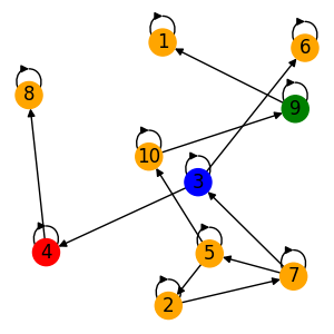
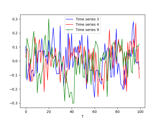
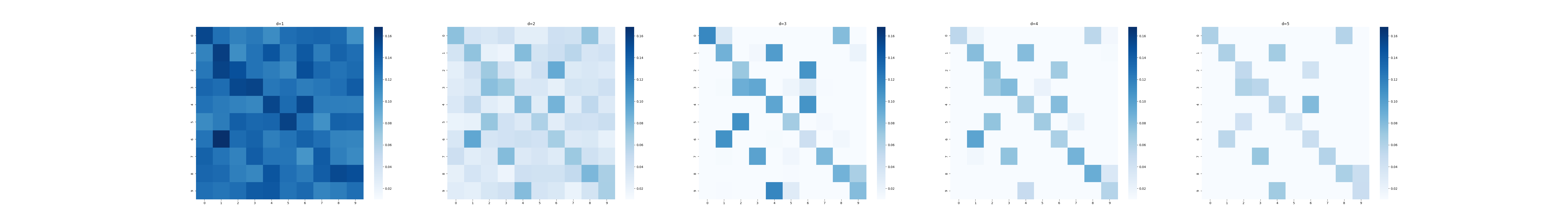
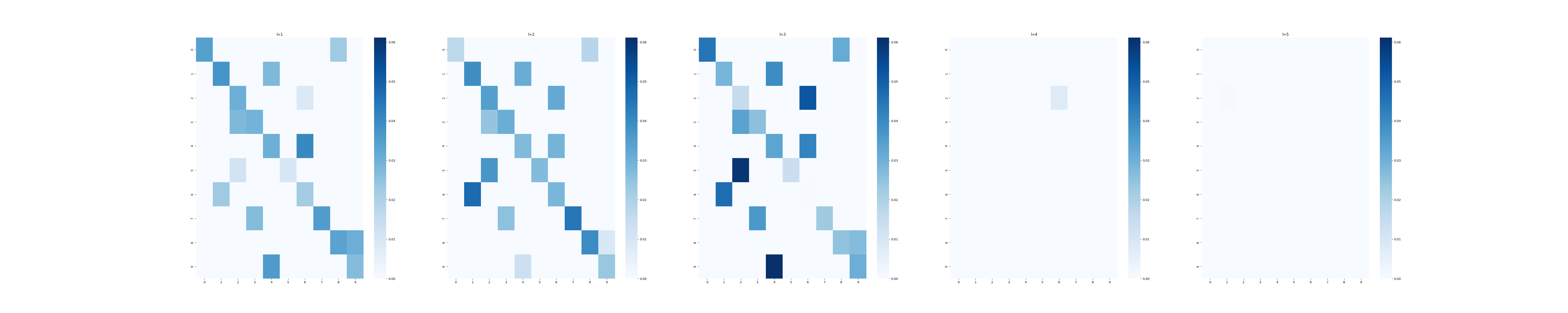
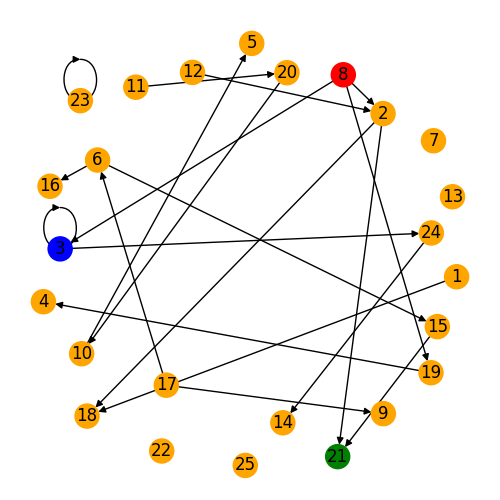
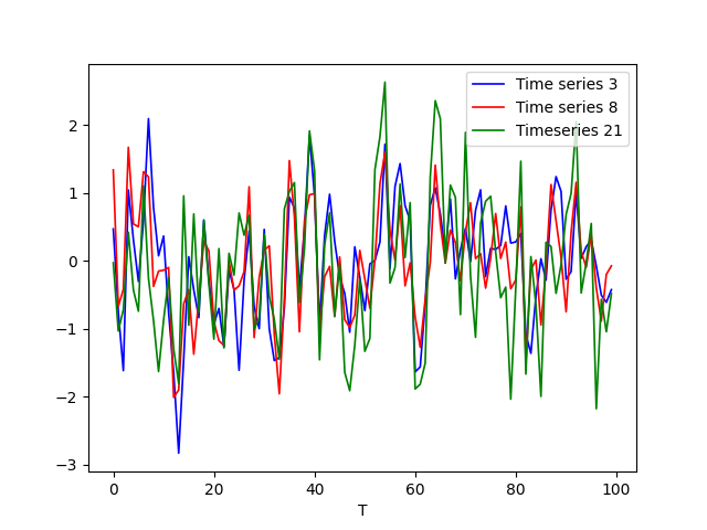
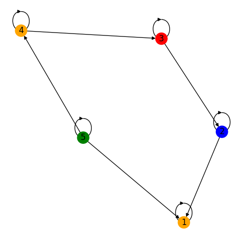
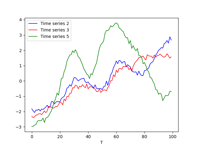
To qualitatively visualize the sparsity pattern recovered under the three lasso penalties, we apply our framework to data generated from a sparse VAR(3) model with , presented in [28]. Here, each time series depends on itself together with one other randomly selected time series among the remaining ones, and when time series depends on time series , for , while all the other lag entries are zero. Thus, this setting corresponds to the ground truth of . The ground truth causal graph and three selected time series are depicted in Figure 2. Time series and exhibit a causal relationship, while neither is causally linked to the time series . We collect sample points per time series for analysis.
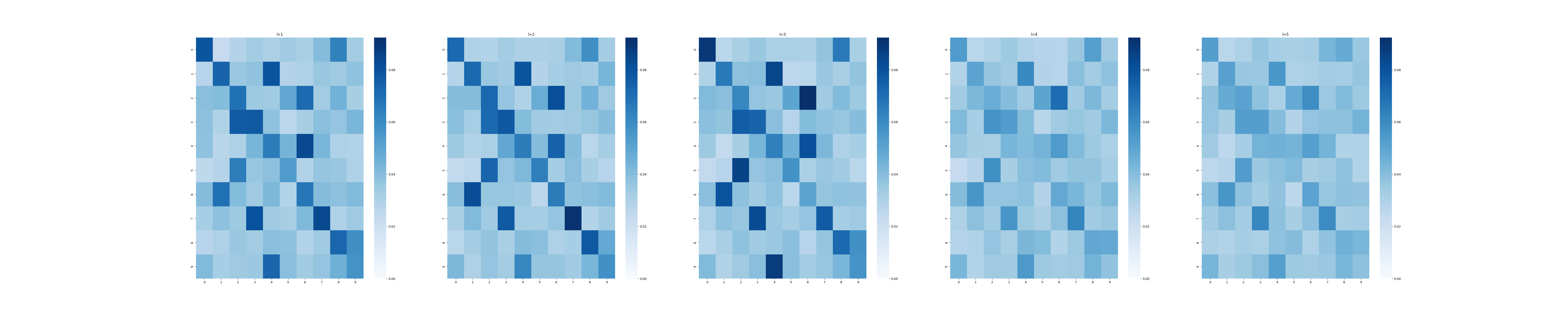
Because the data already follows linear dynamics, the nonlinear activation in each hidden layer was omitted. For causal model discovery, we set the learning rate , the number of hidden layers in lifting and projection networks as 2 with , the scaling-up factor of each dimension during lifting as , batch size , and the upper bound to lag . was chosen for the ulg- and ilg-lassos as an experimentally determined based penalty factor, while was used for the hlg-lasso, which again is the corresponding best value determined experimentally. The entries of the lag matrices are shown as heat-maps in Figure 3, where each entry is the norm of the entries in the lifted-version (all of which belong to a single group).
Taking a closer look at the captured blocks, i.e., for which for a suitable threshold value of epsilon (chosen experimentally), it can be seen in the cases of ilg- and hlg-lassos that if is shrunk to zero for some , then is also shrunk to zero. ilg- and hlg-lassos have different stopping epochs: vs , which implies ilg-lasso converges faster than hlg-lasso. On the other hand, while ulg-lasso converges just as fast as ilg-lasso: iterations, it cannot accurately match the right value of (as noted above, it runs the risk of treating the distant lag terms that may be absent in the ground truth the same as the near ones that are actually present in the ground truth). Based on these comparative observations of the three group lassos, moving forward, we have chosen to apply the NKDCD computations only for ilg- and hlg-lasso (both of which outperform ulg-lasso).
4 Results for Practical Applications
Our study demonstrates the performance of our novel NKDCD approach in inferring Granger causality (GC) and underlying dynamics from both synthetic and practically applicable datasets. We conduct experiments on financial data [39], Lorenz-96 model data [40], fMRI brain-imaging model data [39], and DREAM3 genetic data [42], sourced from various existing studies.
The results indicate that our NKDCD approach effectively discovers the underlying GC dependencies and nonlinear dynamics across various datasets. Key components of our model include a lifting encoder comprising multilayer perceptron (MLP) with hidden layers, GC weight matrices, and a projection decoder, another MLP with hidden layers. Each node in the encoder and decoder MLP has an activation function of a leakyReLU. We explore different hyperparameters, such as the learning rate () varied over ], and the sparsity weight () varied over . See Table I for a complete list of the hyperparameters chosen experimentally that we use in analyzing the application datasets. We set a convergence criterion as the average loss per time series being less than the threshold of and is no longer decreasing. The performance metrics are based on the area under the ROC curve (AUROC) and the area under the Precision-Recall curve (AUPR). We compare our results against linear VARs with hlg- and ilg-lasso for sparsity as formulated in Eqs. (2.1), (11), and (12) for baseline comparison, as well as the state-of-art results available in literature, including component-wise MLP (cMLP)/LSTM (cLSTM) as reported in [28], to demonstrate the gain resulting from the proposed NKDCD approach over the state-of-art. In our results, the weights corresponding to lag matrices, if they are small compared to a threshold (decided case-by-case for optimal result), are viewed zero to infer GC. Our NKDCD approach shows promising results, outperforming the ones reported in the literature.
| Finance | Lorenz-96 | fMRI | Dream3 | Dream3 | |
|---|---|---|---|---|---|
| (EC1,EC2,Y1) | (Y2,Y3) | ||||
| batch |
4.1 Finance Data
The simulated finance dataset utilized in our study originates from research reported in [39] and is publicly available on GitHub. This dataset is fitted to the Fama-French Three-Factors Model [46], a framework that characterizes stock returns against three factors: volatility, size, and value. For our experiments, we specifically utilize dataset 20-1, which comprises a -day observation period across stocks. In [39], the causal relationships among the time series present in this dataset evolve according to linear dynamics, and is within 1-3. The ground truth interdependency is provided in Figure 4a and a sample of three selected time series elements is depicted in 4b, where the causal relationship between time series and is evident. At the same time, neither has a causal connection with the time series . In this analysis, we set the maximum lag () to , and since the data already follows linear dynamics, the nonlinear activation (namely, leakyReLU) is omitted within the hidden layers.
| Dataset | 20-1 | |
|---|---|---|
| Metrics | AUROC | AUPR |
| NKDCD+Eq. 12 | ||
| NKDCD+Eq. 11 | ||
| VAR+Eq. 10 | ||
| VAR+Eq. 11 | ||
The performance metrics are reported as the mean across five initializations with a confidence interval. Results from our experiments on this finance dataset are summarized in Table II. The AUROC and AUPR for the VAR model with the ulg- and hlg-lasso penalties are both and , respectively. Our method performs just as well as the traditional VAR by giving AUROC and AUPR of and for the ilg-lasso penalty and and respectively for the hlg-lasso counterpart, showing that Koopman lifting preserves the causal relationship among the time series elements. These results demonstrate the effectiveness of our approach in uncovering the causal relationships and the underlying dynamics within the financial data having the 3-Factors linear model.
4.2 Lorenz-96 Model with Nonlinear Dynamics
The Lorenz-96 model, introduced in [40], serves as a valuable tool for studying essential aspects of chaos theory, predictability, and the behavior of complex nonlinear interdependent dynamics. It provides a simplified yet insightful representation of the atmospheric dynamics, making it widely used in atmospheric science and related fields. The continuous dynamics in a Lorenz-96 model is defined for as follows:
| (21) |
along with the following boundary correspondences:
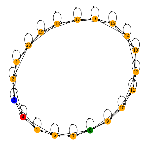
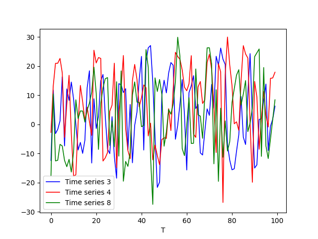
where is a forcing constant that determines the level of chaos, and is the dimension. For comparison with recent work, we utilized publicly available data of a Lorenz-96 model, described by Eq. 21 on GitHub, supplied by [28]. For our analysis, we chose and a sampling rate of for obtaining a discrete-time time series. The ground truth causal graph and three selected time series for are depicted in Figure 5. Notably, time series and exhibit a causal relationship, while neither is causally linked to time series .
| NKDCD+Eq. 12 | ||||||
|---|---|---|---|---|---|---|
| NKDCD+Eq. 11 | ||||||
| cMLP | ||||||
| cLSTM | ||||||
| VAR+Eq. 10 | ||||||
| VAR+Eq. 11 | ||||||
We conduct simulations for and , as specified in Table III, where our objective is to compare the performance of the NKDCD approach against other state-of-art methods in literature, including component-wise MLP (cMLP)/LSTM (cLSTM) as reported in [28], and the standard linear VAR method. The performance metrics are reported as the mean across five initializations with a confidence interval.
The results, summarized in Table III, reveal a tradeoff between accuracy and length of observation as increases. Despite challenges posed by shorter data lengths and higher chaos levels, NKDCD demonstrates superior performance over alternative methods in most scenarios, except for a single scenario when the data length is small (), and chaos is greater (), it is cMLP performs the best with NKDCD being the second best. At , the AUROCs for the VAR with ulg- and hlg-lassos are both , and respectively. The AUROCs for cMLP are reported to be , and respectively, while those for cLSTM are , and respectively. NKDCD with ilg-lasso penalty gives AUROC of , and while its counterpart with hlg-lasso is , and respectively. When F is increased to , for the AUROCs for the VAR with ulg-lasso are , , and , and with hlg-lasso are , , and respectively. The AUROCs for cMLP are reported to be , , and , while those of cLSTM are , , and respectively. NKDCD with ilg-lasso penalty gives AUROC of , , and while its counterpart with hlg-lasso is , , and respectively.
4.3 fMRI Data with Nonlinear Dynamics
Another benchmark, functional magnetic resonance imaging (fMRI), contains realistic, simulated Blood-oxygen-level dependent (BOLD) datasets for different underlying brain networks [41]. BOLD fMRI measures the neural activity of different regions of interest in the brain based on the changes in blood flow. Each region (i.e., a node in the brain network) has its associated time series of electrical excitation. All time series have an external input, white noise, and are fed through a nonlinear model [47]. All datasets are also made available on GitHub. Brain network has a dataset of size that corresponds to one of the brain networks. Its ground truth causal graph and three selected time series are depicted in Figure 6, in which time series and exhibit a causal relationship, while neither is causally linked to time series .
| Dataset | Brain network 20 | |
|---|---|---|
| Metrics | AUROC | AUPR |
| NKDCD+Eq. 12 | ||
| NKDCD+Eq. 11 | ||
| VAR+Eq. 10 | ||
| VAR+Eq. 11 | ||
The performance metrics are reported as the mean across five initializations with a confidence interval. The results, summarized in Table IV, show that our formulation is promising and can be utilized in realistic datasets. The AUROC and AUPR for the standard VAR method using ulg- and hlg-lasso penalties are and , respectively. Our method outperforms the VARs by having AUROC and AUPR of and for the ilg-lasso penalty and and respectively for the hlg- counterpart.
4.4 Dream3 Genetic Data with Nonlinear Dynamics
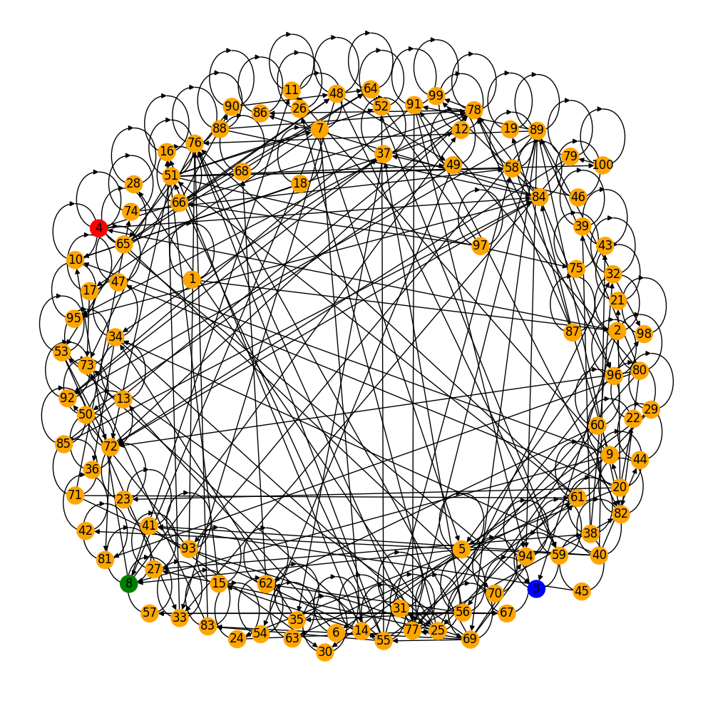
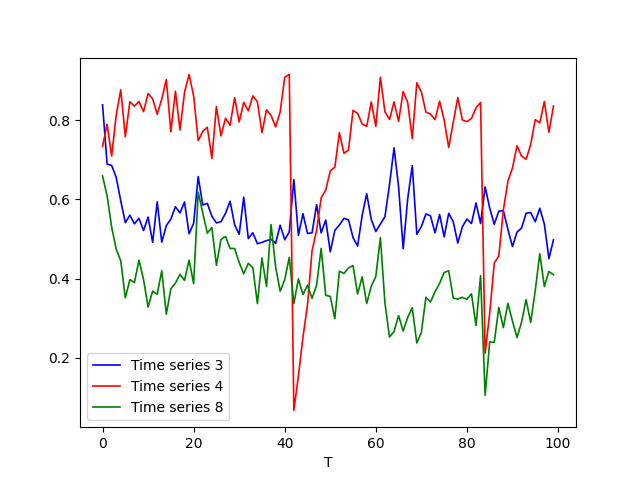
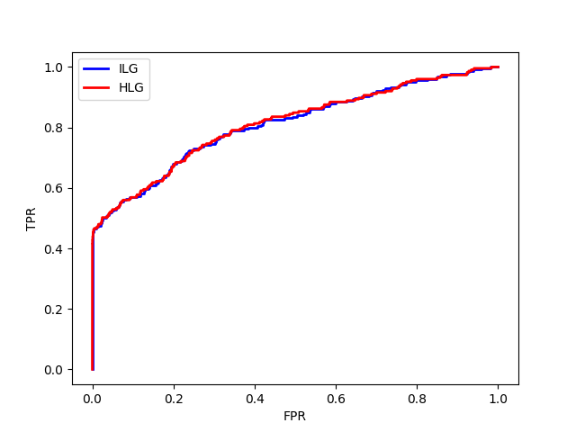
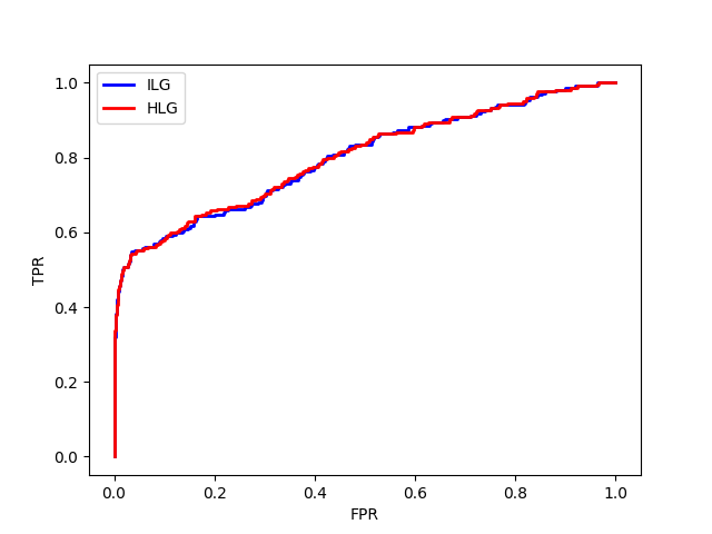
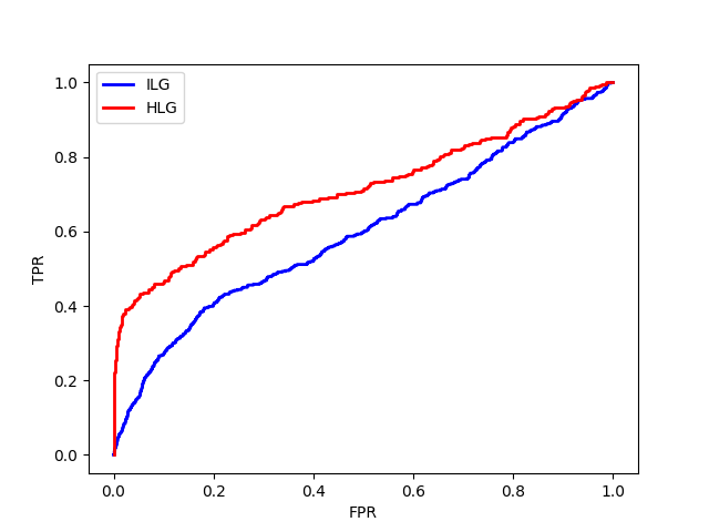
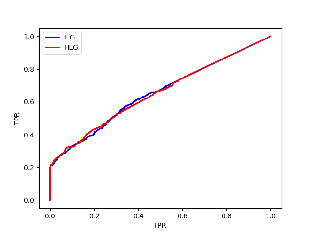
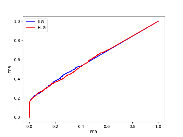
DREAM3 challenge dataset [42] provides a rigorous benchmark for comparing GC detection methods for gene regulatory networks [48, 49, 28]. The data are synthetically generated to mimic continuous gene expression and regulation dynamics, incorporating multiple unobserved hidden factors. The DREAM3 challenge comprises distinct simulated datasets, each associated with different ground truth GC dependencies. Specifically, there are two datasets based on E.coli (EC 1-2) and three datasets based on Yeast (Y 1-3). In each dataset, there are time series, with replicates sampled at time points, resulting in a times series data of size . This setup presents a significant challenge due to the limited amounts of data relative to the complexity of the networks and underlying dynamic interactions, as shown in Figure 7a, whereas selected time series elements from a single replicate of the Y1 dataset are shown in Figure 7b. This snapshot provides insight into the intricacies of the gene expression dynamics encapsulated within the dataset, offering a stage for our GC estimation efforts. In this simulation, the ADAM [50] with parameters and , was used to initially update the learnable parameters in place of the ordinary gradient descent, followed by the proximal gradient descent was used to sparsify the lag matrices . We applied our results to all five data sets. Results for AUROC are visualized in Figure 8a and for AUPR in Figure 8b. The ROC plots for both the ilg- and hlg-lassos are shown in Figure 9.
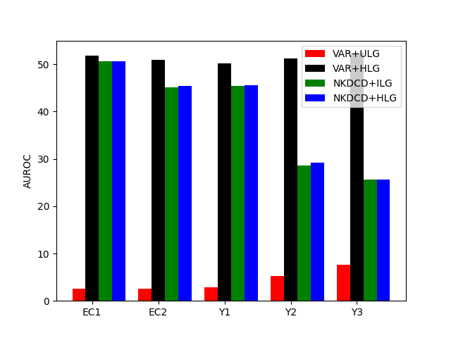
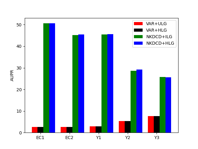
We compared our results based on the bar plots in the recent work reported in [28] in Table V. For the EC1 dataset, the AUROC values for the standrad VAR with ulg-lasso and with hlg-lasso, cMLP, cLSTM, NKDCD with ilg-lasso, and with hlg-lasso respectively are ,, , , and their corresponding AUPRs are , , , , , , respectively. Following the same pattern for the EC2 dataset, the AUROCs are , ,, , , and their corresponding AUPRs are , , , , , , respectively. The performance of the Y1 dataset for AUROCs are , ,, , , and their corresponding AUPRs are , , , , , , respectively. The Y2 dataset yields AUROCs are as, , ,, , , and their corresponding AUPRs as, , , , , , , respectively. The Y3 Dataset gives AUROCs as, , ,, , , and their corresponding AUPRs as, , , , , , , respectively. Results suggest that the dynamics for Y 1-3 may be more complex than that for EC 1-2. In all cases, our results outperform the existing linear and nonlinear methods.
5 Conclusion
We have introduced the NeuroKoopman Dynamic Causal Discovery (NKDCD) framework, which leverages a Koopman-inspired regularized deep neural network autoencoder architecture for the inference of nonlinear Granger causality and underlying dynamics in observed multivariate time series data. This framework enables the learning of underlying dynamics and their interdependencies through sparse nonlinear regressive models. By employing a data-driven NN-based basis function for lifting the NAR dependency for a linear Koopman embedding and next for learning a linear vector autoregressive model in the lifted domain, we infer Granger causality and the underlying dynamics. We employ structured group-level sparsity-inducing penalties that preserve the structure of interdependencies of the original variables, ensuring reliable model learning. Validation through simulations on various application datasets shows that our NKDCD outperforms the state-of-the-art results from recent literature.
Bibliography & References Cited
- [1] R. Guo, L. Cheng, J. Li, P. R. Hahn, and H. Liu, “A survey of learning causality with data: Problems and methods,” ACM Computing Surveys (CSUR), vol. 53, no. 4, pp. 1–37, 2020.
- [2] C. W. Granger, “Investigating causal relations by econometric models and cross-spectral methods,” Econometrica: Journal of the Econometric Society, pp. 424–438, 1969.
- [3] H. Lütkepohl, New Introduction to Multiple Time Series Analysis. Springer Science & Business Media, 2005.
- [4] Y. Hong, Y. Liu, and S. Wang, “Granger causality in risk and detection of extreme risk spillover between financial markets,” Journal of Econometrics, vol. 150, no. 2, pp. 271–287, 2009.
- [5] A. T. Reid, D. B. Headley, R. D. Mill, R. Sanchez-Romero, L. Q. Uddin, D. Marinazzo, D. J. Lurie, P. A. Valdés-Sosa, S. J. Hanson, B. B. Biswal et al., “Advancing functional connectivity research from association to causation,” Nature neuroscience, vol. 22, no. 11, pp. 1751–1760, 2019.
- [6] T. J. Mosedale, D. B. Stephenson, M. Collins, and T. C. Mills, “Granger causality of coupled climate processes: Ocean feedback on the north atlantic oscillation,” Journal of climate, vol. 19, no. 7, pp. 1182–1194, 2006.
- [7] S. Z. Chiou-Wei, C.-F. Chen, and Z. Zhu, “Economic growth and energy consumption revisited—evidence from linear and nonlinear granger causality,” Energy economics, vol. 30, no. 6, pp. 3063–3076, 2008.
- [8] P. A. Stokes and P. L. Purdon, “A study of problems encountered in Granger causality analysis from a neuroscience perspective,” Proceedings of the National Academy of Sciences, vol. 114, no. 34, pp. E7063–E7072, 2017.
- [9] A. Sheikhattar, S. Miran, J. Liu, J. B. Fritz, S. A. Shamma, P. O. Kanold, and B. Babadi, “Extracting neuronal functional network dynamics via adaptive Granger causality analysis,” Proceedings of the National Academy of Sciences, vol. 115, no. 17, pp. E3869–E3878, 2018.
- [10] A. Fujita, P. Severino, J. R. Sato, and S. Miyano, “Granger causality in systems biology: modeling gene networks in time series microarray data using vector autoregressive models,” in Brazilian Symposium on Bioinformatics. Springer, 2010, pp. 13–24.
- [11] A. C. Lozano, N. Abe, Y. Liu, and S. Rosset, “Grouped graphical granger modeling methods for temporal causal modeling,” in Proceedings of the 15th ACM SIGKDD International Conference on Knowledge Discovery and Data Mining. ACM, 2009, pp. 577–586.
- [12] C. A. Sims, “Money, income, and causality,” The American economic review, vol. 62, no. 4, pp. 540–552, 1972.
- [13] G. Chamberlain, “The general equivalence of granger and sims causality,” Econometrica: Journal of the Econometric Society, pp. 569–581, 1982.
- [14] J. B. Cromwell, Multivariate tests for time series models. Sage, 1994, no. 100.
- [15] R. Tibshirani, “Regression shrinkage and selection via the lasso,” Journal of the Royal Statistical Society: Series B (Methodological), vol. 58, no. 1, pp. 267–288, 1996.
- [16] M. Yuan and Y. Lin, “Model selection and estimation in regression with grouped variables,” Journal of the Royal Statistical Society: Series B (Statistical Methodology), vol. 68, no. 1, pp. 49–67, 2006.
- [17] W. B. Nicholson, J. Bien, and D. S. Matteson, “Hierarchical vector autoregression,” arXiv preprint arXiv:1412.5250, 2014.
- [18] A. Shojaie and G. Michailidis, “Discovering graphical Granger causality using the truncating lasso penalty,” Bioinformatics, vol. 26, no. 18, pp. i517–i523, 2010.
- [19] T. Teräsvirta, D. Tjøstheim, C. W. J. Granger et al., Modelling Nonlinear Economic Time Series. Oxford University Press Oxford, 2010.
- [20] B. Lusch, P. D. Maia, and J. N. Kutz, “Inferring connectivity in networked dynamical systems: Challenges using Granger causality,” Physical Review E, vol. 94, no. 3, p. 032220, 2016.
- [21] R. Vicente, M. Wibral, M. Lindner, and G. Pipa, “Transfer entropy—a model-free measure of effective connectivity for the neurosciences,” Journal of Computational Neuroscience, vol. 30, no. 1, pp. 45–67, 2011.
- [22] P.-O. Amblard and O. J. Michel, “On directed information theory and Granger causality graphs,” Journal of Computational Neuroscience, vol. 30, no. 1, pp. 7–16, 2011.
- [23] J. Runge, J. Heitzig, V. Petoukhov, and J. Kurths, “Escaping the curse of dimensionality in estimating multivariate transfer entropy,” Physical Review Letters, vol. 108, no. 25, p. 258701, 2012.
- [24] M. Raissi, P. Perdikaris, and G. E. Karniadakis, “Multistep neural networks for data-driven discovery of nonlinear dynamical systems,” arXiv preprint arXiv:1801.01236, 2018.
- [25] Ö. Kişi, “River flow modeling using artificial neural networks,” Journal of Hydrologic Engineering, vol. 9, no. 1, pp. 60–63, 2004.
- [26] A. Graves, “Supervised sequence labelling,” in Supervised Sequence Labelling with Recurrent Neural Networks. Springer, 2012, pp. 5–13.
- [27] Y. Li, R. Yu, C. Shahabi, and Y. Liu, “Graph convolutional recurrent neural network: Data-driven traffic forecasting,” arXiv preprint arXiv:1707.01926, 2017.
- [28] A. Tank, I. Covert, N. Foti, A. Shojaie, and E. B. Fox, “Neural granger causality,” IEEE Transactions on Pattern Analysis and Machine Intelligence, vol. 44, no. 8, pp. 4267–4279, 2021.
- [29] B. O. Koopman, “Hamiltonian systems and transformation in hilbert space,” Proceedings of the National Academy of Sciences, vol. 17, no. 5, pp. 315–318, 1931.
- [30] M. O. Williams, I. G. Kevrekidis, and C. W. Rowley, “A data–driven approximation of the koopman operator: Extending dynamic mode decomposition,” Journal of Nonlinear Science, vol. 25, pp. 1307–1346, 2015.
- [31] P. J. Schmid, “Dynamic mode decomposition and its variants,” Annual Review of Fluid Mechanics, vol. 54, pp. 225–254, 2022.
- [32] M. Korda and I. Mezić, “Linear predictors for nonlinear dynamical systems: Koopman operator meets model predictive control,” Automatica, vol. 93, pp. 149–160, 2018.
- [33] S. Sinha and U. Vaidya, “On data-driven computation of information transfer for causal inference in discrete-time dynamical systems,” Journal of Nonlinear Science, vol. 30, no. 4, pp. 1651–1676, 2020.
- [34] R. Gunjal, S. S. Nayyer, S. Wagh, A. Stankovic, and N. Singh, “Granger causality for prediction in dynamic mode decomposition: Application to power systems,” Electric Power Systems Research, vol. 225, p. 109865, 2023. [Online]. Available: https://www.sciencedirect.com/science/article/pii/S0378779623007538
- [35] I. Goodfellow, Y. Bengio, and A. Courville, Deep learning. MIT press, 2016.
- [36] C. Wehmeyer and F. Noé, “Time-lagged autoencoders: Deep learning of slow collective variables for molecular kinetics,” The Journal of chemical physics, vol. 148, no. 24, 2018.
- [37] B. Lusch, J. N. Kutz, and S. L. Brunton, “Deep learning for universal linear embeddings of nonlinear dynamics,” Nature communications, vol. 9, no. 1, p. 4950, 2018.
- [38] R. R. Hossain, R. Adesunkanmi, and R. Kumar, “Data-driven linear koopman embedding for networked systems: Model-predictive grid control,” IEEE Systems Journal, 2023.
- [39] M. Nauta, D. Bucur, and C. Seifert, “Causal discovery with attention-based convolutional neural networks,” Machine Learning and Knowledge Extraction, vol. 1, no. 1, pp. 312–340, 2019.
- [40] E. N. Lorenz, “Predictability: A problem partly solved,” in Proc. Seminar on predictability, vol. 1, no. 1. Reading, 1996.
- [41] S. M. Smith, K. L. Miller, G. Salimi-Khorshidi, M. Webster, C. F. Beckmann, T. E. Nichols, J. D. Ramsey, and M. W. Woolrich, “Network modelling methods for fmri,” Neuroimage, vol. 54, no. 2, pp. 875–891, 2011.
- [42] R. J. Prill, D. Marbach, J. Saez-Rodriguez, P. K. Sorger, L. G. Alexopoulos, X. Xue, N. D. Clarke, G. Altan-Bonnet, and G. Stolovitzky, “Towards a rigorous assessment of systems biology models: the dream3 challenges,” PloS One, vol. 5, no. 2, p. e9202, 2010.
- [43] A. C. Lozano, N. Abe, Y. Liu, and S. Rosset, “Grouped graphical granger modeling for gene expression regulatory networks discovery,” Bioinformatics, vol. 25, no. 12, pp. i110–i118, 2009.
- [44] A. Tank, I. Covert, N. Foti, A. Shojaie, and E. Fox, “Neural granger causality,” arXiv preprint arXiv:1802.05842, 2018.
- [45] N. Parikh, S. Boyd et al., “Proximal algorithms,” Foundations and Trends in Optimization, vol. 1, no. 3, pp. 127–239, 2014.
- [46] E. F. Fama and K. R. French, “The cross-section of expected stock returns,” the Journal of Finance, vol. 47, no. 2, pp. 427–465, 1992.
- [47] R. B. Buxton, E. C. Wong, and L. R. Frank, “Dynamics of blood flow and oxygenation changes during brain activation: the balloon model,” Magnetic resonance in medicine, vol. 39, no. 6, pp. 855–864, 1998.
- [48] N. Lim, F. d’Alché Buc, C. Auliac, and G. Michailidis, “Operator-valued kernel-based vector autoregressive models for network inference,” Machine learning, vol. 99, pp. 489–513, 2015.
- [49] S. Lèbre, “Inferring dynamic genetic networks with low order independencies,” Statistical applications in genetics and molecular biology, vol. 8, no. 1, 2009.
- [50] D. P. Kingma and J. Ba, “Adam: A method for stochastic optimization,” arXiv preprint arXiv:1412.6980, 2014.
![[Uncaptioned image]](/html/2404.16326/assets/figures/rahma_ieee.jpg) |
Rahmat Adesunkanmi is a Ph.D. student at the Department of Electrical and Computer Engineering, Iowa State University, Ames, USA. She received her B.S. degree from the University of Ibadan, Nigeria, in 2015 and subsequently her master’s degree from Iowa State University. Her research interests include noise-robust Machine learning techniques and Time-series analysis. She is an active member of the Graduate Society for Women Engineers. |
| Balaji Sesha Srikanth Pokuri received the B.Tech degree in electrical engineering from Indian Institute of Technology, Roorkee, India, in 2017. He is currently working toward the Ph.D. degree in electrical engineering with the Department of Electrical and Computer Engineering, Iowa State University, Ames, IA, USA. He worked as a Quantitative Analyst in eFX Trading business of HSBC Global Markets, from 2017 to 2021. His current research includes data-driven modeling, control, optimization, and artificial-intelligence-based approaches for precision agriculture. |
![[Uncaptioned image]](/html/2404.16326/assets/figures/ratnesh_ieee.jpg) |
Ratnesh Kumar is a Palmer Professor at the Department of Electrical and Computer Engineering, Iowa State University, where he directs the ESSeNCE (Embedded Software, Sensors, Networks, Cyberphysical, and Energy) Lab. Previously, he held a faculty position at the University of Kentucky and various visiting positions with the University of Maryland (College Park), the Applied Research Laboratory at the Pennsylvania State University (State College), NASA Ames, the Idaho National Laboratory, the United Technologies Research Center, and the Air Force Research Laboratory. He received a B. Tech. degree in Electrical Engineering from IIT Kanpur, India, in 1987 and the M.S. and Ph.D. degrees in Electrical and Computer Engineering from the University of Texas at Austin in 1989 and 1991 respectively. Ratnesh is a Fellow of IEEE, also a Fellow of AAAS, and was a Distinguished Lecturer of the IEEE Control Systems Society. He is a recipient of D. R. Boylan Eminent Faculty Award for Research and Award for Outstanding Achievement in Research from Iowa State University, and also the Distinguished Alumni Award from IIT Kanpur. Ratnesh received Gold Medals for the Best EE Undergrad, the Best All Rounder, and the Best EE Project from IIT Kanpur, and the Best Dissertation Award from UT Austin, the Best Paper Award from the IEEE Transactions on Automation Science and Engineering, and has been Keynote Speaker and paper award recipient from multiple conferences. He is or has been an editor of several journals (including of IEEE, SIAM, ACM, Springer, IET, MDPI). |