MaGGIe: Masked Guided Gradual Human Instance Matting

Abstract

Human matting is a foundation task in image and video processing where human foreground pixels are extracted from the input. Prior works either improve the accuracy by additional guidance or improve the temporal consistency of a single instance across frames. We propose a new framework MaGGIe, Masked Guided Gradual Human Instance Matting, which predicts alpha mattes progressively for each human instances while maintaining the computational cost, precision, and consistency. Our method leverages modern architectures, including transformer attention and sparse convolution, to output all instance mattes simultaneously without exploding memory and latency. Although keeping constant inference costs in the multiple-instance scenario, our framework achieves robust and versatile performance on our proposed synthesized benchmarks. With the higher quality image and video matting benchmarks, the novel multi-instance synthesis approach from publicly available sources is introduced to increase the generalization of models in real-world scenarios. Our code and datasets are available at https://maggie-matt.github.io.

1 Introduction

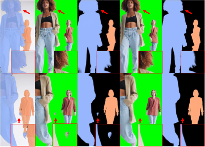
Guidance masks

$\underbrace{\hskip 93.89418pt}_{\hbox{\pagecolor{white}~{}~{}InstMatt~{}\cite[cite]{[\@@bibref{Number}{sun2022instmatt}{}{}]}~{}~{}}}$

$\underbrace{\hskip 93.89418pt}_{\hbox{\pagecolor{white}~{}~{}MaGGIe (ours)~{}~{}}}$

Figure 1: Our MaGGIe delivers precise and temporally consistent alpha mattes. It adeptly preserves intricate details and demonstrates robustness against noise in instance guidance masks by effectively utilizing information from adjacent frames. Red arrows highlight the areas of detailed zoom-in. (Optimally viewed in color and digital zoom in).

In image matting, a trivial solution is to predict the pixel transparency - alpha matte $\alpha\in[0,1]$ for precise background removal. Considering a saliency image $I$ with two main components, foreground $F$ and background $B$, the image $I$ is expressed as $I=\alpha F+(1-\alpha)B$. Because of the ambiguity in detecting the foreground region, for example, whether a person’s belongings are a part of the human foreground or not, many methods [16, 31, 37, 11] leverage additional guidance, typically trimaps, defining foreground, background, and unknown or transition regions. However, creating trimaps, especially for videos, is resource-intensive. Alternative binary masks [56, 39] are simpler to obtain by human drawings or off-the-shelf segmentation models while offering greater flexibility without hardly constraint output values of regions as trimaps. Our work focuses but is not limited to human matting because of the higher number of available academic datasets and user demand in many applications [2, 12, 44, 1, 15] compared to other objects.

When working with video input, the problem of creating trimap guidance is often resolved by guidance propagation [45, 17] where the main idea coming from video object segmentation [38, 8]. However, the performance of trimap propagation degrades when video length grows. The failed trimap predictions, which miss some natures like the alignment between foreground-unknown-background regions, lead to incorrect alpha mattes. We observe that using binary masks for each frame gives more robust results. However, the consistency between the frame’s output is still important for any video matting approach. For example, holes appearing in a random frame because of wrong guidance should be corrected by consecutive frames. Many works [34, 45, 17, 32, 53] constrain the temporal consistency at feature maps between frames. Since the alpha matte values are very sensitive, feature-level aggregation is not an absolute guarantee of the problem. Some methods [21, 50] in video segmentation and matting compute the incoherent regions to update values across frames. We propose a temporal consistency module that works in both feature and output spaces to produce consistent alpha mattes.

Instance matting [49] is an extension of the matting problem where there exists multiple $\alpha_{i},i\in{0..N}$, and each belongs to one foreground instance. This problem creates another constraint for each spatial location $(x,y)$ value such that $\sum_{i}\alpha_{i}(x,y)=1$. The main prior work InstMatt [49] handles the multi-instance images by predicting each alpha matte separately from binary guided masks before the instance refinement at the end. Although this approach produces impressive results in both synthesized and natural image benchmarks, the efficiency and accuracy of this model are unexplored in video processing. The separated prediction for each instance yields inefficiency in the architecture, which makes it costly to adapt to video input. Another concurrent work [30] with ours extends the InstMatt to process video input, but the complexity and efficiency of the network are unexplored. Fig. 1 illustrates the comparison between our MaGGIe and InstMatt when working with video. Our work improves not only the accuracy but also the consistency between frames when errors occur in guidance.

Besides the temporal consistency, when extending the instance matting to videos containing a large number of frames and instances, the careful network design to prevent the explosion in the computational cost is also a key challenge. In this work, we propose several adjustments to the popular mask-guided progressive refinement architecture [56]. Firstly, by using the mask guidance embedding inspired by AOT [55], the input size reduces to a constant number of channels. Secondly, with the advancement of transformer attention in various vision tasks [42, 41, 40], we inherit the query-based instance segmentation [23, 19, 7] to predict instance mattes in one forward pass instead of separated estimation. It also replaces the complex refinement in previous work with the interaction between instances by attention mechanism. To save the high cost of transformer attention, we only perform multi-instance prediction at the coarse level and adapt the progressive refinement at multiple scales [56, 18]. However, using full convolution for the refinement as previous works are inefficient as less than 10% of values are updated at each scale, which is also mentioned in [50]. The replacement of sparse convolution [36] saves the inference cost significantly, keeping the constant complexity of the algorithm since only interested locations are refined. Nevertheless, the lack of information at a larger scale when using sparse convolution can cause a dominance problem, which leads to the higher-scale prediction copying the lower outputs without adding fine-grained details. We propose an instance guidance method to help the coarser prediction guide but not contribute to the finer alpha matte.

In addition to the framework design, we propose a new training video dataset and benchmarks for instance-awareness matting. Besides the new large-scale high-quality synthesized image instance matting, an extension of the current instance image matting benchmark adds more robustness with different guidance quality. For video input, our synthesized training and benchmark are constructed from various public instance-agnostic datasets with three levels of difficulty.

In summary, our contributions include:

• A highly efficient instance matting framework with mask guidance that has all instances interacting and processed in a single forward pass.

• A novel approach that considers feature-matte levels to maintain matte temporal consistency in videos.

• Diverse training datasets and robust benchmarks for image and video instance matting that bridge the gap between synthesized and natural cases.

2 Related Works

There are many ways to categorize matting methods, here we revise previous works based on their primary input types. The brief comparison of others and our MaGGIe is shown in Table 2.

Image Matting. Traditional matting methods [25, 24, 4] rely on color sampling to estimate foreground and background, often resulting in noisy outcomes due to limited high-level object features. Advanced deep learning-based methods [9, 46, 54, 47, 37, 31, 11] have significantly improved results by integrating image and trimap inputs or focusing on high-level and detailed feature learning. However, these methods often struggle with trimap inaccuracies and assume single-object scenarios. Recent approaches [22, 5, 6] require only image inputs but face challenges with multiple salient objects. MGM [56] and its extension MGM-in-the-wild [39] introduce binary mask-based matting, addressing multi-salient object issues and reducing trimap dependency. InstMatt [49] further customizes this approach for multi-instance scenarios with a complex refinement algorithm. Our work extends these developments, focusing on efficient, end-to-end instance matting with binary mask guidance. Image matting also benefits from diverse datasets [54, 27, 26, 29, 22, 33, 50], supplemented by background augmentation from sources like BG20K [29] or COCO [35]. Our work also leverages currently available datasets to concretize a robust benchmark for human-masked guided instance matting.

Video Matting. Temporal consistency is a key challenge in video matting. Trimap-propagation methods [48, 45, 17] and background knowledge-based approaches like BGMv2 [33] aim to reduce trimap dependency. Recent techniques [34, 32, 53, 57, 28] incorporate Conv-GRU, attention memory matching, or transformer-based architectures for temporal feature aggregation. SparseMat [50] uniquely focuses on fusing outputs for consistency. Our approach builds on these foundations, combining feature and output fusion for enhanced temporal consistency in alpha maps. There is a lack of video matting datasets due to the difficulty in data collecting. VideoMatte240K [33] and VM108 [57] focus on composited videos, while CRGNN [52] is the only offering natural videos for human matting. To address the gap in instance-aware video matting datasets, we propose adapting existing public datasets for training and evaluation, particularly for human subjects.

Table 1: Comparing MaGGIe with previous works in image and video matting. Our work is the first instance-aware framework producing alpha matte from a binary mask with both feature and output temporal consistency in constant processing time.

Method	Avenue	Guidance	Instance
-awareness	Temp. aggre.		Time
complexity
				Feat.	Matte.
MGM [56, 39]	CVPR21+23	Mask				$O(n)$
InstMatt [49]	CVPR22	Mask	✓			$O(n)$
TCVOM [57]	MM21	-	-	✓		-
OTVM [45]	ECCV22	1st trimap		✓		$O(n)$
FTP-VM [17]	CVPR23	1st trimap		✓		$O(n)$
SparseMatt [50]	CVPR23	No			✓	$O(n)$
MaGGIe	-	Mask	✓	✓	✓	$\approx O(1)$

3 MaGGIe

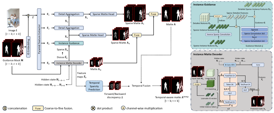
Figure 2: Overall pipeline of MaGGIe. This framework processes frame sequences $\mathbf{I}$ and instance masks $\mathbf{M}$ to generate per-instance alpha mattes $\mathbf{A}^{\prime}$ for each frame. It employs progressive refinement and sparse convolutions for accurate mattes in multi-instance scenarios, optimizing computational efficiency. The subfigures on the right illustrate the Instance Matte Decoder and the Instance Guidance, where we use mask guidance to predict coarse instance mattes and guide detail refinement by deep features, respectively. (Optimal in color and zoomed view).

We introduce our efficient instance matting framework guided by instance binary masks, structured into two parts. The first Sec. 3.1 details our novel architecture to maintain accuracy and efficiency. The second Sec. 3.2 describes our approach for ensuring temporal consistency across frames in video processing.

3.1 Efficient Masked Guided Instance Matting

Our framework, depicted in Fig. 2, processes images or video frames $\mathbf{I}\in[0,255]^{T\times 3\times H\times W}$ with corresponding binary instance guidance masks $\mathbf{M}\in\{0,1\}^{T\times N\times H\times W}$, and then predicts alpha mattes $\mathbf{A}\in[0,1]^{T\times N\times H\times W}$ for each instance per frame. Here, $T,N,H,W$ represent the number of frames, instances, and input resolution, respectively. Each spatial-temporal location $(x,y,t)$ in $\mathbf{M}$ is a one-hot vector $\{0,1\}^{N}$ highlighting the instance it belongs to. The pipeline comprises five stages: (1) Input construction; (2) Image features extraction; (3) Coarse instance alpha mattes prediction; (4) Progressive detail refinement; and (5) Coarse-to-fine fusion.

Input Construction. The input $\mathbf{I}^{\prime}\in\mathbb{R}^{T\times(3+C_{e})\times H\times W}$ to our model is the concatenation of input image $\mathbf{I}^{\prime}$ and guidance embedding $\mathbf{E}\in\mathbb{R}^{T\times C_{e}\times H\times W}$ constructed from $\mathbf{M}$ by ID Embedding layer [55]. More details about transforming $\mathbf{M}$ to $\mathbf{E}$ are in the supplementary material.

Image Features Extraction. We extract features map $\mathbf{F}_{s}\in\mathbb{R}^{T\times C_{s}\times H/s\times W/s}$ from $\mathbf{I}^{\prime}$ by feature-pyramid networks. As shown in the left part of Fig. 2, there are four scales $s={1,2,4,8}$ for our coarse-to-fine matting pipeline.

Coarse instance alpha mattes prediction. Our MaGGIe adopts transformer-style attention to predict instance mattes at the coarsest features $\mathbf{F}_{8}$. We revisit the scaled dot-product attention mechanism in Transformers [51]. Given queries $\mathbf{Q}\in\mathbb{R}^{L\times C}$, keys $\mathbf{K}\in\mathbb{R}^{S\times C}$, and values $\mathbf{V}\in\mathbb{R}^{S\times C}$, the scaled dot-product attention is defined as:

$$\text{Attention}(\mathbf{Q},\mathbf{K},\mathbf{V})=\text{softmax}\left(\frac{\mathbf{Q}\mathbf{K}^{\top}}{\sqrt{C}}\right)\mathbf{V}.$$ (1)

In cross-attention (CA), $\mathbf{Q}$ and $(\mathbf{K},\mathbf{V})$ originate from different sources, whereas in self-attention (SA), they share similar information.

In our Instance Matte Decoder, the organization of CA and SA blocks inspired by SAM [23] is depicted in the bottom right of Fig. 2. The downscaled guidance masks $\mathbf{M}_{8}$ also participate as the additional embedding for image features in attention procedures. The coarse alpha matte $\mathbf{A}_{8}$ is computed as the dot product between instance tokens $\mathbf{T}=\{\mathbf{T}_{i}|1\leq i\leq N\}\in\mathbb{R}^{N\times C_{8}}$ and enriched feature map $\bar{\mathbf{F}}_{8}$ with a sigmoid activation applied. Those components are used in the following steps of matte detail refinement.

Progressive Detail Refinement. From the coarse instance alpha matte, we leverage the Progressive Refinement [56] to improve the details at uncertain locations $\mathbf{U}=\{u_{p}=(x,y,t,i)|0<\mathbf{A}_{8}(u_{p})<1\}\in\mathbb{N}^{P\times 4}$ with some highly efficient modifications. It is mandatory to transform enriched dense features $\bar{\mathbf{F}}_{8}$ to instance-specific features $\mathbf{X}_{8}$ for the instance-wise refinement. However, to save memory and computational costs, only transformed features at uncertainty $\mathbf{U}$ are computed as:

$$\mathbf{X}_{8}(x,y,t,i)=\text{MLP}(\mathbf{\bar{F}}_{8}(x,y,t)\times\mathbf{T}_{i}).$$ (2)

To combine the coarser instance-specific sparse features $\mathbf{X}_{8}$ with the finer image features $\mathbf{F}_{4}$, we propose the Instance Guidance (IG) module. As described in the top right of Fig. 2, this module firstly increases the spatial scale of $\mathbf{X}_{8}$ to have $\mathbf{X}^{\prime}_{4}$ by an inverse sparse convolution. For each entry $p$, we compute a guidance score $\mathbf{G}\in[0,1]^{C_{4}}$, which is then channel-wise multiplied with $\mathbf{F}_{4}$ to produce detailed sparse instance-specific features $\mathbf{X}_{4}$:

$$\mathbf{X}_{4}(p)=\mathcal{G}\mathopen{}\left(\mathopen{}\left\{\mathbf{X}^{\prime}_{4}(p);\mathbf{F}_{4}(p)\mathclose{}\right\}\mathclose{}\right)\times\mathbf{F}_{4}(p),$$ (3)

where $\{;\}$ denotes concatenation along the feature dimension, and $\mathcal{G}$ is a series of sparse convolutions with sigmoid activation.

The sparse features $\mathbf{X}_{4}$ is then aggregated with other dense features $\mathbf{F}_{2},\mathbf{F}_{1}$ respectively at corresponding indices to have $\mathbf{X}_{2},\mathbf{X}_{1}$. At each scale, we predict alpha matte $\mathbf{A}_{4},\mathbf{A}_{1}$ with gradual detail improvement. You can find more aggregation and sparse matting head details in the supplementary material.

Coarse-to-fine fusion. This stage is to combine alpha mattes of different scales in a progressive way (PRM): $\mathbf{A}_{8}\rightarrow\mathbf{A}_{4}\rightarrow\mathbf{A}_{1}$ to obtain $\mathbf{A}$. At each step, only values at uncertain locations and belonging to unknown masks are refined.

Training Losses. In addition to standard losses ($\mathcal{L}_{1}$ for reconstruction, Laplacian $\mathcal{L}_{\text{lap}}$ for detail, Gradient $\mathcal{L}_{\text{grad}}$ for smoothness), we supervise the affinity score matrix Aff between instance tokens $\mathbf{T}$ (as $\mathbf{Q}$) and image feature maps $\mathbf{F}$ (as $\mathbf{K,V}$) by the attention loss $\mathcal{L}_{\text{att}}$. Additionally, our network’s progressive refinement process necessitates accurate coarse-level predictions to determine $\mathbf{U}$ accurately. We assign customized weights $\mathbf{W}_{8}$ for losses at scale $s=8$ to prioritize uncertain locations. More details about $\mathcal{L}_{\text{att}}$ and $\mathbf{W}_{8}$ is in the supplementary material.

3.2 Feature-Matte Temporal Consistency

We propose to enhance temporal consistency at both feature and alpha matte levels.

Feature Temporal Consistency. Utilizing Conv-GRU [3] for video inputs, we ensure bidirectional consistency among feature maps of adjacent frames. With a temporal window size $k$, bidirectional Conv-GRU processes frames $\{t-k,...t+k\}$, as shown in Fig. 2. For simplicity, we set $k=1$ with an overlap of 2 frames. The initial hidden state $\mathbf{H}_{0}$ is zeroed, and $\mathbf{H}_{t-k-1}$ from the previous window aids the current one. This module fuses the feature map at time $t$ with two consecutive frames, averaging forward and backward aggregations. The resultant temporal features are used to predict the coarse alpha matte $\mathbf{A}_{8}$.

Alpha Matte Temporal Consistency. We propose fusing frame mattes by predicting their temporal sparsity. Unlike the previous method [50] using image processing kernels, we leverage deep features for this prediction. A shallow convolutional network with a sigmoid activation processes stacked feature maps $\mathbf{\bar{F}}_{8}$ at $t-1$ and $t$, outputting alpha matte discrepancy between two frames $\Delta(t)\in\{0,1\}^{H\times W}$. For each frame $t$, with $\Delta(t)$ and $\Delta(t+1)$, we compute the forward propagation $\mathbf{A}^{f}$ and backward propagation $\mathbf{A}^{b}$ to reject the propagation at misalignment regions and obtain temporal aware output $\mathbf{A}^{\text{temp}}$. The supplementary material provides more details about the implementation.

Training Losses. Besides the dtSSD loss for temporal consistency, we introduce an L1 loss for the alpha matte discrepancy. The loss compares predicted $\Delta(t)$ with the ground truth $\Delta^{gt}(t)=\max_{i}\left(|\mathbf{A}^{gt}(t-1,i)-\mathbf{A}^{gt}(t,i)|>\beta\right)$, where $\beta=0.001$ to simplify the problem to binary pixel classification.

4 Instance Matting Datasets

Figure 3: Variations of Masks for the Same Image in M-HIM2K Dataset. Masks generated using R50-C4-3x, R50-FPN-3x, R101-FPN-400e MaskRCNN models trained on COCO. (Optimal in color).

Table 2: Details of Video Instance Matting Training and Testing Sets. V-HIM2K5 for training and V-HIM60 for model evaluation. Each video contains 30 frames.

Name	Sources			# videos			# instance/video
	[57]	[33]	[52]	Easy	Med.	Hard	Easy	Med.	Hard
V-HIM2K5	33	410	0	500	1,294	667	2.67	2.65	3.21
V-HIM60	3	8	18	20	20	20	2.35	2.15	2.70

This section outlines the datasets used in our experiments. With the lack of public datasets for the instance matting task, we synthesized training data from existing public instance-agnostic sources. Our evaluation combines synthetic and natural sets to assess the model’s robustness and generalization.

4.1 Image Instance Matting

We derived the Image Human Instance Matting 50K (I-HIM50K) training dataset from HHM50K [50], featuring multiple human subjects. This dataset includes 49,737 synthesized images with 2-5 instances each, created by compositing human foregrounds with random backgrounds and modifying alpha mattes for guidance binary masks. For benchmarking, we used HIM2K [49] and created the Mask HIM2K (M-HIM2K) set to test robustness against varying mask qualities from available instance segmentation models (as shown in Fig. 3). Details on the generation process are available in the supplementary material.

4.2 Video Instance Matting

Our video instance matte dataset, synthesized from VM108 [57], VideoMatte240K [33], and CRGNN [52], includes subsets V-HIM2K5 for training and V-HIM60 for testing. We categorized the dataset into three difficulty levels based on instance overlap. Table 2 shows some details of the synthesized datasets. Masks in training involved dilation and erosion on binarized alpha mattes. For testing, masks are generated using XMem [8]. Further details on dataset synthesis and difficulty levels are provided in the supplementary material.

5 Experiments

We developed our model using PyTorch [20] and the Sparse convolution library Spconv [10]. Our codebase is built upon the publicly available implementations of MGM [56] and OTVM [45]. In the first Sec. 5.1, we discuss the results when pre-training on the image matting dataset. The performance on the video dataset is shown in the Sec. 5.2. All training settings are reported in the supplementary material.

5.1 Pre-training on image data

Table 3: Superiority of Mask Embedding Over Stacking in HIM2K+M-HIM2K. Our mask embedding technique demonstrates enhanced performance compared to traditional stacking methods.

Mask input	Composition			Natural
	MAD	Grad	Conn	MAD	Grad	Conn
Stacked	27.01	16.80	15.72	39.29	16.44	23.26
Embeded($C_{e}=1$)	19.18	13.00	11.16	33.60	13.44	19.18
Embeded($C_{e}=2$)	21.74	14.39	12.69	35.16	14.51	20.40
Embeded($C_{e}=3$)	17.75	12.52	10.32	33.06	13.11	17.30
Embeded($C_{e}=5$)	24.79	16.19	14.58	34.25	15.66	19.70

Table 4: Optimal Performance with $\mathcal{L}_{att}$ and $\mathbf{W}8$ on HIM2K+M-HIM2K. Utilizing both $\mathcal{L}_{att}$ and $\mathbf{W}_{8}$ leads to superior results.

$\mathcal{L}_{att}$	$\mathbf{W}_{8}$	Composition			Natural
		MAD	Grad	Conn	MAD	Grad	Conn
		31.77	16.58	18.27	46.68	15.68	30.64
	✓	25.41	14.53	14.75	46.30	15.84	29.26
✓		17.56	12.34	10.22	32.95	13.29	17.06
✓	✓	17.55	12.34	10.19	32.03	13.16	17.43

Table 5: Comparative Performance on HIM2K+M-HIM2K. Our method outperforms baselines, with average results (large numbers) and standard deviations (small numbers) on the benchmark. The upper group represents methods predicting each instance separately, while the lower models utilize instance information. Gray rows denote public weights trained on external data, not retrained on I-HIM50K. MGM^† denotes the MGM-in-the-wild. MGM^⋆ refers to MGM with all masks stacked with the input image. Models are tested on images with a short side of 576px. Bold and underline highlight the best and second-best models per metric, respectively.

Method	Composition set						Natural set
	MAD	MSE	Grad	Conn	MADf	MADu	MAD	MSE	Grad	Conn	MADf	MADu
Instance-agnostic
MGM† [39]	23.15 (1.5)	14.76 (1.3)	12.75 (0.5)	13.30 (0.9)	64.39 (4.5)	309.38 (12.0)	32.52 (6.7)	18.80 (6.0)	12.52 (1.2)	18.51 (18.5)	65.20 (15.9)	179.76 (23.9)
MGM [56]	15.32 (0.6)	9.13 (0.5)	9.94 (0.2)	8.83 (0.3)	33.54 (1.9)	261.43 (4.0)	30.23 (3.6)	17.40 (3.3)	10.53 (0.5)	15.70 (1.9)	63.16 (13.0)	167.35 (12.1)
SparseMat [50]	21.05 (1.2)	14.55 (1.0)	14.64 (0.5)	12.26 (0.7)	45.19 (2.9)	352.95 (14.2)	35.03 (5.1)	21.79 (4.7)	15.85 (1.2)	18.50 (3.1)	67.82 (15.2)	212.63 (20.8)
Instance-aware
InstMatt [49]	12.85 (0.2)	5.71 (0.2)	9.41 (0.1)	7.19 (0.1)	22.24 (1.3)	255.61 (2.0)	26.76 (2.5)	12.52 (2.0)	10.20 (0.3)	13.81 (1.1)	48.63 (6.8)	161.52 (6.9)
InstMatt [49]	16.99 (0.7)	9.70 (0.5)	10.93 (0.3)	9.74 (0.5)	53.76 (3.0)	286.90 (7.0)	28.16 (4.5)	14.30 (3.7)	10.98 (0.7)	14.63 (2.0)	57.83 (12.1)	168.74 (15.5)
MGM⋆	14.31 (0.4)	7.89 (0.4)	10.12 (0.2)	8.01 (0.2)	41.94 (3.1)	251.08 (3.6)	31.38 (3.3)	18.38 (3.1)	10.97 (0.4)	14.75 (1.4)	53.89 (9.6)	165.13 (10.6)
MaGGIe (ours)	12.93 (0.3)	7.26 (0.3)	8.91 (0.1)	7.37 (0.2)	19.54 (1.0)	235.95 (3.4)	27.17 (3.3)	16.09 (3.2)	9.94 (0.6)	13.42 (1.4)	49.52 (8.0)	146.71 (11.6)

Metrics. Our evaluation metrics included Mean Absolute Differences (MAD), Mean Squared Error (MSE), Gradient (Grad), and Connectivity (Conn). We also separately computed these metrics for the foreground and unknown regions, denoted as MAD_f and MAD_u, by estimating the trimap on the ground truth. Since our images contain multiple instances, metrics were calculated for each instance individually and then averaged. We did not use the IMQ from InstMatt, as our focus is not on instance detection.

Ablation studies. Each ablation study setting was trained for 10,000 iterations with a batch size 96. We first assessed the performance of the embedding layer versus stacked masks and image inputs in Table 3. The mean results on M-HIM2K are reported, with full results in the supplementary material. The embedding layer showed improved performance, particularly effective with $C_{e}=3$. We also evaluated the impact of using $\mathcal{L}_{att}$ and $\mathbf{W}_{8}$ in training in Table 4. $\mathcal{L}_{att}$ significantly enhanced model performance, while $\mathbf{W}_{8}$ provided a slight boost.

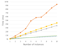
Figure 4: Our model keeps steady memory and time complexity when the number of instance increases. InstMatt’s complexity increases linearly with the number of instances.

Quantitative results. We evaluated our model against previous baselines after retraining them on our I-HIM50K dataset. Besides original works, we modified SparseMat’s first layer to accept a single mask input. Additionally, we expanded MGM to handle up to 10 instances, denoted as MGM^⋆. We also include the public weights of InstMatt [49] and MGM-in-the-wild [39]. The performance with different masks M-HIM2K are reported in Table 5. The public InstMatt showed the best performance, but this comparison may not be entirely fair as it was trained on private external data. Our model demonstrated comparable results on composite and natural sets, achieving the lowest error in most metrics. MGM^⋆ also performed well, suggesting that processing multiple masks simultaneously can facilitate instance interaction, although this approach slightly impacted the Grad metric, which reflects the output’s detail.

We also measure the memory and speed of models on M-HIM2K natural set in Fig. 4. While InstMatt, MGM, and SparseMat have the inference time increasing linearly to the number of instances, MGM^⋆ and ours keep steady performance in both memory and speed.

Table 6: Superiority of Temporal Consistency in Feature and Prediction Levels. Our MaGGIe, integrating temporal consistency at both feature and matte levels, outperforms non-temporal methods and those with only feature level.

Conv-GRU		Fusion		Easy		Medium		Hard
Single	Bi	$\mathbf{\hat{A}}^{f}$	$\mathbf{\hat{A}}^{b}$	MAD	dtSSD	MAD	dtSSD	MAD	dtSSD
				10.26	16.57	13.88	23.67	21.62	30.50
✓				10.15	16.42	13.84	23.66	21.26	29.95
	✓			10.14	16.41	13.83	23.66	21.25	29.92
	✓	✓		11.32	16.51	15.33	24.08	24.97	30.66
	✓	✓	✓	10.12	16.40	13.85	23.63	21.23	29.90

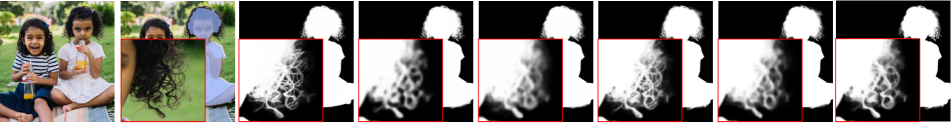
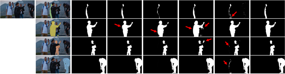
Image	Input mask	Groundtruth	InstMatt	InstMatt	MGM	MGM⋆	Ours

Figure 5: Enhanced Detail and Instance Separation by MaGGIe. Our model excels in rendering detailed outputs and effectively separating instances, as highlighted by red squares (detail focus) and red arrows (errors in other methods).

Table 7: Comparative Analysis of Video Matting Methods on V-HIM60. This table categorizes methods into two groups: those utilizing first-frame trimaps (upper group) and mask-guided approaches (lower group). Gray rows denotes models with public weights not retrained on I-HIM50K and V-HIM50K. MGM^⋆-TCVOM represents MGM with stacked guidance masks and the TCVOM temporal module. Bold and underline highlight the top and second-best performing models in each metric, respectively.

Method	Easy					Medium					Hard
	MAD	Grad	Conn	dtSSD	MESSDdt	MAD	Grad	Conn	dtSSD	MESSDdt	MAD	Grad	Conn	dtSSD	MESSDdt
First-frame trimap
OTVM [45]	204.59	15.25	76.36	46.58	397.59	247.97	21.02	97.74	66.09	587.47	412.41	29.97	146.11	90.15	764.36
OTVM [45]	36.56	6.62	14.01	24.86	69.26	48.59	10.19	17.03	36.06	80.38	140.96	17.60	47.84	59.66	298.46
FTP-VM [17]	12.69	6.03	4.27	19.83	18.77	40.46	12.18	15.13	32.96	125.73	46.77	14.40	15.82	45.04	76.48
FTP-VM [17]	13.69	6.69	4.78	20.51	22.54	26.86	12.39	9.95	32.64	126.14	48.11	14.87	16.12	45.29	78.66
Frame-by-frame binary mask
MGM-TCVOM [45]	11.36	4.57	3.83	17.02	19.69	14.76	7.17	5.41	23.39	39.22	22.16	7.91	7.27	31.00	47.82
MGM⋆-TCVOM [45]	10.97	4.19	3.70	16.86	15.63	13.76	6.47	5.02	23.99	42.71	22.59	7.86	7.32	32.75	37.83
InstMatt [49]	13.77	4.95	3.98	17.86	18.22	19.34	7.21	6.02	24.98	54.27	27.24	7.88	8.02	31.89	47.19
SparseMat [50]	12.02	4.49	4.11	19.86	24.75	18.20	8.03	6.87	30.19	85.79	24.83	8.47	8.19	36.92	55.98
MaGGIe (ours)	10.12	4.08	3.43	16.40	16.41	13.85	6.31	5.11	23.63	38.12	21.23	7.08	6.89	29.90	42.98

Qualitative results. MaGGIe’s ability to capture fine details and effectively separate instances is showcased in Fig. 5. At the exact resolution, our model not only achieves highly detailed outcomes comparable to running MGM separately for each instance but also surpasses both the public and retrained versions of InstMatt. A key strength of our approach is its proficiency in distinguishing between different instances. This is particularly evident when compared to MGM, where we observed overlapping instances, and MGM^⋆, which has noise issues caused by processing multiple masks simultaneously. Our model’s refined instance separation capabilities highlight its effectiveness in handling complex matting scenarios.

5.2 Training on video data

Temporal consistency metrics. Following previous works [57, 48, 45], we extended our evaluation metrics to include dtSSD and MESSDdt to assess the temporal consistency of instance matting across frames.

Ablation studies. Our tests, detailed in Table 6, show that each temporal module significantly impacts performance. Omitting these modules increased errors in all subsets. Single-direction Conv-GRU use improved outcomes, with further gains from adding backward pass fusion. Forward fusion alone was less effective, possibly due to error propagation. The optimal setup involved combining backward propagation to reduce errors, yielding the best results.

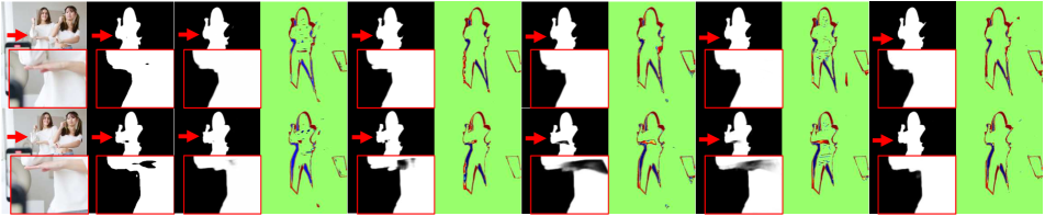
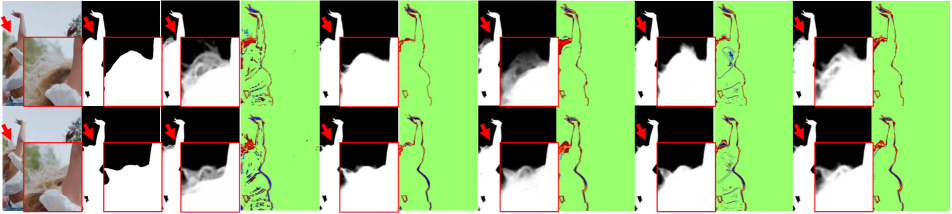
Frame	Input mask	$\hat{\mathbf{A}}$	$\log\mathopen{}\left|\Delta_{\hat{\mathbf{A}}}\mathclose{}\right|$	$\hat{\mathbf{A}}$	$\log\mathopen{}\left|\Delta_{\hat{\mathbf{A}}}\mathclose{}\right|$	$\hat{\mathbf{A}}$	$\log\mathopen{}\left|\Delta_{\hat{\mathbf{A}}}\mathclose{}\right|$	$\hat{\mathbf{A}}$	$\log\mathopen{}\left|\Delta_{\hat{\mathbf{A}}}\mathclose{}\right|$	$\hat{\mathbf{A}}$	$\log\mathopen{}\left|\Delta_{\hat{\mathbf{A}}}\mathclose{}\right|$
		$\underbrace{\hskip 73.97733pt}_{\begin{subarray}{c}\vspace{-5.0mm}\end{subarray}\hbox{\pagecolor{white}~{}~{}InstMatt~{}~{}}}$		$\underbrace{\hskip 73.97733pt}_{\begin{subarray}{c}\vspace{-5.0mm}\end{subarray}\hbox{\pagecolor{white}~{}~{}SparseMat~{}~{}}}$		$\underbrace{\hskip 73.97733pt}_{\begin{subarray}{c}\vspace{-5.0mm}\end{subarray}\hbox{\pagecolor{white}~{}~{}MGM-TCVOM~{}~{}}}$		$\underbrace{\hskip 73.97733pt}_{\begin{subarray}{c}\vspace{-5.0mm}\end{subarray}\hbox{\pagecolor{white}~{}~{}MGM${}^{\star}$-TCVOM~{}~{}}}$		$\underbrace{\hskip 73.97733pt}_{\begin{subarray}{c}\vspace{-5.0mm}\end{subarray}\hbox{\pagecolor{white}~{}~{}MaGGIe (ours)~{}~{}}}$

Figure 6: Detail and Consistency in Frame-to-Frame Predictions. This figure demonstrates the precision and temporal consistency of our model’s alpha matte predictions, highlighting robustness against noise from input masks. The color-coded map (min-max range) to illustrate differences between consecutive frames is .

Performance evaluation. Our model was benchmarked against leading methods in trimap video matting, mask-guided matting, and instance matting. For trimap video matting, we chose OTVM [45] and FTP-VM [17], fine-tuning them on our V-HIM2K5 dataset. In masked guided video matting, we compared our model with InstMatt [49], SparseMat [50], and MGM [56] which is combined with the TCVOM [57] module for temporal consistency. InstMatt, after being fine-tuned on I-HIM50K and subsequently on V-HIM2K5, processed each frame in the test set independently, without temporal awareness. SparseMat, featuring a temporal sparsity fusion module, was fine-tuned under the same conditions as our model. MGM and its variant, integrated with the TCVOM module, emerged as strong competitors in our experiments, demonstrating their robustness in maintaining temporal consistency across frames.

The comprehensive results of our model across three test sets, using masks from XMem, are detailed in Table 7. All trimap propagation methods are underperform the mask-guided solutions. When benchmarked against other masked guided matting methods, our approach consistently reduces error across most metrics. Notably, it excels in temporal consistency, evidenced by its top performance in dtSSD for both easy and hard test sets, and in MESSDdt for the medium set. Additionally, our model shows superior performance in capturing fine details, as indicated by its leading scores in the Grad metric across all test sets. These results underscore our model’s effectiveness in video instance matting, particularly in challenging scenarios requiring high temporal consistency and detail preservation.

Temporal consistency and detail preservation. Our model’s effectiveness in video instance matting is evident in Fig. 6 with natural videos. Key highlights include:

• Handling of Random Noises: Our method effectively handles random noise in mask inputs, outperforming others that struggle with inconsistent input mask quality.

• Foreground/Background Region Consistency: We maintain consistent, accurate foreground predictions across frames, surpassing InstMatt and MGM^⋆-TCVOM.

• Detail Preservation: Our model retains intricate details, matching InstMatt’s quality and outperforming MGM variants in video inputs.

These aspects underscore MaGGIe’s robustness and effectiveness in video instance matting, particularly in maintaining temporal consistency and preserving fine details across frames.

6 Discussion

Limitation and Future work. Our MaGGIe demonstrates effective performance in human video instance matting with binary mask guidance, yet it also presents opportunities for further research and development. One notable limitation is the reliance on one-hot vector representation for each location in the guidance mask, necessitating that each pixel is distinctly associated with a single instance. This requirement can pose challenges, particularly when integrating instance masks from varied sources, potentially leading to misalignments in certain regions. Additionally, the use of composite training datasets may constrain the model’s ability to generalize effectively to natural, real-world scenarios. While the creation of a comprehensive natural dataset remains a valuable goal, we propose an interim solution: the utilization of segmentation datasets combined with self-supervised or weakly-supervised learning techniques. This approach could enhance the model’s adaptability and performance in more diverse and realistic settings, paving the way for future advancements in the field.

Conclusion. Our study contributes to the evolving field of instance matting, with a focus that extends beyond human subjects. By integrating advanced techniques like transformer attention and sparse convolution, MaGGIe shows promising improvements over previous methods in detailed accuracy, temporal consistency, and computational efficiency for both image and video inputs. Additionally, our approach in synthesizing training data and developing a comprehensive benchmarking schema offers a new way to evaluate the robustness and effectiveness of models in instance matting tasks. This work represents a step forward in video instance matting and provides a foundation for future research in this area.

Acknownledgement. We sincerely appreciate Markus Woodson for the invaluable initial discussions. Additionally, I am deeply thankful to my wife, Quynh Phung, for her meticulous proofreading and feedback.

Supplementary Material

7 Architecture details

This section delves into the architectural nuances of our framework, providing a more detailed exposition of components briefly mentioned in the main paper. These insights are crucial for a comprehensive understanding of the underlying mechanisms of our approach.

7.1 Mask guidance identity embedding

We embed mask guidance into a learnable space before inputting it into our network. This approach, inspired by the ID assignment in AOT [55], generates a guidance embedding $\mathbf{E}\in\mathbb{R}^{T\times C_{e}\times H\times W}$ by mapping embedding vectors $\mathbf{D}\in\mathbb{R}^{N\times C_{e}}$ to pixels based on the guidance mask $\mathbf{M}$:

$$\mathbf{E}(x,y)=\mathbf{M}(x,y)\mathbf{D}.$$ (4)

Here, $\mathbf{E}(x,y)\in\mathbb{R}^{T\times C_{e}}$ and $\mathbf{M}(x,y)\in\{0,1\}^{T\times N}$ represent the values at row $y$ and column $x$ in $\mathbf{E}$ and $\mathbf{M}$, respectively. In our experiment, we set $N=10$, but it can be any larger number without affecting the architecture significantly.

7.2 Feature extractor

In our experiments, we employ ResNet-29 [13] as the feature extractor, consistent with other baselines [56, 49]. We have $C_{8}=128,C_{4}=64,C_{1}=C_{2}=32$.

7.3 Dense-image to sparse-instance features

We express the Eq. (2) as the visualization in Fig. 7. It involves extracting feature vectors $\mathbf{\bar{F}}(x,y,t)$ and instance token vectors $\mathbf{T}_{i}$ for each uncertainty index $(x,y,t,i)\in\mathbf{U}$. These vectors undergo channel-wise multiplication, emphasizing channels relevant to each instance. A subsequent MLP layer then converts this product into sparse, instance-specific features.

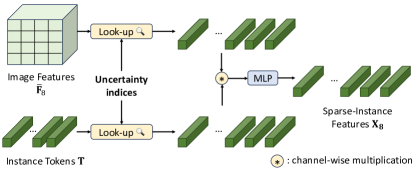
Figure 7: Converting Dense-Image to Sparse-Instance Features. We transform the dense image features into sparse, instance-specific features with the help of instance tokens.

7.4 Detail aggregation

This process, akin to a U-net decoder, aggregates features from different scales, as detailed in Fig. 8. It involves upscaling sparse features and merging them with corresponding higher-scale features. However, this requires pre-computed downscale indices from dummy sparse convolutions on the full input image.

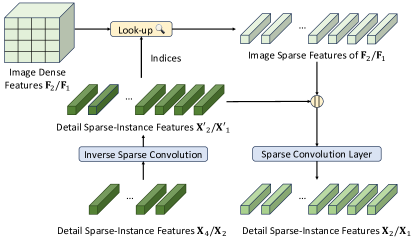
Figure 8: Detail Aggregation Module merges sparse features across scales. This module equalizes spatial scales of sparse features using inverse sparse convolution, facilitating their combination.

7.5 Sparse matte head

Our matte head design, inspired by MGM [56], comprises two sparse convolutions with intermediate normalization and activation (Leaky ReLU) layers. The final output undergoes sigmoid activation for the final prediction. Non-refined locations in the dense prediction are assigned a value of zero.

7.6 Sparse progressive refinement

The PRM module progressively refines $\mathbf{A}_{8}\rightarrow\mathbf{A}_{4}\rightarrow\mathbf{A}_{1}$ to have $\mathbf{A}$. We assume that all predictions are rescaled to the largest size and perform refinement between intermediate predictions and uncertainty indices $\mathbf{U}$:

$$\mathbf{A} =\mathbf{A}_{8}$$ (5)

$$\mathbf{R}_{4}(j) =\begin{cases}1\text{, if }j\in\mathcal{D}(\mathbf{A})\text{ and }j\in\mathbf{U}\\ 0\text{, otherwise }\end{cases}$$ (6)

$$\mathbf{A} =\mathbf{A}\times(1-\mathbf{R}_{4})+\mathbf{R}_{4}\times\mathbf{A}_{4}$$ (7)

$$\mathbf{R}_{1}(j) =\begin{cases}1\text{, if }j\in\mathcal{D}(\mathbf{A})\text{ and }j\in\mathbf{U}\\ 0\text{, otherwise }\end{cases}$$ (8)

$$\mathbf{A} =\mathbf{A}\times(1-\mathbf{R}_{1})+\mathbf{R}_{1}\times\mathbf{A}_{4}$$ (9)

where $j=(x,y,t,i)$ is an index in the output; $\mathbf{R}_{1},\mathbf{R}_{4}$ in shape $T\times N\times H\times W$; and $\mathcal{D}(\mathbf{A})=\text{dilation}(0<\mathbf{A}<1)$ is the indices of all dilated uncertainty values on $\mathbf{A}$. The dilation kernel is set to 30, 15 for $\mathbf{R}_{4},\mathbf{R}_{1}$ respectively.

7.7 Attention loss and loss weight

With $\mathbf{A}^{gt}$ as the ground-truth alpha matte and its $\frac{1}{8}$ downscaled version $\mathbf{A}^{gt}_{8}$, we define a binarized $\mathbf{\tilde{A}}^{gt}_{8}=\mathbf{A}^{gt}_{8}>0$. The attention loss $\mathcal{L}_{\text{att}}$ is:

$$\mathcal{L}_{\text{att}}=\sum_{i}^{N}\left\|\mathbf{1}-\text{Aff}(i)^{\top}\mathbf{\tilde{A}}^{gt}_{8}(i)\right\|_{1}$$ (10)

aiming to maximize each instance token $\mathbf{T}_{i}$’s attention score to its corresponding groundtruth region $\mathbf{\tilde{A}}^{gt}_{8}(i)$.

The weight $\mathbf{W}_{8}$ at each location is:

$$\mathbf{W}_{8}(j)=\begin{cases}\gamma,\text{ if }0<\mathbf{A}^{gt}_{8}(j)<1\text{ and }0<\mathbf{A}_{8}(j)<1\\ 1.0,\text{ otherwise }\end{cases}$$ (11)

with $\gamma=2.0$ in our experiments, focusing on under-refined ground-truth and over-refined predicted areas.

7.8 Temporal sparsity prediction

A key aspect of our approach is the prediction of temporal sparsity to maintain consistency between frames. This module contrasts the feature maps of consecutive frames to predict their absolute differences. Comprising three convolution layers with batch normalization and ReLU activation, this module processes the concatenated feature maps from two adjacent frames and predicts the binary differences between them.

Unlike SparseMat [50], which relies on manual threshold selection for frame differences, our method offers a more robust and domain-independent approach to determining frame sparsity. This is particularly effective in handling variations in movement, resolution, and domain between frames, as demonstrated in Fig. 9

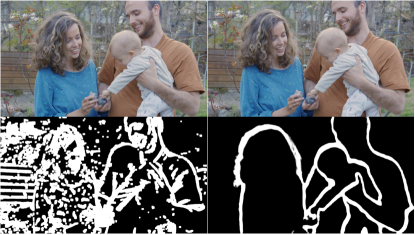
SparseMat [50]

Ours

Figure 9: Temporal Sparsity Between Two Consecutive Frames. The top row displays a pair of successive frames. Below, the second row illustrates the predicted differences by two distinct frameworks, with areas of discrepancy emphasized in white. In contrast to SparseMat’s output, which appears cluttered and noisy, our module generates a more refined sparsity map. This map effectively accentuates the foreground regions that undergo notable changes between the frames, providing a clearer and more focused representation of temporal sparsity. (Best viewed in color).

7.9 Forward and backward matte fusion

The forward-backward fusion for the $i$-th instance at frame $t$ is respectively:

$$\begin{split}\mathbf{A}^{f}(t,i)&=\Delta(t)\times\mathbf{A}(t,i)\\ &+(1-\Delta(t))\times\mathbf{A}^{f}(t-1,i)\\ \end{split}$$ (12)

$$\begin{split}\ \mathbf{A}^{b}(t,i)&=\Delta(t+1)\times\mathbf{A}(t,i)\\ &+(1-\Delta(t+1))\times\mathbf{A}^{b}(t+1,i)\\ \end{split}$$ (13)

Each entry $j=(x,y,t,i)$ on final output $\mathbf{A}^{\text{temp}}$ is:

$$\mathbf{A}^{\text{temp}}(j)=\begin{cases}\mathbf{A}(j),\text{ if }\mathbf{A}^{f}(j)\neq\mathbf{A}^{b}(j)\\ \mathbf{A}^{f}(j),\text{ otherwise}\end{cases}$$ (14)

This fusion enhances temporal consistency and minimizes error propagation.

8 Image matting

This section expands on the image matting process, providing additional insights into dataset generation and comprehensive comparisons with existing methods. We delve into the creation of I-HIM50K and M-HIM2K datasets, offer detailed quantitative analyses, and present further qualitative results to underscore the effectiveness of our approach.

8.1 Dataset generation and preparation

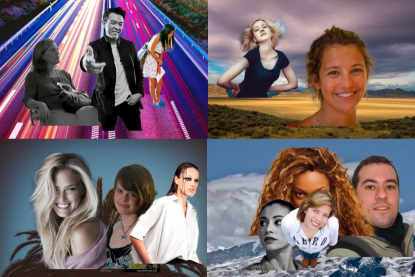
Figure 10: Examples of I-HIM50K dataset. (Best viewed in color).

The I-HIM50K dataset was synthesized from the HHM50K [50] dataset, which is known for its extensive collection of human image mattes. We employed a MaskRCNN [14] Resnet-50 FPN 3x model, trained on the COCO dataset, to filter out single-person images, resulting in a subset of 35,053 images. Following the InstMatt [49] methodology, these images were composited against diverse backgrounds from the BG20K [29] dataset, creating multi-instance scenarios with 2-5 subjects per image. The subjects were resized and positioned to maintain a realistic scale and avoid excessive overlap, as indicated by instance IoUs not exceeding 30%. This process yielded 49,737 images, averaging 2.28 instances per image. During training, guidance masks were generated by binarizing the alpha mattes and applying random dropout, dilation, and erosion operations. Sample images from I-HIM50K are displayed in Fig. 10.

Table 8: Ten models with vary mask quality are used in M-HIM2K. The MaskRCNN models are from detectron2 trained on COCO with different settings.

Model	COCO mask AP (%)
r50_c4_3x	34.4
r50_dc5_3x	35.9
r101_c4_3x	36.7
r50_fpn_3x	37.2
r101_fpn_3x	38.6
x101_fpn_3x	39.5
r50_fpn_400e	42.5
regnety_400e	43.3
regnetx_400e	43.5
r101_fpn_400e	43.7

The M-HIM2K dataset was designed to test model robustness against varying mask qualities. It comprises ten masks per instance, generated using various MaskRCNN models. More information about models used for this generation process is shown in Table 8. The masks were matched to instances based on the highest IoU with the ground truth alpha mattes, ensuring a minimum IoU threshold of 70%. Masks that did not meet this threshold were artificially generated from ground truth. This process resulted in a comprehensive set of 134,240 masks, with 117,660 for composite and 16,600 for natural images, providing a robust benchmark for evaluating masked guided instance matting. The full dataset I-HIM50K and M-HIM2K will be released after the acceptance of this work.

Table 9: Full details of different input mask setting on HIM2K+M-HIM2K. (Extension of Table 3). Bold denotes the lowest average error.

Mask input	Composition							Natural
	MAD	MADf	MADu	MSE	SAD	Grad	Conn	MAD	MADf	MADu	MSE	SAD	Grad	Conn
Stacked	27.01	68.83	381.27	18.82	16.35	16.80	15.72	39.29	61.39	213.27	25.10	25.52	16.44	23.26	mean
	0.83	5.93	7.06	0.76	0.50	0.31	0.51	4.21	13.37	14.10	4.01	2.00	0.70	2.02	std
Embeded($C_{e}=1$)	19.18	68.04	330.06	12.40	11.64	13.00	11.16	33.60	60.35	188.44	20.63	21.40	13.44	19.18	mean
	0.87	8.07	6.96	0.80	0.52	0.27	0.52	4.07	12.60	12.28	3.86	1.81	0.57	1.83	std
Embeded($C_{e}=2$)	21.74	84.64	355.95	14.46	13.23	14.39	12.69	35.16	59.55	193.95	21.93	22.59	14.51	20.40	mean
	0.92	7.33	7.68	0.85	0.55	0.27	0.55	4.23	13.79	13.45	4.03	2.31	0.61	2.32	std
Embeded($C_{e}=3$)	17.75	53.23	315.43	11.19	10.79	12.52	10.32	33.06	56.69	189.59	20.22	19.43	13.11	17.30	mean
	0.66	5.04	6.31	0.60	0.39	0.24	0.39	3.74	11.90	12.49	3.58	1.92	0.51	1.95	std
Embeded($C_{e}=5$)	24.79	73.22	384.14	17.07	15.09	16.19	14.58	34.25	65.57	216.56	20.39	21.89	15.66	19.70	mean
	0.88	4.99	7.24	0.79	0.52	0.30	0.52	4.16	13.59	13.09	3.96	2.31	0.58	2.32	std

Table 10: Full details of different training objective components on HIM2K+M-HIM2K. (Extension of Table 4). Bold denotes the lowest average error.

$\mathcal{L}_{att}$	$\mathbf{W}_{8}$	Composition							Natural
		MAD	MADf	MADu	MSE	SAD	Grad	Conn	MAD	MADf	MADu	MSE	SAD	Grad	Conn
		31.77	52.70	294.22	24.13	18.92	16.58	18.27	46.68	51.23	176.60	33.61	32.89	15.68	30.64	mean
		0.90	4.92	5.24	0.85	0.54	0.26	0.54	3.64	10.27	9.58	3.47	1.85	0.50	1.85	std
	✓	25.41	104.24	342.19	18.36	15.29	14.53	14.75	46.30	87.18	210.72	32.93	31.40	15.84	29.26	mean
		0.72	6.15	5.53	0.67	0.43	0.23	0.43	3.71	11.68	10.62	3.55	1.85	0.50	1.86	std
✓		17.56	53.51	302.07	11.24	10.65	12.34	10.22	32.95	51.11	183.13	20.41	19.23	13.29	17.06	mean
		0.75	6.32	6.32	0.70	0.45	0.27	0.45	3.34	10.25	10.99	3.19	2.04	0.60	2.06	std
✓	✓	17.55	47.81	301.96	11.23	10.68	12.34	10.19	32.03	53.15	183.42	19.42	19.60	13.16	17.43	mean
		0.68	5.21	5.73	0.63	0.41	0.25	0.41	3.48	10.77	11.18	3.32	1.92	0.55	1.94	std

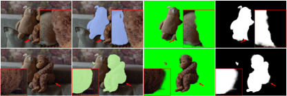
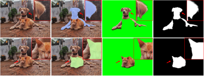
Image

Mask

Foreground

Alpha matte

Figure 11: Our framework can generalize to any object. Without humans appearing in the image, our framework still performs the matting task very well to the mask-guided objects. (Best viewed in color and digital zoom).

8.2 Training details

We initialized our feature extractor with ImageNet [43] weights, following previous methods [56, 49]. Our models were retrained on the I-HIM50K dataset with a crop size 512. All baselines underwent 100 training epochs, using the HIM2K composition set for validation. The training was conducted on 4 A100 GPUs with a batch size 96. We employed AdamW for optimization, with a learning rate of $1.5\times 10^{-4}$ and a cosine decay schedule post 1,500 warm-up iterations. The training also incorporated curriculum learning as MGM and standard augmentation as other baselines. During training, mask orders were shuffled, and some masks were randomly omitted. In testing, images were resized to have a short side of 576 pixels.

8.3 Quantitative details

We extend the ablation study from the main paper, providing detailed statistics in Table 9 and Table 10. These tables offer insights into the average and standard deviation of performance metrics across HIM2K [49] and M-HIM2K datasets. Our model not only achieves competitive average results but also maintains low variability in performance across different error metrics. Additionally, we include the Sum Absolute Difference (SAD) metric, aligning with previous image matting benchmarks.

Comprehensive quantitative results comparing our model with baseline methods on HIM2K and M-HIM2K are presented in Table LABEL:tab:details. This analysis highlights the impact of mask quality on matting output, with our model demonstrating consistent performance even with varying mask inputs.

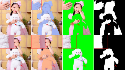
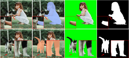
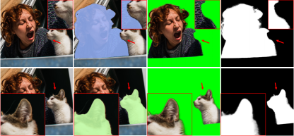
Image

Mask

Foreground

Alpha matte

Figure 12: Our solution is not limited to human instances. When testing with other objects, our solution is able to produce fairly accurate alpha matte without training on them. (Best viewed in color and digital zoom).

Table 11: Compare between previous dense progressive refinement (PR) - MGM and our proposed guided sparse progressive refinement. Numbers are mean on HIM2K+M-HIM2K and small numbers indicate the std.

PR	MAD	MSE	Grad	Conn	MADf	MADu
Comp Set
MGM	14.70 (0.4)	8.87 (0.3)	10.39 (0.2)	8.44 (0.2)	32.02 (1.5)	252.34 (4.2)
Ours	12.93 (0.3)	7.26 (0.3)	8.91 (0.1)	7.37 (0.2)	19.54 (1.0)	235.95 (3.4)
Natural Set
MGM	27.66 (4.1)	16.94 (3.9)	10.49 (0.7)	13.95 (1.5)	52.72 (12.1)	150.71 (13.3)
Ours	27.17 (3.3)	16.09 (3.2)	9.94 (0.6)	13.42 (1.4)	49.52 (8.0)	146.71 (11.6)

We also perform another experiment when the MGM-style refinement replaces our proposed sparse guided progressive refinement. The Table 11 shows the results where our proposed method outperforms the previous approach in all metrics.

8.4 More qualitative results on natural images

Fig. 13 showcases our model’s performance in challenging scenarios, particularly in accurately rendering hair regions. Our framework consistently outperforms MGM^⋆ in detail preservation, especially in complex instance interactions. In comparison with InstMatt, our model exhibits superior instance separation and detail accuracy in ambiguous regions.

Fig. 14 and Fig. 15 illustrate the performance of our model and previous works in extreme cases involving multiple instances. While MGM^⋆ struggles with noise and accuracy in dense instance scenarios, our model maintains high precision. InstMatt, without additional training data, shows limitations in these complex settings.

The robustness of our mask-guided approach is further demonstrated in Fig. 16. Here, we highlight the challenges faced by MGM variants and SparseMat in predicting missing parts in mask inputs, which our model addresses. However, it is important to note that our model is not designed as a human instance segmentation network. As shown in Fig. 17, our framework adheres to the input guidance, ensuring precise alpha matte prediction even with multiple instances in the same mask.

Lastly, Fig. 12 and Fig. 11 emphasize our model’s generalization capabilities. The model accurately extracts both human subjects and other objects from backgrounds, showcasing its versatility across various scenarios and object types.

All examples are Internet images without groundtruth and the mask from r101_fpn_400e are used as the guidance.

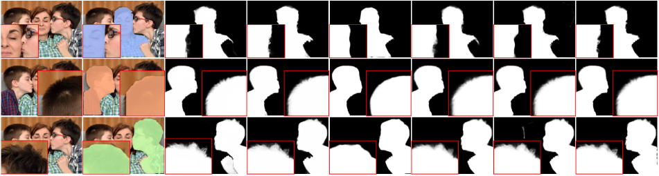
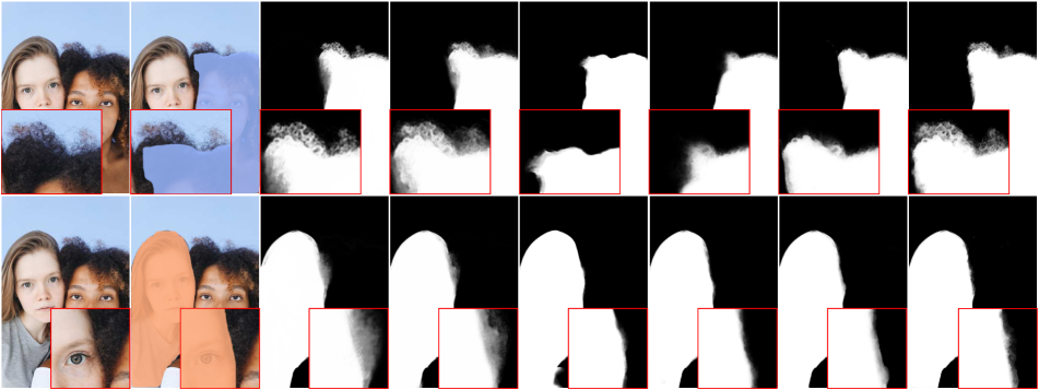
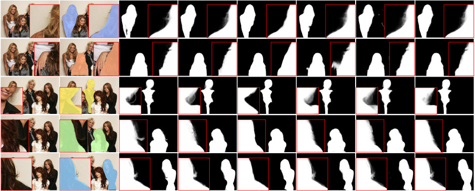
Image	Mask	InstMatt [49] (public)	InstMatt [49]	SparseMat
[50]	MGM [56]	MGM⋆	Ours

Figure 13: Our model produces highly detailed alpha matte on natural images. Our results show that it is accurate and comparable with previous instance-agnostic and instance-awareness methods without expensive computational costs. Red squares zoom in the detail regions for each instance. (Best viewed in color and digital zoom).

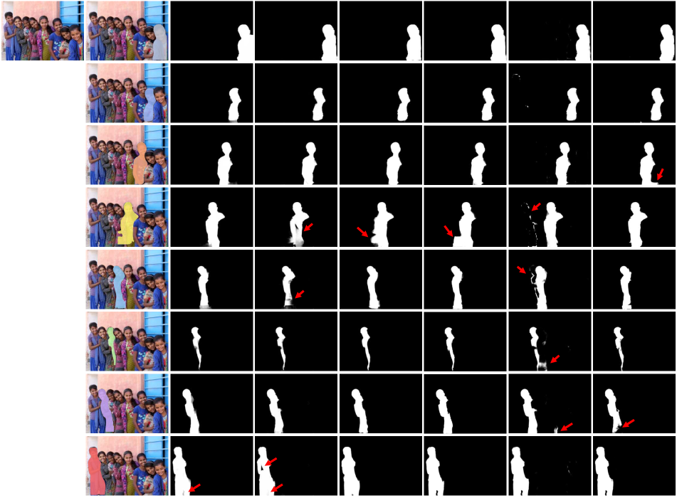
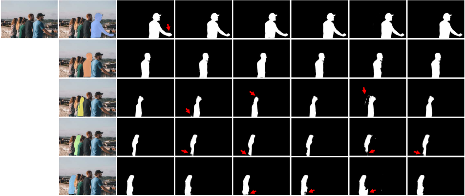
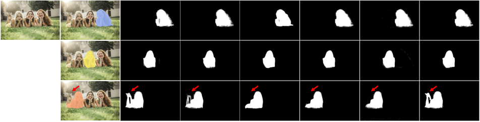
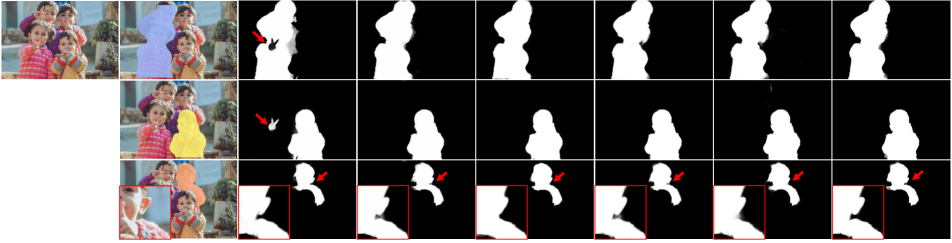
Image	Mask	InstMatt [49] (public)	InstMatt [49]	SparseMat
[50]	MGM [56]	MGM⋆	Ours

Figure 14: Our frameworks precisely separate instances in an extreme case with many instances. While MGM often causes the overlapping between instances and MGM^⋆ contains noises, ours produces on-par results with InstMatt trained on the external dataset. Red arrow indicates the errors. (Best viewed in color and digital zoom).

Image	Mask	InstMatt [49] (public)	InstMatt [49]	SparseMat
[50]	MGM [56]	MGM⋆	Ours

Figure 15: Our frameworks precisely separate instances in a single pass. The proposed solution shows comparable results with InstMatt and MGM without running the prediction/refinement five times. Red arrow indicates the errors. (Best viewed in color and digital zoom).

Image	Mask	InstMatt [49] (public)	InstMatt [49]	SparseMat
[50]	MGM [56]	MGM⋆	Ours

Figure 16: Unlike MGM and SparseMat, our model is robust to the input guidance mask. With the attention head, our model produces more stable results to mask inputs without complex refinement between instances like InstMatt. Red arrow indicates the errors. (Best viewed in color and digital zoom).

Image	Mask	InstMatt [49] (public)	InstMatt [49]	SparseMat
[50]	MGM [56]	MGM⋆	Ours

Figure 17: Our solution works correctly with multi-instance mask guidances. When multiple instances exist in one guidance mask, we still produce the correct union alpha matte for those instances. Red arrow indicates the errors or the zoom-in region in red box. (Best viewed in color and digital zoom).

[ theme=cvpr, caption=Details of quantitative results on HIM2K+M-HIM2K (Extension of Table 5). Gray indicates the public weight without retraining. , label=tab:details ] width=rows = font=, row4-15,41-52=gainsboro, colspec=@c—ccccccc—ccccccc—l@ Model Composition set Natural set Mask from MAD MAD_f MAD_u MSE SAD Grad Conn MAD MAD_f MAD_u MSE SAD Grad Conn Instance-agnostic MGM [39] 25.79 69.67 331.73 17.00 15.65 13.64 14.91 48.05 103.81 233.85 32.66 27.44 14.72 25.07 r50_c4_3x 24.75 70.92 316.59 16.21 15.01 13.17 14.23 34.67 66.28 183.48 21.03 22.82 12.79 20.30 r50_dc5_3x 23.60 66.79 321.23 15.03 14.38 13.19 13.62 35.51 70.94 198.99 20.96 22.62 13.73 20.17 r101_c4_3x 24.55 67.27 316.29 15.97 14.91 13.14 14.12 33.66 67.41 184.99 19.93 21.99 13.06 19.43 r50_fpn_3x 23.42 66.37 310.99 14.94 14.21 12.84 13.42 35.14 72.30 183.87 21.02 21.87 12.82 19.34 r101_fpn_3x 22.71 63.35 305.67 14.36 13.81 12.64 13.03 31.06 61.76 175.33 17.60 20.98 12.61 18.44 x101_fpn_3x 22.03 61.91 300.29 13.85 13.36 12.30 12.59 29.16 57.59 165.22 15.93 20.10 11.76 17.56 r50_fpn_400e 21.37 57.28 296.73 13.18 12.98 12.16 12.21 26.40 51.24 158.95 13.42 17.73 11.45 15.10 regnety_400e 21.78 60.31 297.14 13.62 13.22 12.25 12.46 27.09 49.26 160.05 13.82 17.48 11.20 14.87 regnetx_400e 21.52 60.07 297.14 13.44 13.14 12.20 12.38 24.41 51.46 152.90 11.62 17.43 11.09 14.84 r101_fpn_400e 23.15 64.39 309.38 14.76 14.07 12.75 13.30 32.52 65.20 179.76 18.80 21.05 12.52 18.51 mean 1.52 4.49 12.01 1.30 0.92 0.52 0.92 6.74 15.94 23.87 5.99 3.09 1.17 3.16 std MGM [56] 15.94 32.55 266.64 9.62 9.68 10.11 9.18 37.55 86.64 191.09 24.03 21.15 11.34 18.94 r50_c4_3x 16.05 36.36 264.96 9.81 9.75 10.10 9.26 32.58 68.52 172.83 19.58 20.17 10.92 17.80 r50_dc5_3x 15.40 30.89 264.28 9.17 9.37 10.01 8.90 31.24 69.59 175.67 18.15 18.57 10.83 16.26 r101_c4_3x 15.93 34.54 265.44 9.68 9.67 10.10 9.20 32.83 75.06 173.63 19.72 19.13 10.85 16.81 r50_fpn_3x 15.74 34.23 263.35 9.50 9.55 10.02 9.07 30.77 69.10 171.92 17.78 18.22 10.67 15.95 r101_fpn_3x 15.23 36.18 260.80 9.03 9.27 9.92 8.76 30.09 63.23 167.58 17.34 18.51 10.69 16.09 x101_fpn_3x 14.96 34.13 259.17 8.81 9.08 9.83 8.61 28.28 50.35 158.02 15.71 17.71 10.24 15.25 r50_fpn_400e 14.53 31.71 256.33 8.41 8.83 9.73 8.35 26.95 49.55 155.63 14.43 15.69 9.98 13.34 regnety_400e 14.82 33.06 257.09 8.69 9.01 9.80 8.53 26.61 47.81 154.05 14.22 15.45 9.87 13.16 regnetx_400e 14.65 31.71 256.29 8.53 8.94 9.74 8.46 25.42 51.73 153.11 13.03 15.73 9.90 13.44 r101_fpn_400e 15.32 33.54 261.43 9.13 9.31 9.94 8.83 30.23 63.16 167.35 17.40 18.03 10.53 15.70 mean 0.57 1.88 4.00 0.51 0.34 0.15 0.34 3.62 12.97 12.14 3.26 1.93 0.50 1.94 std SparseMat [50] 23.14 47.59 378.89 16.37 13.97 15.56 13.54 46.28 101.48 255.98 31.99 26.81 17.97 24.82 r50_c4_3x 21.94 49.48 358.08 15.36 13.24 14.90 12.80 36.93 67.62 213.46 23.76 22.11 16.05 20.01 r50_dc5_3x 21.78 43.36 368.59 15.15 13.16 15.21 12.72 38.32 77.98 234.69 24.51 22.83 17.19 20.78 r101_c4_3x 21.94 47.00 361.30 15.33 13.24 14.99 12.80 37.16 74.18 218.62 23.95 21.95 16.39 19.86 r50_fpn_3x 21.43 46.51 356.43 14.88 12.93 14.81 12.48 35.95 72.78 218.46 22.62 20.67 16.11 18.58 r101_fpn_3x 20.63 47.73 349.81 14.12 12.48 14.58 12.02 34.32 64.51 209.64 21.10 20.44 16.03 18.33 x101_fpn_3x 20.29 44.20 342.14 13.93 12.22 14.21 11.76 31.44 57.51 197.53 18.58 19.49 14.96 17.35 r50_fpn_400e 19.65 41.20 340.38 13.29 11.85 14.08 11.38 30.21 48.53 194.90 17.32 17.47 14.82 15.31 regnety_400e 19.90 41.40 336.40 13.56 12.02 14.03 11.56 29.85 52.17 191.09 16.99 17.19 14.52 15.03 regnetx_400e 19.81 43.43 337.43 13.50 12.01 14.05 11.55 29.83 61.40 191.89 17.07 17.13 14.48 14.96 r101_fpn_400e 21.05 45.19 352.95 14.55 12.71 14.64 12.26 35.03 67.82 212.63 21.79 20.61 15.85 18.50 mean 1.17 2.85 14.24 1.02 0.70 0.54 0.71 5.13 15.19 20.77 4.68 3.03 1.16 3.08 std Instance-awareness InstMatt [49] 12.98 23.71 257.74 5.76 7.94 9.47 7.27 31.15 60.03 174.10 15.91 18.12 10.64 15.73 r50_c4_3x 13.15 23.08 257.38 5.96 8.05 9.48 7.38 28.05 51.53 164.19 13.63 16.89 10.33 14.53 r50_dc5_3x 12.99 22.42 257.52 5.79 7.93 9.47 7.26 27.06 48.52 162.72 12.90 16.06 10.29 13.68 r101_c4_3x 13.13 20.60 256.70 5.90 8.03 9.47 7.36 28.31 49.87 164.16 13.97 16.86 10.37 14.49 r50_fpn_3x 13.04 23.98 257.51 5.85 7.96 9.45 7.28 28.92 59.32 168.72 14.37 16.98 10.40 14.64 r101_fpn_3x 12.77 22.16 255.33 5.63 7.83 9.40 7.16 27.02 46.39 162.89 12.82 16.49 10.27 14.08 x101_fpn_3x 12.61 21.31 254.27 5.55 7.71 9.36 7.05 25.33 44.84 157.03 11.23 15.54 9.97 13.18 r50_fpn_400e 12.58 23.53 253.85 5.57 7.69 9.35 7.03 24.34 41.62 154.89 10.65 15.22 10.00 12.85 regnety_400e 12.59 20.48 252.68 5.53 7.71 9.35 7.04 24.18 40.96 154.69 10.09 14.68 9.82 12.28 regnetx_400e 12.67 21.14 253.13 5.60 7.75 9.35 7.09 23.22 43.23 151.78 9.67 15.00 9.88 12.60 r101_fpn_400e 12.85 22.24 255.61 5.71 7.86 9.41 7.19 26.76 48.63 161.52 12.52 16.18 10.20 13.81 mean 0.23 1.31 2.00 0.16 0.14 0.06 0.13 2.48 6.76 6.94 2.05 1.08 0.26 1.08 std InstMatt [49] 18.23 57.23 298.66 10.51 11.06 11.33 10.45 37.91 86.84 202.20 22.28 21.31 12.22 19.11 r50_c4_3x 17.85 58.98 291.50 10.38 10.87 11.13 10.27 30.10 63.83 173.94 15.90 18.01 11.25 15.82 r50_dc5_3x 17.25 51.21 292.66 9.80 10.50 11.13 9.90 30.22 59.65 178.94 15.62 17.49 11.55 15.23 r101_c4_3x 17.69 55.80 292.90 10.22 10.80 11.19 10.19 30.27 60.16 175.66 16.44 17.38 11.33 15.13 r50_fpn_3x 17.18 55.67 288.95 9.85 10.45 11.02 9.84 28.80 60.88 170.89 14.55 16.88 11.12 14.69 r101_fpn_3x 16.65 53.37 284.66 9.41 10.16 10.85 9.56 27.77 55.06 168.20 14.14 16.91 11.04 14.70 x101_fpn_3x 16.29 52.00 281.15 9.21 9.88 10.69 9.29 25.51 52.89 156.40 12.15 15.90 10.47 13.70 r50_fpn_400e 15.99 50.92 279.15 8.97 9.71 10.65 9.12 24.82 45.83 156.46 11.83 15.14 10.43 12.94 regnety_400e 16.47 51.85 280.00 9.37 10.01 10.69 9.42 23.73 47.85 153.70 10.35 14.69 10.17 12.49 regnetx_400e 16.30 50.58 279.40 9.29 9.95 10.63 9.36 22.47 45.33 150.96 9.72 14.71 10.17 12.50 r101_fpn_400e 16.99 53.76 286.90 9.70 10.34 10.93 9.74 28.16 57.83 168.74 14.30 16.84 10.98 14.63 mean 0.76 2.96 6.95 0.53 0.47 0.26 0.46 4.45 12.15 15.45 3.65 1.97 0.66 1.97 std MGM^⋆ 14.87 46.70 256.01 8.32 8.99 10.31 8.32 37.36 65.40 181.68 23.97 20.50 11.66 17.45 r50_c4_3x 14.65 43.00 253.75 8.21 8.87 10.25 8.22 33.70 60.48 172.03 20.83 18.51 11.29 15.93 r50_dc5_3x 14.36 38.88 252.30 7.89 8.71 10.19 8.04 33.95 60.54 173.47 20.59 17.94 11.24 15.30 r101_c4_3x 14.68 44.85 254.50 8.21 8.88 10.24 8.22 33.29 54.82 170.89 20.21 18.28 11.27 15.55 r50_fpn_3x 14.70 44.68 254.29 8.24 8.89 10.21 8.25 32.07 68.47 171.41 18.80 17.44 11.07 14.84 r101_fpn_3x 14.27 43.56 251.19 7.83 8.68 10.13 8.00 30.96 50.90 166.14 18.02 17.53 11.07 14.91 x101_fpn_3x 13.94 38.70 248.02 7.58 8.46 10.00 7.79 29.86 48.23 158.22 16.92 16.91 10.79 14.32 r50_fpn_400e 13.57 39.12 246.18 7.24 8.21 9.89 7.56 28.53 46.70 156.07 15.84 15.98 10.52 13.38 regnety_400e 14.11 41.69 247.92 7.75 8.57 10.00 7.91 27.17 41.88 150.59 14.42 15.35 10.36 12.75 regnetx_400e 13.95 38.26 246.60 7.60 8.48 9.95 7.83 26.89 41.53 150.85 14.23 15.74 10.42 13.12 r101_fpn_400e 14.31 41.94 251.08 7.89 8.67 10.12 8.01 31.38 53.89 165.13 18.38 17.42 10.97 14.75 mean 0.42 3.05 3.63 0.35 0.24 0.15 0.24 3.34 9.56 10.59 3.11 1.53 0.43 1.43 std Ours 13.13 17.81 239.98 7.41 7.92 9.05 7.47 34.54 64.64 171.51 23.05 18.36 11.02 16.23 r50_c4_3x 13.28 21.29 238.15 7.61 8.03 9.03 7.58 27.66 52.90 149.52 16.56 16.05 10.15 13.90 r50_dc5_3x 13.20 19.24 240.33 7.49 7.98 9.07 7.53 29.04 54.52 154.34 17.75 16.72 10.53 14.58 r101_c4_3x 13.20 19.37 237.53 7.52 7.98 8.98 7.53 28.50 53.64 150.67 17.37 15.91 10.18 13.74 r50_fpn_3x 13.02 20.89 238.27 7.35 7.91 8.98 7.45 28.32 52.55 150.76 17.21 15.87 10.12 13.71 r101_fpn_3x 12.98 19.27 236.44 7.32 7.87 8.93 7.41 27.12 51.27 146.81 16.12 15.92 10.00 13.76 x101_fpn_3x 12.65 19.92 233.05 7.01 7.64 8.80 7.18 24.72 44.25 137.65 13.83 14.83 9.60 12.68 r50_fpn_400e 12.55 19.59 231.94 6.93 7.58 8.73 7.12 24.99 41.32 139.09 14.02 14.32 9.38 12.15 regnety_400e 12.60 19.04 231.50 6.96 7.65 8.78 7.19 23.64 39.60 134.20 12.69 14.12 9.27 11.94 regnetx_400e 12.69 19.01 232.26 7.05 7.69 8.78 7.23 23.16 40.47 132.55 12.25 13.67 9.17 11.49 r101_fpn_400e 12.93 19.54 235.95 7.26 7.82 8.91 7.37 27.17 49.52 146.71 16.09 15.58 9.94 13.42 mean 0.28 0.99 3.44 0.25 0.17 0.13 0.17 3.34 7.95 11.60 3.16 1.39 0.59 1.41 std

Table 12: The effectiveness of proposed temporal consistency modules on V-HIM60 (Extension of Table 6). The combination of bi-directional Conv-GRU and forward-backward fusion achieves the best overall performance on three test sets. Bold highlights the best for each level.

Conv-GRU		Fusion		MAD	MADf	MADu	MSE	SAD	Grad	Conn	dtSSD	MESSDdt
Single	Bi	$\mathbf{\hat{A}}^{f}$	$\mathbf{\hat{A}}^{b}$
Easy level
				10.26	13.64	192.97	4.08	3.73	4.12	3.47	16.57	16.55
✓				10.15	12.83	192.69	4.03	3.71	4.09	3.44	16.42	16.44
	✓			10.14	12.70	192.67	4.05	3.70	4.09	3.44	16.41	16.42
	✓	✓		11.32	20.13	194.27	5.01	4.10	4.67	3.85	16.51	17.85
	✓	✓	✓	10.12	12.60	192.63	4.02	3.68	4.08	3.43	16.40	16.41
Medium level
				13.88	4.78	202.20	5.27	5.56	6.30	5.11	23.67	38.90
✓				13.84	4.56	202.13	5.44	5.70	6.35	5.14	23.66	38.25
	✓			13.83	4.52	202.02	5.39	5.63	6.33	5.12	23.66	38.22
	✓	✓		15.33	9.02	207.61	6.45	6.09	7.56	5.64	24.08	39.82
	✓	✓	✓	13.85	4.48	202.02	5.37	5.53	6.31	5.11	23.63	38.12
Hard level
				21.62	30.06	253.94	11.69	7.38	7.07	7.01	30.50	43.54
✓				21.26	28.60	253.42	11.46	7.25	7.12	6.95	29.95	43.03
	✓			21.25	28.55	253.17	11.56	7.25	7.10	6.91	29.92	43.01
	✓	✓		24.97	45.62	260.08	14.62	8.55	9.92	8.17	30.66	48.03
	✓	✓	✓	21.23	28.49	252.87	11.53	7.24	7.08	6.89	29.90	42.98

9 Video matting

This section elaborates on the video matting aspect of our work, providing details about dataset generation and offering additional quantitative and qualitative analyses. For an enhanced viewing experience, we recommend visit our website, which contains video samples from V-HIM60 and real video results of our method compared to baseline approaches.

9.1 Dataset generation

To create our video matte dataset, we utilized the BG20K dataset for backgrounds and incorporated video backgrounds from VM108. We allocated 88 videos for training and 20 for testing, ensuring each video was limited to 30 frames. To maintain realism, each instance within a video displayed an equal number of randomly selected frames from the source videos, with their sizes adjusted to fit within the background height without excessive overlap.

We categorized the dataset into three levels of difficulty, based on the extent of instance overlap:

• Easy Level: Features 2-3 distinct instances per video with no overlap.

• Medium Level: Includes up to 5 instances per video, with occlusion per frame ranging from 5 to 50%.

• Hard Level: Also comprises up to 5 instances but with a higher occlusion range of 50 to 85%, presenting more complex instance interactions.

During training, we applied dilation and erosion kernels to binarized alpha mattes to generate input masks. For testing purposes, masks were created using the XMem technique, based on the first-frame binarized alpha matte.

We have prepared examples from the testing dataset across all three difficulty levels, which can be viewed in the website for a more immersive experience. The datasets V-HIM2K5 and V-HIM60 will be made publicly available following the acceptance of this work.

Table 13: Our framework outperforms baselines in almost metrics on V-HIM60 (Extension of Table 7). We extend the result in the main paper with more metrics and our model is the best overall. Bold and underline indicates the best and second-best model among baselines in the same test set.

Model	MAD	MADf	MADu	MSE	SAD	Grad	Conn	dtSSD	MESSDdt
Easy level
MGM-TCVOM	11.36	18.49		202.28	5.13	4.11	4.57	3.83	17.02	19.69
MGM⋆-TCVOM	10.97		20.33	187.59	5.04		3.98		4.19		3.70		16.86		15.63
InstMatt	13.77	38.17	219.00	5.32	4.96	4.95	3.98	17.86	18.22
SparseMat	12.02	21.00	205.41	6.31	4.37	4.49	4.11	19.86	24.75
Ours	10.12	12.60	192.63		4.02	3.68	4.08	3.43	16.40	16.41
Medium level
MGM-TCVOM	14.76	4.92	218.18	5.85	5.86	7.17	5.41	23.39	39.22
MGM⋆-TCVOM	13.76	4.61		201.58	5.50		5.49	6.47		5.02	23.99	42.71
InstMatt	19.34	35.05	223.39	7.50	7.55	7.21	6.02	24.98	54.27
SparseMat	18.20	10.59	250.89	10.06	7.30	8.03	6.87	30.19	85.79
Ours	13.85		4.48	202.02		5.37	5.53		6.31	5.11		23.63		38.12
Hard level
MGM-TCVOM	22.16		31.89		271.27	11.80		7.65		7.91	7.27		31.00		47.82
MGM⋆-TCVOM	22.59	36.01	264.31		13.03	7.75	7.86		7.32	32.75	37.83
InstMatt	27.24	58.23	275.07	14.40	9.23	7.88	8.02	31.89	47.19
SparseMat	24.83	32.26	312.22	15.87	8.53	8.47	8.19	36.92	55.98
Ours	21.23	28.49	252.87	11.53	7.24	7.08	6.89	29.90	42.98

9.2 Training details

For video dataset training (V-HIM2K5), we initialized our model with weights from the image pretraining phase. The training involved processing approximately 2.5M frames, using a batch size of 4 and a frame sequence length of $T=5$ on 8 A100 GPUs. We adjusted the learning rate to $5\times 10^{-5}$, maintaining the cosine learning rate decay with a 1,000-iteration warm-up. In addition to the image augmentations, we incorporated motion blur (from OTVM) during training. Image sizes are kept the same as previously. The first 3,000 iterations continued to use curriculum learning. In addition to the image augmentations, we incorporated motion blur (from OTVM) during training. For testing, the frame size was standardized to a short-side length of 576 pixels.

9.3 Quantitative details

Our ablation study, detailed in Table 12, focuses on various temporal consistency components. The results demonstrate that our proposed combination of Bi-Conv-GRU and forward-backward fusion outperforms other configurations across all metrics. Additionally, Table 13 compares our model’s performance against previous baselines using various error metrics. Our model consistently achieves the lowest error rates in almost all metrics.

Table 14: Our framework also reduces the errors of trimap propagation baselines. When replacing those models’ matte decoders with ours, the number in all error metrics was reduced by a large margin. Gray rows denote the module from public weights without retraining on our V-HIM2K5 dataset.

Trimap prediction	Matte decoder	MAD	MADf	MADu	MSE	SAD	Grad	Conn	dtSSD	MESSDdt
Easy level
OTVM	OTVM	204.59	6.65	208.06	192.00	76.90	15.25	76.36	46.58	397.59
OTVM	OTVM	36.56	299.66	382.45	29.08	14.16	6.62	14.01	24.86	69.26
OTVM	Ours	31.00	260.25	326.53	24.58	12.15	5.76	11.94	22.43	55.19
FTP-VM	FTP-VM	12.69	9.13	233.71	5.37	4.66	6.03	4.27	19.83	18.77
FTP-VM	FTP-VM	13.69	24.54	269.88	6.12	5.07	6.69	4.78	20.51	22.54
FTP-VM	Ours	9.03	4.77	194.14	3.07	3.31	3.94	3.08	16.41	15.01
Medium level
OTVM	OTVM	247.97	14.20	345.86	230.91	98.51	21.02	97.74	66.09	587.47
OTVM	OTVM	48.59	275.62	416.63	37.29	17.25	10.19	17.03	36.06	80.38
OTVM	Ours	36.84	209.77	333.61	27.52	13.04	8.63	12.69	32.95	70.84
FTP-VM	FTP-VM	40.46	32.59	287.53	28.14	15.80	12.18	15.13	32.96	125.73
FTP-VM	FTP-VM	26.86	28.73	318.43	15.57	10.52	12.39	9.95	32.64	126.14
FTP-VM	Ours	18.34	11.02	234.39	9.39	6.97	6.83	6.59	26.39	50.31
Hard level
OTVM	OTVM	412.41	231.38	777.06	389.68	146.76	29.97	146.11	90.15	764.36
OTVM	OTVM	140.96	1243.20	903.79	126.29	47.98	17.60	47.84	59.66	298.46
OTVM	Ours	123.01	1083.71	746.38	111.16	41.52	16.41	41.24	55.78	257.28
FTP-VM	FTP-VM	46.77	66.52	399.55	33.72	16.33	14.40	15.82	45.04	76.48
FTP-VM	FTP-VM	48.11	95.17	459.16	35.56	16.51	14.87	16.12	45.29	78.66
FTP-VM	Ours	30.12	62.55	326.61	19.13	10.37	8.61	10.07	36.81	66.49

An illustrative comparison of the impact of different temporal modules is presented in Fig. 18. The addition of Conv-GRU significantly reduces noise, although some residual noise remains. Implementing forward fusion $\mathbf{\hat{A}}^{f}$ enhances temporal consistency but also propagates errors from previous frames. This issue is effectively addressed by integrating $\mathbf{\hat{A}}^{b}$, which balances and corrects these errors, improving overall performance.

In an additional experiment, we evaluated trimap-propagation matting models (OTVM [45], FTP-VM [17]), which typically receive a trimap for the first frame and propagate it through the remaining frames. To make a fair comparison with our approach, which utilizes instance masks for each frame, we integrated our model with these trimap-propagation models. The trimap predictions were binarized and used as input for our model. The results, as shown in Table 14, indicate a significant improvement in accuracy when our model is used, compared to the original matte decoder of the trimap-propagation models. This experiment underscores the flexibility and robustness of our proposed framework, which is capable of handling various mask qualities and mask generation methods.

9.4 More qualitative results

For a more immersive and detailed understanding of our model’s performance, we recommend viewing the examples on our website which includes comprehensive results and comparisons with previous methods. Additionally, we have highlighted outputs from specific frames in Fig. 19.

Regarding temporal consistency, SparseMat and our framework exhibit comparable results, but our model demonstrates more accurate outcomes. Notably, our output maintains a level of detail on par with InstMatt, while ensuring consistent alpha values across the video, particularly in background and foreground regions. This balance between detail preservation and temporal consistency highlights the advanced capabilities of our model in handling the complexities of video instance matting.

For each example, the first-frame human masks are generated by r101_fpn_400e and propagated by XMem for the rest of the video.

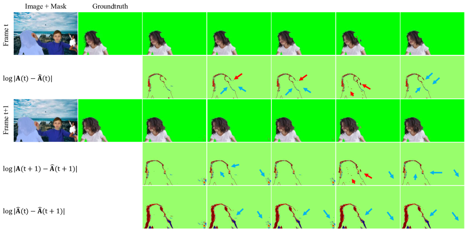
Conv-GRU	Single		✓
	Bidirectional			✓	✓	✓
Fusion	$\mathbf{\hat{A}}^{f}$				✓	✓
	$\mathbf{\hat{A}}^{b}$					✓

Figure 18: The effectiveness of different temporal components on the medium level of V-HIM60. Conv-GRU can improve the result a bit, but not perfect. Our proposed fusion strategy improves the output in both foreground and background regions. The table below denotes temporal components for each column. Red, blue arrows indicate the errors and improvements in comparison with the result without any temporal module. We also visualize the error to the groundtruth ($\log|\mathbf{A}-\mathbf{\hat{A}}|$) and the difference between consecutive predictions($\log|\mathbf{\hat{A}}-\mathbf{\hat{A}}|$). The color-coded map (min-max range) to illustrate differences between consecutive frames is . (Best viewed in color and digital zoom).

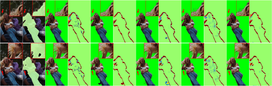
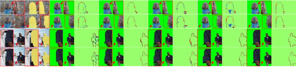
Frame	Input mask	$\hat{\mathbf{A}}$	$\log\mathopen{}\left|\Delta_{\hat{\mathbf{A}}}\mathclose{}\right|$	$\hat{\mathbf{A}}$	$\log\mathopen{}\left|\Delta_{\hat{\mathbf{A}}}\mathclose{}\right|$	$\hat{\mathbf{A}}$	$\log\mathopen{}\left|\Delta_{\hat{\mathbf{A}}}\mathclose{}\right|$	$\hat{\mathbf{A}}$	$\log\mathopen{}\left|\Delta_{\hat{\mathbf{A}}}\mathclose{}\right|$	$\hat{\mathbf{A}}$	$\log\mathopen{}\left|\Delta_{\hat{\mathbf{A}}}\mathclose{}\right|$
		$\underbrace{\hskip 73.97733pt}_{\begin{subarray}{c}\vspace{-5.0mm}\end{subarray}\hbox{\pagecolor{white}~{}~{}InstMatt~{}~{}}}$		$\underbrace{\hskip 73.97733pt}_{\begin{subarray}{c}\vspace{-5.0mm}\end{subarray}\hbox{\pagecolor{white}~{}~{}SparseMat~{}~{}}}$		$\underbrace{\hskip 73.97733pt}_{\begin{subarray}{c}\vspace{-5.0mm}\end{subarray}\hbox{\pagecolor{white}~{}~{}MGM-TCVOM~{}~{}}}$		$\underbrace{\hskip 73.97733pt}_{\begin{subarray}{c}\vspace{-5.0mm}\end{subarray}\hbox{\pagecolor{white}~{}~{}MGM${}^{\star}$-TCVOM~{}~{}}}$		$\underbrace{\hskip 73.97733pt}_{\begin{subarray}{c}\vspace{-5.0mm}\end{subarray}\hbox{\pagecolor{white}~{}~{}Ours~{}~{}}}$

Figure 19: Highlighted detail and consistency on natural video outputs. To watch the full videos, please check our website. We present the foreground extracted and the difference to the previous frame output for each model. The color-coded map (min-max range) to illustrate differences between consecutive frames is . Red arrows indicate the zoom-in region in the red square. (Best viewed in color and digital zoom).

References

- Adobe [2023] Adobe. Adobe premiere. https://www.adobe.com/products/premiere.html, 2023.
- Apple [2023] Apple. Cutouts object ios 16. https://support.apple.com/en-hk/102460, 2023.
- Ballas et al. [2015] Nicolas Ballas, Li Yao, Chris Pal, and Aaron Courville. Delving deeper into convolutional networks for learning video representations. arXiv preprint arXiv:1511.06432, 2015.
- Berman et al. [2000] Arie Berman, Arpag Dadourian, and Paul Vlahos. Method for removing from an image the background surrounding a selected object, 2000. US Patent 6,134,346.
- Chen et al. [2022a] Guowei Chen, Yi Liu, Jian Wang, Juncai Peng, Yuying Hao, Lutao Chu, Shiyu Tang, Zewu Wu, Zeyu Chen, Zhiliang Yu, et al. Pp-matting: high-accuracy natural image matting. arXiv preprint arXiv:2204.09433, 2022a.
- Chen et al. [2022b] Xiangguang Chen, Ye Zhu, Yu Li, Bingtao Fu, Lei Sun, Ying Shan, and Shan Liu. Robust human matting via semantic guidance. In ACCV, 2022b.
- Cheng et al. [2022] Bowen Cheng, Ishan Misra, Alexander G Schwing, Alexander Kirillov, and Rohit Girdhar. Masked-attention mask transformer for universal image segmentation. In CVPR, 2022.
- Cheng and Schwing [2022] Ho Kei Cheng and Alexander G Schwing. Xmem: Long-term video object segmentation with an atkinson-shiffrin memory model. In ECCV, 2022.
- Cho et al. [2016] Donghyeon Cho, Yu-Wing Tai, and Inso Kweon. Natural image matting using deep convolutional neural networks. In ECCV, 2016.
- Contributors [2022] Spconv Contributors. Spconv: Spatially sparse convolution library. https://github.com/traveller59/spconv, 2022.
- Forte and Pitié [2020] Marco Forte and François Pitié. , , alpha matting. arXiv preprint arXiv:2003.07711, 2020.
- Google [2023] Google. Magic editor in google pixel 8. https://pixel.withgoogle.com/Pixel_8_Pro/use-magic-editor, 2023.
- He et al. [2016] Kaiming He, Xiangyu Zhang, Shaoqing Ren, and Jian Sun. Deep residual learning for image recognition. In CVPR, 2016.
- He et al. [2017] Kaiming He, Georgia Gkioxari, Piotr Dollár, and Ross Girshick. Mask r-cnn. In ICCV, 2017.
- Hebborn et al. [2017] Anna Katharina Hebborn, Nils Höhner, and Stefan Müller. Occlusion matting: realistic occlusion handling for augmented reality applications. In 2017 IEEE International Symposium on Mixed and Augmented Reality (ISMAR). IEEE, 2017.
- Hou and Liu [2019] Qiqi Hou and Feng Liu. Context-aware image matting for simultaneous foreground and alpha estimation. In ICCV, 2019.
- Huang and Lee [2023] Wei-Lun Huang and Ming-Sui Lee. End-to-end video matting with trimap propagation. In CVPR, 2023.
- Huynh et al. [2021] Chuong Huynh, Anh Tuan Tran, Khoa Luu, and Minh Hoai. Progressive semantic segmentation. In CVPR, 2021.
- Huynh et al. [2023] Chuong Huynh, Yuqian Zhou, Zhe Lin, Connelly Barnes, Eli Shechtman, Sohrab Amirghodsi, and Abhinav Shrivastava. Simpson: Simplifying photo cleanup with single-click distracting object segmentation network. In CVPR, 2023.
- Imambi et al. [2021] Sagar Imambi, Kolla Bhanu Prakash, and GR Kanagachidambaresan. Pytorch. Programming with TensorFlow: Solution for Edge Computing Applications, 2021.
- Ke et al. [2022a] Lei Ke, Henghui Ding, Martin Danelljan, Yu-Wing Tai, Chi-Keung Tang, and Fisher Yu. Video mask transfiner for high-quality video instance segmentation. In ECCV, 2022a.
- Ke et al. [2022b] Zhanghan Ke, Jiayu Sun, Kaican Li, Qiong Yan, and Rynson WH Lau. Modnet: Real-time trimap-free portrait matting via objective decomposition. In AAAI, 2022b.
- Kirillov et al. [2023] Alexander Kirillov, Eric Mintun, Nikhila Ravi, Hanzi Mao, Chloe Rolland, Laura Gustafson, Tete Xiao, Spencer Whitehead, Alexander C. Berg, Wan-Yen Lo, Piotr Dollar, and Ross Girshick. Segment anything. In ICCV, 2023.
- Lee and Wu [2011] Philip Lee and Ying Wu. Nonlocal matting. In CVPR, 2011.
- Levin et al. [2007] Anat Levin, Dani Lischinski, and Yair Weiss. A closed-form solution to natural image matting. IEEE TPAMI, 30(2), 2007.
- Li et al. [2021a] Jizhizi Li, Sihan Ma, Jing Zhang, and Dacheng Tao. Privacy-preserving portrait matting. In ACM MM, 2021a.
- Li et al. [2021b] Jizhizi Li, Jing Zhang, and Dacheng Tao. Deep automatic natural image matting. In IJCAI, 2021b.
- Li et al. [2022a] Jiachen Li, Vidit Goel, Marianna Ohanyan, Shant Navasardyan, Yunchao Wei, and Humphrey Shi. Vmformer: End-to-end video matting with transformer. arXiv preprint arXiv:2208.12801, 2022a.
- Li et al. [2022b] Jizhizi Li, Jing Zhang, Stephen J Maybank, and Dacheng Tao. Bridging composite and real: towards end-to-end deep image matting. IJCV, 2022b.
- Li et al. [2024] Jiachen Li, Roberto Henschel, Vidit Goel, Marianna Ohanyan, Shant Navasardyan, and Humphrey Shi. Video instance matting. In WACV, 2024.
- Li and Lu [2020] Yaoyi Li and Hongtao Lu. Natural image matting via guided contextual attention. In AAAI, 2020.
- Lin et al. [2023] Chung-Ching Lin, Jiang Wang, Kun Luo, Kevin Lin, Linjie Li, Lijuan Wang, and Zicheng Liu. Adaptive human matting for dynamic videos. In CVPR, 2023.
- Lin et al. [2021] Shanchuan Lin, Andrey Ryabtsev, Soumyadip Sengupta, Brian L Curless, Steven M Seitz, and Ira Kemelmacher-Shlizerman. Real-time high-resolution background matting. In CVPR, 2021.
- Lin et al. [2022] Shanchuan Lin, Linjie Yang, Imran Saleemi, and Soumyadip Sengupta. Robust high-resolution video matting with temporal guidance. In WACV, 2022.
- Lin et al. [2014] Tsung-Yi Lin, Michael Maire, Serge Belongie, James Hays, Pietro Perona, Deva Ramanan, Piotr Dollár, and C Lawrence Zitnick. Microsoft coco: Common objects in context. In ECCV, 2014.
- Liu et al. [2015] Baoyuan Liu, Min Wang, Hassan Foroosh, Marshall Tappen, and Marianna Pensky. Sparse convolutional neural networks. In CVPR, 2015.
- Lu et al. [2019] Hao Lu, Yutong Dai, Chunhua Shen, and Songcen Xu. Indices matter: Learning to index for deep image matting. In CVPR, 2019.
- Oh et al. [2019] Seoung Wug Oh, Joon-Young Lee, Ning Xu, and Seon Joo Kim. Video object segmentation using space-time memory networks. In ICCV, 2019.
- Park et al. [2023] Kwanyong Park, Sanghyun Woo, Seoung Wug Oh, In So Kweon, and Joon-Young Lee. Mask-guided matting in the wild. In CVPR, 2023.
- Pham et al. [2022] Khoi Pham, Kushal Kafle, Zhe Lin, Zhihong Ding, Scott Cohen, Quan Tran, and Abhinav Shrivastava. Improving closed and open-vocabulary attribute prediction using transformers. In ECCV, 2022.
- Pham et al. [2024] Khoi Pham, Chuong Huynh, and Abhinav Shrivastava. Composing object relations and attributes for image-text matching. In CVPR, 2024.
- Phung et al. [2024] Quynh Phung, Songwei Ge, and Jia-Bin Huang. Grounded text-to-image synthesis with attention refocusing. In CVPR, 2024.
- Russakovsky et al. [2015] Olga Russakovsky, Jia Deng, Hao Su, Jonathan Krause, Sanjeev Satheesh, Sean Ma, Zhiheng Huang, Andrej Karpathy, Aditya Khosla, Michael Bernstein, et al. Imagenet large scale visual recognition challenge. IJCV, 2015.
- Sengupta et al. [2020] Soumyadip Sengupta, Vivek Jayaram, Brian Curless, Steven M Seitz, and Ira Kemelmacher-Shlizerman. Background matting: The world is your green screen. In CVPR, 2020.
- Seong et al. [2022] Hongje Seong, Seoung Wug Oh, Brian Price, Euntai Kim, and Joon-Young Lee. One-trimap video matting. In ECCV, 2022.
- Shen et al. [2016] Xiaoyong Shen, Xin Tao, Hongyun Gao, Chao Zhou, and Jiaya Jia. Deep automatic portrait matting. In ECCV, 2016.
- Sun et al. [2021a] Yanan Sun, Chi-Keung Tang, and Yu-Wing Tai. Semantic image matting. In CVPR, 2021a.
- Sun et al. [2021b] Yanan Sun, Guanzhi Wang, Qiao Gu, Chi-Keung Tang, and Yu-Wing Tai. Deep video matting via spatio-temporal alignment and aggregation. In CVPR, 2021b.
- Sun et al. [2022] Yanan Sun, Chi-Keung Tang, and Yu-Wing Tai. Human instance matting via mutual guidance and multi-instance refinement. In CVPR, 2022.
- Sun et al. [2023] Yanan Sun, Chi-Keung Tang, and Yu-Wing Tai. Ultrahigh resolution image/video matting with spatio-temporal sparsity. In CVPR, 2023.
- Vaswani et al. [2017] Ashish Vaswani, Noam Shazeer, Niki Parmar, Jakob Uszkoreit, Llion Jones, Aidan N Gomez, Łukasz Kaiser, and Illia Polosukhin. Attention is all you need. NeurIPS, 30, 2017.
- Wang et al. [2021] Tiantian Wang, Sifei Liu, Yapeng Tian, Kai Li, and Ming-Hsuan Yang. Video matting via consistency-regularized graph neural networks. In ICCV, 2021.
- Wang et al. [2023] Yumeng Wang, Bo Xu, Ziwen Li, Han Huang, Cheng Lu, and Yandong Guo. Video object matting via hierarchical space-time semantic guidance. In WACV, 2023.
- Xu et al. [2017] Ning Xu, Brian Price, Scott Cohen, and Thomas Huang. Deep image matting. In CVPR, 2017.
- Yang et al. [2021] Zongxin Yang, Yunchao Wei, and Yi Yang. Associating objects with transformers for video object segmentation. NeurIPS, 2021.
- Yu et al. [2021] Qihang Yu, Jianming Zhang, He Zhang, Yilin Wang, Zhe Lin, Ning Xu, Yutong Bai, and Alan Yuille. Mask guided matting via progressive refinement network. In CVPR, 2021.
- Zhang et al. [2021] Yunke Zhang, Chi Wang, Miaomiao Cui, Peiran Ren, Xuansong Xie, Xian-Sheng Hua, Hujun Bao, Qixing Huang, and Weiwei Xu. Attention-guided temporally coherent video object matting. In ACM MM, 2021.