ST-MambaSync: The Confluence of Mamba Structure and Spatio-Temporal Transformers for Precipitous Traffic Prediction

Abstract

Balancing accuracy with computational efficiency is paramount in machine learning, particularly when dealing with high-dimensional data, such as spatial-temporal datasets. This study introduces ST-MambaSync, an innovative framework that integrates a streamlined attention layer with a simplified state-space layer. The model achieves competitive accuracy in spatial-temporal prediction tasks. We delve into the relationship between attention mechanisms and the Mamba component, revealing that Mamba functions akin to attention within a residual network structure. This comparative analysis underpins the efficiency of state-space models, elucidating their capability to deliver superior performance at reduced computational costs.

[first]organization=Business Analytics,addressline=University of Sydney, city=Sydney, postcode=2006, state=NSW, country=Australia

[second]organization=College of Management and Economics,addressline=Tianjin University, city=Tianjin, postcode=300072, country=China . [second]organization=ITLS, , addressline=University of Sydney, city=Sydney, postcode=2006, state=NSW, country=Australia

1 Introduction

Traffic prediction is essential for urban planning, road safety, and efficiency, significantly influencing the management of traffic flows, reduction of congestion, and the proactive deployment of resources to address potential disruptions. Accurate traffic forecasts allow for better traffic management and routing, which can reduce the risk of accidents and congestion. If commuters are informed about potential delays, they can take alternative routes or adjust their travel times, enhancing road safety and convenience. However, the challenge lies in achieving high accuracy but with low computational cost in both short-term (accurate predictions within a 1 to 5-minute timeframe) (Nagy and Simon, 2018) and especially in long-term (forecasting window to more than 30 minutes) prediction tasks.

Traditional approaches to traffic flow prediction, such as historical average (HA) (Smith, 1995), autoregressive integrated moving average (ARIMA) (Kumar and Vanajakshi, 2015), and support-vector regression (SVR) models (Wu et al., 2004), have laid the foundation for this field of study. While these models have provided valuable insights, their inherent simplicity and linear nature often limit their capacity to fully capture the nonlinear and high-dimensional relationships present in traffic data. As a result, the accuracy of these models may be compromised, particularly in complex and dynamic traffic scenarios.

In recent years, the traffic flow prediction field has witnessed significant advancements with the introduction of deep learning techniques. While models such as Convolutional Neural Networks (CNNs) (Sayed et al., 2023) and Recurrent Neural Networks (RNNs) have shown promise in capturing spatial and temporal dependencies, they are not without limitations. CNNs excel in processing spatial information but may struggle with capturing long-range temporal dependencies. On the other hand, RNNs, including Long Short-Term Memory (LSTM) and Gated Recurrent Unit (GRU) networks, have demonstrated success in modeling temporal dynamics. However, RNNs can face challenges in capturing very long-term dependencies due to the vanishing gradient problem, which can hinder their ability to effectively model long sequences. Additionally, the sequential nature of RNNs can limit their parallelization capabilities, leading to slower training and inference times compared to feed-forward architectures like CNNs.

Recent research has explored the potential of Transformer models, originally developed for natural language processing tasks, in traffic flow prediction. Transformers introduce a novel approach to capturing dependencies through self-attention mechanisms. By allowing the model to weigh the importance of different parts of the input data, Transformers can effectively model complex relationships without the sequential processing limitations of RNNs. This ability to capture long-range dependencies has shown promise in improving the accuracy of long-term traffic flow predictions.

However, Transformer models come with their own set of challenges. The self-attention mechanism, while powerful, can be computationally expensive, particularly when dealing with large-scale traffic networks and long historical data sequences. The computational complexity of Transformers grows quadratically with the input sequence length, leading to slower training and testing phases compared to other models. Additionally, the high computational cost associated with Transformers can hinder their practical application in long-term traffic management systems, where swift predictions are crucial.

The Selective State of Space model (which is the so-called Mamba) (Gu and Dao, 2024) has a distinctive advantage in its capability to provide high-accuracy forecasts with reduced computational demands. This efficiency is particularly valuable in both short-term and long-term traffic management scenarios, where swift, reliable predictions are essential for effective congestion control, route optimization, and traffic flow regulation.

This paper introduces the Spatial-Temporal Selective State Space Model (ST-SSMs), an innovative framework for efficient and accurate traffic flow prediction. The ST-SSMs model seamlessly integrates spatial and temporal data through an ST-Mixer, eliminating the need to treat these data types separately. The integrated data is then processed by the ST-Mamba block, which excels at identifying and modeling the most significant patterns and dependencies in traffic data over extended periods.

A key feature of the ST-SSMs model is its ability to effectively and accurately process long-term traffic flow predictions by leveraging the strengths of Selective State Space Models (SSMs) within the ST-Mamba block. This makes ST-SSMs particularly effective for long-term analysis without compromising precision. As a state-of-the-art model designed specifically for non-graph-based Spatial-Temporal (ST) data, ST-SSMs introduce a new paradigm in traffic flow prediction. By utilizing the specially designed ST-Mamba block, the ST-SSMs model offers an advanced alternative to existing approaches, delivering more precise and faster forecasts of long-term traffic flow dynamics that reflect the intricate interplay of spatial and temporal factors.

To the best of our knowledge, this paper presents the pioneering integration of a selective state-of-space model and attention that used in spatial temporal data and proves that mamba is a kind of attention with residual network. The key contributions of this research can be succinctly summarized as follows:

• This study introduces the integration of Mamba and attention blocks for handling spatial-temporal data in both real-time and long-term traffic forecasting tasks.

• We provide theoretical proof that the Mamba can be conceptualized as an attention mechanism within a ResNet framework.

• Through extensive experiments on real-world traffic datasets, we demonstrate the superior performance of our model compared to state-of-the-art benchmarks. Our approach achieves significant improvements in accuracy while reducing computation complexity.

2 Literature Review

3 Prelimanary

3.1 Attention

The self-attention mechanism, originally conceived for natural language processing (NLP), enriches the representation of feature data by revealing the underlying ’self-attention’ within the data set. Beginning with the input $X\in\mathbb{R}^{N\times d}$, the mechanism constructs queries ($Q$), keys ($K$), and values ($V$) via transformation matrices:

$$Q=XW_{Q},\quad K=XW_{K},\quad V=XW_{V},$$ (1)

where $W_{Q}\in\mathbb{R}^{d\times d_{q}}$, $W_{K}\in\mathbb{R}^{d\times d_{k}}$, $W_{V}\in\mathbb{R}^{d\times d_{v}}$ are weight matrices that are learned, and $d_{q}=d_{k}=d_{v}=d_{0}$ for simplicity.

Attention scores are computed by the scaled dot-product of queries and keys:

$$A=\frac{{Q}{K}^{\top}}{\sqrt{d_{k}}},$$ (2)

where scaling by $\sqrt{d_{k}}$ provides numerical stability.

The attention scores $A$ are normalized using the softmax function to obtain the attention weights $O$:

$$O=\text{softmax}(A).$$ (3)

The final representation $Y$ emerges as the weighted sum of the values:

$$Y=OV.$$ (4)

Multi-head attention leverages multiple ’heads’ of $Q$, $K$, and $V$ to explore different representation subspaces, creating a rich, integrated output.

Remark 1: We standardize $d_{q}=d_{k}=d_{v}=d_{0}$ to ensure uniform dimensions across the attention mechanism’s architecture.

3.2 State of Space Model

The state-space representation of a continuous-time linear time-invariant system can be described by the following differential equations:

$$\dot{h}(t) =Ah(t)+Bu(t)$$

$$y(t) =Ch(t)+Du(t)$$

The solution to the state equation over a time interval can be given by:

$$h(t_{b}) =e^{A(t_{b}-t_{a})}h(t_{a})+\int_{t_{a}}^{t_{b}}e^{A(t_{b}-\tau)}B(\tau)u(\tau)\,d\tau$$ (5)

In discrete time-steps, the state at step $b$ is given by:

$$h_{b} =e^{A(\Delta_{a}+\dots+\Delta_{b-1})}\left(h_{a}+\sum_{i=a}^{b-1}B_{i}u_{i}e^{-A(\Delta_{a}+\dots+\Delta_{i})}\Delta_{i}\right)$$ (6)

For the transition from state $h_{a}$ to state $h_{a+1}$, the following discrete update can be used:

$$h_{a+1} =e^{A\Delta_{a}}\left(h_{a}+B_{a}u_{a}e^{-A\Delta_{a}}\right)$$ (7)

$$=e^{A\Delta_{a}}h_{a}+B_{a}u_{a}$$ (8)

$$=\hat{A}_{a}h_{a}+\hat{B}_{a}u_{a}$$ (9)

4 Method

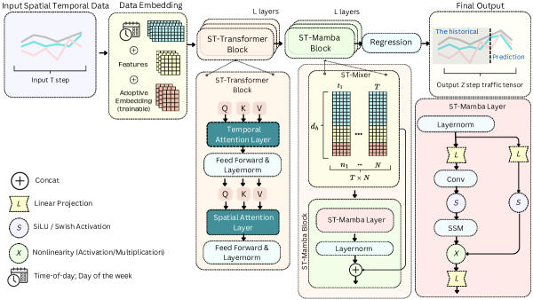
Figure 1: Caption

4.1 Data Embedding

To encapsulate and reflect the dynamic temporal patterns present within the traffic data, we utilized a modifiable data embedding layer that processes the sequential input $\mathbf{X}_{t-M+1:t}$. Through the application of a dense neural layer, we extract the intrinsic feature embedding $\mathbf{Z}_{f}\in\mathbb{R}^{M\times N\times d_{e}}$:

$$\mathbf{Z}_{f}=\text{Dense}(\mathbf{X}_{t-M+1:t})$$ (10)

Here, $d_{e}$ signifies the dimension of the embedded features, and $\text{Dense}(\cdot)$ represents the applied dense layer. Furthermore, we introduce a parameterized dictionary for the embedding of weekdays $\mathbf{Z}_{w}\in\mathbb{R}^{7\times d_{e}}$ and another for the embedding of distinct times of the day $\mathbf{Z}_{h}\in\mathbb{R}^{288\times d_{e}}$, encapsulating the cyclical nature of weeks with 7 days and days with 288 time intervals. With $\mathbf{W}_{t}\in\mathbb{R}^{M}$ representing the weekday index and $\mathbf{H}_{t}\in\mathbb{R}^{M}$ representing the time-of-day index over the period from $t-M+1$ to $t$, we map these indices to their respective embeddings, yielding the weekday embedded features $\mathbf{Z}_{w_{t}}\in\mathbb{R}^{M\times d_{e}}$ and time-of-day embedded features $\mathbf{Z}_{h_{t}}\in\mathbb{R}^{M\times d_{e}}$. The combination and expansion of these embeddings generate the cyclical feature embedding $\mathbf{Z}_{c}\in\mathbb{R}^{M\times N\times 2d_{e}}$, which is utilized to incorporate periodic patterns into the traffic data.

Considering the rhythmic progression of time and the interlinked nature of traffic events, traffic sensors yield data with unique temporal traits. To address the need for a uniform approach to encapsulate these spatio-temporal dynamics, a shared spatio-temporal adaptive embedding, $\mathbf{Z}_{s}\in\mathbb{R}^{M\times N\times d_{s}}$, is put forth. This embedding is initialized utilizing Xavier uniform initialization, a technique that primes the model’s weights to avoid excessively large or small gradients initially, and thereafter, it is treated as a model parameter.

The integration of the aforesaid embeddings results in a hidden spatio-temporal representation $\mathbf{Z}\in\mathbb{R}^{M\times N\times d_{h}}$:

$$\mathbf{Z}=\textbf{Concatenate}(\mathbf{Z}_{f};\mathbf{Z}_{c};\mathbf{Z}_{s})$$ (11)

In this equation, the concatenation operation is denoted by a comma, and the dimension of the hidden representation $d_{h}$ is computed as $3d_{e}+d_{s}$.

4.2 Spatial Temporal Transformer (ST-Transformer Block)

We utilize standard transformers along both temporal and spatial dimensions to understand complex traffic interactions. Given a hidden spatio-temporal matrix $\mathbf{Z}\in\mathbb{R}^{T\times N\times d_{h}}$, where $T$ is the number of frames and $N$ represents spatial nodes, we derive the query, key, and value matrices using temporal transformer layers as follows:

$$\mathbf{Q}^{(te)} =\mathbf{Z}\mathbf{W}_{Q}^{(te)},$$ (12)

$$\mathbf{K}^{(te)} =\mathbf{Z}\mathbf{W}_{K}^{(te)},$$ (13)

$$\mathbf{V}^{(te)} =\mathbf{Z}\mathbf{W}_{V}^{(te)},$$ (14)

where $\mathbf{W}_{Q}^{(te)},\mathbf{W}_{K}^{(te)},\mathbf{W}_{V}^{(te)}\in\mathbb{R}^{d_{h}\times d_{h}}$ are learnable parameters. The self-attention scores are computed as:

$$\mathbf{A}^{(te)}=\text{Softmax}\left(\frac{\mathbf{Q}^{(te)}(\mathbf{K}^{(te)})^{\top}}{\sqrt{d_{h}}}\right),$$ (15)

capturing temporal connections across different spatial nodes. The output of the temporal transformer, $\mathbf{Z}^{(te)}\in\mathbb{R}^{T\times N\times d_{h}}$, is then obtained as:

$$\mathbf{Z}^{(te)}=\mathbf{A}^{(te)}\mathbf{V}^{(te)}.$$ (16)

In a similar fashion, the spatial transformer layer functions by processing $\mathbf{Z}^{(te)}$ through self-attention (following the same equations) to produce $\mathbf{Z}^{(sp)}\in\mathbb{R}^{T\times N\times d_{h}}$. Important enhancements include layer normalization, residual connections, and a multi-head mechanism.

4.3 Spatial Temporal Selective State of Spatial (ST-Mamba block)

As depicted in Figure 1, following the adaptive ST-Transformer block, our framework employs a simplified ST-Mamba block. This block features an ST-Mamba layer designed to reduce computational costs and to enhance long-term memory. To feed the input to ST-Mamba block, we employ a tersor reshape named as ST-mixer as:

ST-mixer

To effectively blend spatial and temporal data, the ST-SSMs utilize tensor reshaping, as detailed in Figure 1, to transform tensor $\mathbf{Z}^{(sp)}$ into matrix $\mathbf{\bar{X}}$. This transformation involves aligning and concatenating the tensor slices across each time step $t$ as follows:

$$\mathbf{\bar{X}}=\text{reshape}(\mathbf{Z}^{(sp)}).$$ (17)

Through this reshaping, we obtain a new embedding $\mathbf{\bar{X}}$ in $\mathbb{R}^{\mathcal{T}\times d_{h}}$, where $\mathcal{T}$ encapsulates the total temporal length $T\times N$, representing the spatial dimension. This reshaping facilitates the unified processing of spatial and temporal information, thereby capturing complex patterns in the data more effectively.

4.3.1 ST-Mamba Layer

The ST-Mamba layer, described , leverages the discretization of continuous state-space models (SSM) as in Section 3.2. We represent the input to the ST-Mamba block as $\mathcal{H}$, where $\mathcal{H}=\text{LayerNorm}(\mathbf{\bar{X}})$. This representation is fed into the selective state-space model (SSM) layer for further processing. The linear transformation within the layer results in:

$$\mathbf{U}=Linear(\mathcal{H}),$$ (18)

which $\mathbf{U}\in\mathbb{R}^{d_{h}\times\mathcal{T}}$ denotes the hidden representation of the latent state at each iteration step $k$. The goal is to compute the output $\mathbf{Y}\in\mathbb{R}^{d_{inner}\times\mathcal{T}}$, and subsequently project $\mathbf{Y}$ back to the input shape $\mathcal{T}\times d_{h}$.

Parameter Initialization

The initialization of ST-SSM parameters is crucial for the functionality of the layer:

• $\mathbf{A}\in\mathbb{R}^{d_{inner}\times d_{state}}$: Structured state transition matrix initialized using HiPPO to capture long-range dependencies.

• $\mathbf{B}\in\mathbb{R}^{d_{state}\times\mathcal{T}}$: Computed as $\mathbf{B}=s_{B}(\mathbf{U})$, where $s_{B}(\cdot)$ is a learnable linear projection.

• $\mathbf{C}\in\mathbb{R}^{d_{state}\times\mathcal{T}}$: Output projection matrix, computed as $\mathbf{C}=s_{C}(\mathbf{U})$, where $s_{C}(\cdot)$ is another learnable linear projection.

• $\mathbf{D}\in\mathbb{R}^{d_{inner}}$: Learnable parameter that allows bypassing the state transformation for direct input-to-output information transfer.

• $\Delta\in\mathbb{R}^{\mathbb{R}^{d_{state}\times\mathcal{T}}}$: Step size parameter calculated using $\Delta=\tau_{\Delta}(\text{Parameter}+s_{\Delta}(\mathbf{U}))$, with $\tau_{\Delta}$ as the softplus function and $s_{\Delta}(\cdot)$ as a linear projection.

Discretization and Output Computation

Discretizing the continuous-time parameters to obtain discrete-time SSM parameters involves:

$$\mathbf{\tilde{A}} =\exp(\Delta\mathbf{A}),$$ (19)

$$\mathbf{\tilde{B}} =\mathbf{A}^{-1}(\exp(\Delta\mathbf{A})-\mathbf{I})\mathbf{B},$$ (20)

where $\exp(\cdot)$ denotes the matrix exponential, and $\mathbf{I}$ is the identity matrix of appropriate size. The discrete-time matrices, $\mathbf{\tilde{A}}$ and $\mathbf{\tilde{B}}$, are then used in the recurrence of the selective ST-Mamba layer:

$$\mathbf{H}_{k} =\mathbf{\tilde{A}}\odot\mathbf{H}_{k-1}+\mathbf{\tilde{B}}\odot\mathbf{U}_{k},$$ (21)

$$\mathbf{Y}_{k} =\mathbf{C}\odot\mathbf{H}_{k}+\mathbf{D}\odot\mathbf{U}_{k},$$ (22)

where $\odot$ represents the Hadamard product. The process iterates over each step from $k=1$ to $\mathcal{T}$, ensuring the transformation of each step’s data through the SSM layer. The final output $\mathbf{Y}$ is shaped into $\mathbb{R}^{\mathcal{T}\times d_{inner}}$ to match the input dimensions.

4.3.2 ST-Mamba block and Regression Layer

Normalization Layer

Within the ST-Mamba block, the normalization of layers is crucial for improving the training’s stability and efficiency. Specifically, consider an input matrix $\mathbf{Y}$ with dimensions $\mathbb{R}^{\mathcal{T}\times d_{h}}$, where $\mathcal{T}$ represents the sequence length or sample count, and $d_{h}$ indicates the features’ dimensional space. The normalization process is described by:

$$\text{Normalization}(\mathbf{Y})=\gamma\odot\frac{\mathbf{Y}-\mu}{\sqrt{\sigma^{2}+\epsilon}}+\beta.$$ (23)

In this formula, $\mu$ and $\sigma^{2}$ are the mean and variance computed along the features’ dimension $d_{h}$, resulting in vectors of size $\mathcal{T}\times 1$. The scale ($\gamma$) and shift ($\beta$) parameters, each sized $1\times d_{h}$, are adjustable, optimizing the normalization’s impact. This process ensures stability in the model’s learning phase while allowing the reintegration of the original activations distribution if it improves model performance. The addition of $\epsilon$, a small constant, prevents any division by zero, maintaining numerical stability. Through layer normalization, the model effectively reduces internal covariate shift, enhancing training speed and boosting overall deep learning performance.

Regression Layer

As in Referring to Figure 1, the output from the ST-Mamba block passes through a normalization step before reaching the regression layer, which is structured as follows:

$$\mathbf{\bar{Y}} =\text{Normalization}(\mathbf{Y})+\mathbf{\bar{X}}$$ (24)

$$\mathcal{Y} =FC(\mathbf{\bar{Y}})$$ (25)

In this configuration, $FC(\cdot)$ denotes the fully connected layer that processes the normalized data. The resultant $\mathcal{Y}$, existing within the dimensional space $\mathbb{R}^{Z\times N\times d}$, marks the culmination of the process. This structured approach showcases how architectural enhancements are designed to improve the training of deep networks and accurately interpret complex, multi-dimensional datasets.

4.4 Mamba is a kind of Attention in ResNet

Attention can be seen as a kind of linear regression but not used for prediction. Given a set of data $\{(x_{i},y_{i})\}_{i=1}^{N}$ with $x_{i}\in\mathbb{R}^{d}$ and $y_{i}\in\mathbb{R}$, for a linear model:

$$y =x_{i}^{T}\omega+b,$$ (26)

for simplicity, set $b=0$ or absorb $b$ into $\omega$. The data matrix can be denoted as:

$$X=\begin{bmatrix}x_{1}^{T}\\ \vdots\\ x_{N}^{T}\end{bmatrix}\in\mathbb{R}^{N\times d},\quad\mathbf{y}=\begin{bmatrix}y_{1}\\ \vdots\\ y_{N}\end{bmatrix}.$$ (27)

The least squares solution is given by:

$$\hat{\omega}=(X^{T}X)^{-1}X^{T}\mathbf{y}.$$ (28)

For model prediction on the training data with the least squares solution, we can write the formulation as:

$$\hat{y}=X\hat{\omega}=X(X^{T}X)^{-1}X^{T}\mathbf{y},$$ (29)

With a the given set of data $\{(x_{i},y_{i})\}_{i=1}^{N}$, for find the solution of $\hat{y}_{1}$, it can be written as:

$$\hat{y}_{1} =a_{11}y_{1}+a_{12}y_{2}+\dots+a_{1N}y_{N},$$ (30)

$$a_{ij} =x_{i}^{T}(X^{T}X)^{-1}x_{j},$$ (31)

in this case, the $a_{ij}$s are analogous to the attention scores, which are $QK^{T}$. The model prediction $\hat{y}_{1}$ at $x_{1}$ is the ’similarity’ average over all the training values.

For a new data point $x^{\prime}$, the prediction $\hat{y}(x^{\prime})$ by the model is given by:

$$\hat{y}(x^{\prime})=x^{\prime}(X^{T}X)^{-1}X^{T}\mathbf{y}.$$ (32)

This can be interpreted as the weighted sum of the training data targets, where the weights are the similarities between the new data point and the training data points. Here, $x^{\prime T}(X^{T}X)^{-1}X^{T}$ can be seen as $QK^{T}$, and $\mathbf{y}$ is the $V$.

In the context of commonly used linear attention on data, given data $X\in\mathbb{R}^{N\times d}$, attention can be formulated as:

$$\text{attn}(X)=XW_{Q}W_{K}^{T}X^{T}XW_{V}.$$ (33)

Now, we move to the discrete update on SSM, which is shown in the following equation (assumed to be Equation 7), treated as the attention score $a_{ij}$, representing the solution or $Q\cdot V$:

$$h_{a+1} =e^{A\Delta_{a}}\left(h_{a}+B_{a}u_{a}e^{-A\Delta_{a}}\Delta A\right)$$ (34)

$$=e^{A\Delta_{a}}h_{a}+B_{a}u_{a}e^{-A\Delta_{a}}\Delta Ae^{A\Delta_{a}}$$ (35)

Here, we set $Q_{m}=B_{a}$, $K_{m}=u_{a}$, the weight $W=e^{A\Delta_{a}}$, and the trainable parameter $\beta=\Delta A$. Thus, it can be rewritten as:

$$h_{a+1}=Wh+Q_{m}K_{m}W^{-1}\beta.$$ (36)

For each discrete update, the SSMs are actually finding an attention score for each of the inputs $u_{a}$ and a learnable linear projection of the input $u_{a}$ (denoted as $B_{a}$).

To find the final results, we define $V_{m}$ as $C_{a}$, representing the values in the attention mechanism, and then:

$$y=W^{-1}\left(Q_{m}K_{m}^{T}\right)V_{m}+WV_{m}\beta h_{a+1}.$$ (37)

The first term resembles the attention mechanism, capturing the weighted importance of different inputs. The second term incorporates the updated hidden state, structured analogously to a Residual Network (ResNet), where the hidden state is updated by adding a transformed version of itself.

4.5 The iteration expression on ST-MambaSync

In ST-MambaSync, the embedded input of $\mathbf{Z}$ first goes through with 1 attention layer and then out it through an ST-Mamba Layer. To have a clear view for the inner iteration, we can formulate it as:

$$\textbf{attn}(\mathbf{Z})=$$ (38)

5 Experiment

5.1 Data Description and Baseline Models

Datasets

We test our method on six major traffic forecasting benchmarks, namely METR-LA, PEMS-BAY, PEMS03, PEMS04, PEMS07, and PEMS08, to verify its effectiveness. The datasets under consideration feature a time resolution of 5 minutes, which results in 12 data frames being recorded for every hour. The detail of the data is summarized in Table 1.

Table 1: Summary of Datasets.

Dataset	#Sensors (N)	#Timesteps	Time Range
METR-LA	207	34,272	03/2012 - 06/2012
PEMS-BAY	325	52,116	01/2017 - 05/2017
PEMS03	358	26,209	05/2012 - 07/2012
PEMS04	307	16,992	01/2018 - 02/2018
PEMS07	883	28,224	05/2017 - 08/2017
PEMS08	170	17,856	07/2016 - 08/2016

Baseline Models

In our comparative analysis, we evaluate the performance of our proposed approach against a comprehensive set of baselines within the traffic forecasting domain.

• Historical Index (HI) (Cui et al., 2021): serving as the conventional benchmark, reflecting standard industry practices.

Our examination extends to a series of Spatial-Temporal Graph Neural Networks (STGNNs)—including

• GWNet (Wu et al., 2020a): proposing a graph neural network framework that automatically extracts uni-directed relations among variables, addressing the limitation of existing methods in fully exploiting latent spatial dependencies in multivariate time series forecasting.

• DCRNN (Li et al., 2018): introducing the Diffusion Convolutional Recurrent Neural Network for traffic forecasting which captures both spatial and temporal dependencies.

• AGCRN (Bai et al., 2020): introducing adaptive modules to capture node-specific patterns and infer inter-dependencies among traffic series which provides fine-grained modeling of spatial and temporal dynamics in traffic data.

• STGCN (Yu et al., 2018): proposing a deep learning framework that integrates graph convolutions for spatial feature extraction and gated temporal convolutions for temporal feature extraction.

• GTS (Shang et al., 2021): proposing a method for forecasting multiple interrelated time series by learning a graph structure simultaneously with a Graph Neural Network (GNN) which addresses the limitations of a previous method.

• MTGNN (Wu et al., 2020b): proposing a graph neural network framework that automatically extracts uni-directed relations among variables which captures both spatial and temporal dependencies.

• GMAN (Zheng et al., 2020): introducing a graph-based deep learning model that incorporates spatial and temporal attention mechanisms to capture dynamic correlations among traffic sensors.

Recognizing the potential of Transformer-based models in time series forecasting, we particularly focus on:

• PDFormer (Jiang et al., 2023): introducing a traffic flow prediction model that captures dynamic spatial dependencies, long-range spatial dependencies, and the time delay in traffic condition propagation.

• STAEformer (Liu et al., 2023): proposing a spatio-temporal adaptive embedding that enhances the performance of vanilla transformers for traffic forecasting.

and which are adept at short-term traffic forecasting tasks. Additionally, we explore

• STNorm (Deng et al., 2021): leveraging spatial and temporal normalization modules to refine the high-frequency and local components underlying the raw data.

• STID (Shao et al., 2022): proposing an approach that addresses the indistinguishability of samples in both spatial and temporal dimensions by attaching spatial and temporal identity information to the input data.

Those diverse range of models allows for a robust validation of our proposed method’s capabilities.

5.2 Experiment Setup

Implementation

All experiments are conducted on a machine with the GPU RTX 3090(24GB) CPU 15. The dataset splits for PEMS-BAY, PEMS03, PEMS04, PEMS07, and PEMS08 are configured as follows: PEMS-BAY is segmented into training, validation, and test sets at a ratio of 7:1:2, while PEMS03, PEMS04, PEMS07, and PEMS08 follow a distribution ratio of 6:2:2. We set the embedding dimension ($d_{f}$) to 24 and the dimension of attention ($d_{a}$) to 80. The architecture includes three layers for both spatial and temporal transformers, with a head count of four. We define both the input and forecast horizon at 1 hour, corresponding to ${\color[rgb]{1,0,0}H}=Z=12$. For optimization, we employ the Adam optimizer, initiating with a learning rate of 0.001 that gradually decreases, and a batch size set at 16. To enhance training efficiency, an early stopping criterion is implemented, halting the process if validation error fails to improve over 30 consecutive iterations.

Metric

To evaluate the performance of traffic forecasting methods, three prevalent metrics are employed: the Mean Absolute Error (MAE), the Mean Absolute Percentage Error (MAPE), and the Root Mean Square Error (RMSE). These metrics offer a comprehensive view of model accuracy and error magnitude. They are defined as follows:

• MAE (Mean Absolute Error): quantifies the average magnitude of the errors in a set of predictions, without considering their direction. It’s calculated as:

  $$\text{MAE}=\frac{1}{n}\sum_{i=1}^{n}|\hat{y}_{i}-y_{i}|,$$

• MAPE (Mean Absolute Percentage Error): expresses the error as a percentage of the actual values, providing a normalization of errors that is useful for comparisons across datasets of varying scales. It’s given by:

  $$\text{MAPE}=\frac{1}{n}\sum_{i=1}^{n}\left|\frac{\hat{y}_{i}-y_{i}}{y_{i}}\right|\times 100,$$

• RMSE (Root Mean Square Error): measures the square root of the average squared differences between the predicted and actual values, offering a high penalty for large errors. This metric is defined as:

  $$\text{RMSE}=\sqrt{\frac{1}{n}\sum_{i=1}^{n}(\hat{y}_{i}-y_{i})^{2}}.$$

In these equations, $y=\{y_{1},y_{2},\ldots,y_{n}\}$ represents the set of ground-truth values, while $\hat{y}=\{\hat{y}_{1},\hat{y}_{2},\ldots,\hat{y}_{n}\}$ denotes the corresponding set of predicted values. Through the utilization of MAE, MAPE, and RMSE, a thorough evaluation of model performance in forecasting traffic conditions can be achieved, highlighting not just the average errors but also providing insights into the distribution and proportionality of these errors relative to true values.

Table 2: Performance comparison of models on PEMS datasets.

Model	PEMS03			PEMS04			PEMS07			PEMS08
	MAE	RMSE	MAPE	MAE	RMSE	MAPE	MAE	RMSE	MAPE	MAE	RMSE	MAPE
HI	$32.62$	$49.89$	30.60%	$42.35$	$61.66$	29.92%	$49.03$	$71.18$	22.75%	$36.66$	$50.45$	21.63%
GWNet	14.59	25.24	15.52%	$18.53$	$29.92$	12.89%	$20.47$	$33.47$	8.61%	$14.40$	$23.39$	9.21%
DCRNN	$15.54$	$27.18$	15.62%	$19.63$	$31.26$	13.59%	$21.16$	$34.14$	9.02%	$15.22$	$24.17$	10.21%
AGCRN	$15.24$	$26.65$	15.89%	$19.38$	$31.25$	13.40%	$20.57$	$34.40$	8.74%	$15.32$	$24.41$	10.03%
STGCN	$15.83$	$27.51$	16.13%	$19.57$	$31.38$	13.44%	$21.74$	$35.27$	9.24%	$16.08$	$25.39$	10.60%
GTS	$15.41$	$26.15$	15.39%	$20.96$	$32.95$	14.66%	$22.15$	$35.10$	9.38%	$16.49$	$26.08$	10.54%
MTGNN	$14.85$	$25.23$	14.55%	$19.17$	$31.70$	13.37%	$20.89$	$34.06$	9.00%	$15.18$	$24.24$	10.20%
STNorm	$15.32$	$25.93$	14.37%	$18.96$	$30.98$	12.69%	$20.50$	$34.66$	8.75%	$15.41$	$24.77$	9.76%
GMAN	$16.87$	$27.92$	18.23%	$19.14$	$31.60$	13.19%	$20.97$	$34.10$	9.05%	$15.31$	$24.92$	10.13%
PDFormer	$14.94$	$25.39$	15.82%	$18.36$	$30.03$	12.00%	$19.97$	$32.95$	8.55%	$13.58$	$23.41$	9.05%
STID	$15.33$	$27.40$	16.40%	$18.38$	$29.95$	12.04%	$19.61$	$32.79$	8.30%	$14.21$	$23.28$	9.27%
STAEformer	$15.35$	$27.55$	15.18%	$18.22$	$30.18$	11.98%	19.14	$32.60$	8.01%	$13.46$	$23.25$	8.88%
ST-MambaSync	$15.30$	$27.47$	15.18%	18.20	29.85	12.00%	19.14	32.58	7.97%	13.30	23.14	8.80 %

Table 3: Performance on METR-LA and PEMS-BAY.

Horizon	Metric	HI	GWNet	DCRNN	AGCRN	STGCN	GTS	MTGNN	STNorm	GMAN	PDFormer	STID	STAEformer	ST-MambaSync
METR-LA
(15 min)	MAE	6.80	2.69	2.67	2.85	2.75	2.75	2.69	2.81	2.80	2.83	2.82	2.65	2.63
	RMSE	14.21	5.15	5.16	5.53	5.29	5.27	5.16	5.57	5.55	5.45	5.53	5.11	5.05
	MAPE	16.72	6.99	6.86	7.63	7.10	7.12	6.89	7.40	7.41	7.77	7.75	6.85	6.80
(30 min)	MAE	6.80	3.08	3.12	3.20	3.15	3.14	3.05	3.18	3.12	3.20	3.19	2.97	2.91
	RMSE	14.21	6.20	6.27	6.52	6.35	6.33	6.13	6.59	6.49	6.46	6.57	6.00	6.07
	MAPE	16.72	8.47	8.42	9.00	8.62	8.62	8.16	8.47	8.73	9.19	9.39	8.13	8.08
(60 min)	MAE	6.80	3.51	3.54	3.59	3.60	3.59	3.47	3.57	3.44	3.62	3.55	3.34	3.31
	RMSE	14.20	7.28	7.47	7.45	7.43	7.44	7.21	7.51	7.35	7.47	7.55	7.02	7.02
	MAPE	10.15	9.96	10.32	10.47	10.35	10.25	9.70	10.24	10.07	10.91	10.95	9.70	9.70
PEMS-BAY
(15 min)	MAE	3.06	1.30	1.31	1.35	1.36	1.37	1.33	1.33	1.35	1.32	1.31	1.31	1.30
	RMSE	7.05	2.73	2.76	2.88	2.88	2.92	2.80	2.82	2.90	2.83	2.79	2.78	2.75
	MAPE	6.85	2.71	2.73	2.91	2.86	2.85	2.81	2.76	2.87	2.78	2.78	2.76	2.75
(30 min)	MAE	3.06	1.63	1.65	1.67	1.70	1.72	1.66	1.65	1.65	1.64	1.64	1.62	1.63
	RMSE	7.04	3.73	3.75	3.82	3.84	3.86	3.77	3.77	3.82	3.79	3.73	3.68	3.62
	MAPE	6.84	3.73	3.71	3.81	3.79	3.88	3.75	3.66	3.74	3.71	3.73	3.62	3.61
(60 min)	MAE	3.05	1.99	1.97	1.94	2.02	2.06	1.95	1.92	1.91	1.91	1.91	1.88	1.87
	RMSE	7.03	4.60	4.60	4.50	4.63	4.60	4.50	4.45	4.49	4.43	4.42	4.34	4.30
	MAPE	6.83	4.71	4.68	4.55	4.72	4.88	4.62	4.46	4.52	4.51	4.55	4.41	4.40

5.3 Ablation Study

Table 4: Performance comparison on the PEMS08 dataset

Model	MAE	RMSE	MAPE	FLOPS(M)	Inference (s)	Train (s)
STAEformer (attention 3 layers)	13.49	23.30	8.84	4.24	3.03	36
STAEformer (attention 2 layers)	13.54	23.47	8.887	2.87	2.09	23
STAEformer (attention 1 layer)	13.77	23.27	9.16	1.49	1.20	14
ST-Mamba Shao et al. (2024) (mamba 1 layer)	13.40	23.20	9.00	0.43	1.18	14
ST-MambaSync (mamba 1 layer & attention 1 layer)	13.30	23.144	8.80	1.49	2.65	29
ST-MambaSync (mamba 1 layer & attention 2 layer)	13.37	23.42	8.98	2.87	3.40	33
ST-MambaSync (mamba 2 layer & attention 1 layer)	13.45	24.16	10.98	1.49	2.96	30

The results as shown as in Table 4, the performance comparison highlights the trade-offs between prediction accuracy and computational efficiency among different models. While multi-layered STAEformer models offer competitive accuracy, they require higher computational resources and longer inference and training times. On the other hand, the ST-Mamba model demonstrates comparable performance with significantly reduced computational requirements, making it a promising solution for efficient traffic flow prediction tasks. Additionally, the ST-MambaSync model, which combines Mamba and attention mechanisms, achieves the lowest prediction errors while maintaining reasonable computational efficiency, indicating its potential for practical deployment in real-world traffic management systems.

6 Discussion

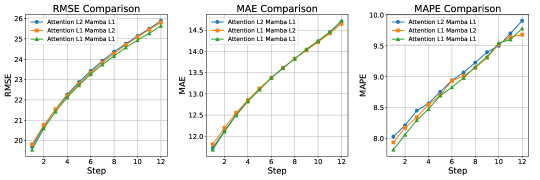
Figure 2: This figure presents a side-by-side comparison of three key performance metrics: Root Mean Square Error (RMSE), Mean Absolute Error (MAE), and Mean Absolute Percentage Error (MAPE), across varying layers of attention and mamba for ST-MambaSync. Each subplot illustrates the variation of a specific metric across 12 time steps, highlighting the models’ performance stability and accuracy in forecasting. Distinct color-coded lines represent different model configurations, ensuring clear differentiation and readability.

In Figure 2, we present an hour-long forecast for PEMS08, visualizing predictions for each 5-minute time step for the metrics RMSE, MAE, and MAPE.The figure presents a comparison of performance metrics for ST-MambaSync: "Attention L2 Mamba L1" and "Attention L1 Mamba L2". The metrics evaluated include Root Mean Square Error (RMSE), Mean Absolute Error (MAE), and Mean Absolute Percentage Error (MAPE) across different prediction steps. In all three metrics, both models exhibit similar trends, with RMSE and MAE increasing gradually with each step, while MAPE shows slight fluctuations. Notably, "Attention L2 Mamba L1" consistently outperforms "Attention L1 Mamba L2" across all metrics and steps, demonstrating its superiority in predicting traffic flow dynamics. The comparison underscores the effectiveness of leveraging both attention and Mamba blocks in enhancing prediction accuracy. Furthermore, it highlights the importance of model architecture in achieving superior performance in traffic forecasting tasks. These findings contribute to the advancement of traffic prediction methodologies, with implications for real-world applications in urban planning and traffic management systems.

7 Conclusion

In summary, this study introduces ST-MambaSync, a novel framework blending an optimized attention layer with a simplified state-space layer. Our experiments show that ST-MambaSync achieves state-of-the-art accuracy in spatial-temporal prediction tasks while minimizing computational costs. By revealing Mamba’s function akin to attention within a residual network structure, we highlight the efficiency of state-space models. This balance between accuracy and efficiency holds promise for various real-world applications, from urban planning to traffic management.

References

- Nagy and Simon (2018) Attila M Nagy and Vilmos Simon. Survey on traffic prediction in smart cities. Pervasive and Mobile Computing, 50:148–163, 2018.
- Smith (1995) Brian Lee Smith. Forecasting freeway traffic flow for intelligent transportation systems application. University of Virginia, 1995.
- Kumar and Vanajakshi (2015) S Vasantha Kumar and Lelitha Vanajakshi. Short-term traffic flow prediction using seasonal arima model with limited input data. European Transport Research Review, 7:1–9, 2015.
- Wu et al. (2004) Chun-Hsin Wu, Jan-Ming Ho, and Der-Tsai Lee. Travel-time prediction with support vector regression. IEEE transactions on intelligent transportation systems, 5(4):276–281, 2004.
- Sayed et al. (2023) Sayed A. Sayed, Yasser Abdel-Hamid, and Hesham Ahmed Hefny. Artificial intelligence-based traffic flow prediction: a comprehensive review. Journal of Electrical Systems and Information Technology, 10(1):13, 2023. ISSN 2314-7172. doi: 10.1186/s43067-023-00081-6. URL https://doi.org/10.1186/s43067-023-00081-6.
- Gu and Dao (2024) Albert Gu and Tri Dao. Mamba: Linear-time sequence modeling with selective state spaces, 2024. URL https://openreview.net/forum?id=AL1fq05o7H.
- Cui et al. (2021) Yue Cui, Jiandong Xie, and Kai Zheng. Historical inertia: A neglected but powerful baseline for long sequence time-series forecasting. In Proceedings of the 30th ACM international conference on information & knowledge management, pages 2965–2969, 2021.
- Wu et al. (2020a) Zonghan Wu, Shirui Pan, Guodong Long, Jing Jiang, Xiaojun Chang, and Chengqi Zhang. Connecting the dots: Multivariate time series forecasting with graph neural networks. In Proceedings of the 26th ACM SIGKDD international conference on knowledge discovery & data mining, pages 753–763, 2020a.
- Li et al. (2018) Yaguang Li, Rose Yu, Cyrus Shahabi, and Yan Liu. Diffusion convolutional recurrent neural network: Data-driven traffic forecasting. In International Conference on Learning Representations, 2018. URL https://openreview.net/forum?id=SJiHXGWAZ.
- Bai et al. (2020) Lei Bai, Lina Yao, Can Li, Xianzhi Wang, and Can Wang. Adaptive graph convolutional recurrent network for traffic forecasting. Advances in neural information processing systems, 33:17804–17815, 2020.
- Yu et al. (2018) Bing Yu, Haoteng Yin, and Zhanxing Zhu. Spatio-temporal graph convolutional networks: A deep learning framework for traffic forecasting. In Proceedings of the Twenty-Seventh International Joint Conference on Artificial Intelligence, IJCAI-18, pages 3634–3640. International Joint Conferences on Artificial Intelligence Organization, 7 2018. doi: 10.24963/ijcai.2018/505. URL https://doi.org/10.24963/ijcai.2018/505.
- Shang et al. (2021) Chao Shang, Jie Chen, and Jinbo Bi. Discrete graph structure learning for forecasting multiple time series. In International Conference on Learning Representations, 2021. URL https://openreview.net/forum?id=WEHSlH5mOk.
- Wu et al. (2020b) Zonghan Wu, Shirui Pan, Guodong Long, Jing Jiang, Xiaojun Chang, and Chengqi Zhang. Connecting the dots: Multivariate time series forecasting with graph neural networks. Proceedings of the 26th ACM SIGKDD International Conference on Knowledge Discovery & Data Mining, 2020b. URL https://api.semanticscholar.org/CorpusID:218869770.
- Zheng et al. (2020) Chuanpan Zheng, Xiaoliang Fan, Cheng Wang, and Jianzhong Qi. Gman: A graph multi-attention network for traffic prediction. Proceedings of the AAAI Conference on Artificial Intelligence, 34(01):1234–1241, Apr. 2020. doi: 10.1609/aaai.v34i01.5477. URL https://ojs.aaai.org/index.php/AAAI/article/view/5477.
- Jiang et al. (2023) Jiawei Jiang, Chengkai Han, Wayne Xin Zhao, and Jingyuan Wang. Pdformer: Propagation delay-aware dynamic long-range transformer for traffic flow prediction. In Brian Williams, Yiling Chen, and Jennifer Neville, editors, Thirty-Seventh AAAI Conference on Artificial Intelligence, AAAI 2023, Thirty-Fifth Conference on Innovative Applications of Artificial Intelligence, IAAI 2023, Thirteenth Symposium on Educational Advances in Artificial Intelligence, EAAI 2023, Washington, DC, USA, February 7-14, 2023, pages 4365–4373. AAAI Press, 2023. doi: 10.1609/AAAI.V37I4.25556. URL https://doi.org/10.1609/aaai.v37i4.25556.
- Liu et al. (2023) Hangchen Liu, Zheng Dong, Renhe Jiang, Jiewen Deng, Jinliang Deng, Quanjun Chen, and Xuan Song. Spatio-temporal adaptive embedding makes vanilla transformer sota for traffic forecasting. In Proceedings of the 32nd ACM International Conference on Information and Knowledge Management, CIKM ’23, page 4125–4129, New York, NY, USA, 2023. Association for Computing Machinery. ISBN 9798400701245. doi: 10.1145/3583780.3615160. URL https://doi.org/10.1145/3583780.3615160.
- Deng et al. (2021) Jinliang Deng, Xiusi Chen, Renhe Jiang, Xuan Song, and Ivor W. Tsang. St-norm: Spatial and temporal normalization for multi-variate time series forecasting. In Proceedings of the 27th ACM SIGKDD Conference on Knowledge Discovery & Data Mining, KDD ’21, page 269–278, New York, NY, USA, 2021. Association for Computing Machinery. ISBN 9781450383325. doi: 10.1145/3447548.3467330. URL https://doi.org/10.1145/3447548.3467330.
- Shao et al. (2022) Zezhi Shao, Zhao Zhang, Fei Wang, Wei Wei, and Yongjun Xu. Spatial-temporal identity: A simple yet effective baseline for multivariate time series forecasting. In Proceedings of the 31st ACM International Conference on Information & Knowledge Management, CIKM ’22, page 4454–4458, New York, NY, USA, 2022. Association for Computing Machinery. ISBN 9781450392365. doi: 10.1145/3511808.3557702. URL https://doi.org/10.1145/3511808.3557702.
- Shao et al. (2024) Zhiqi Shao, Michael G. H. Bell, Ze Wang, D. Glenn Geers, Haoning Xi, and Junbin Gao. St-ssms: Spatial-temporal selective state of space model for traffic forecasting, 2024.