Quantum metrology in a driven-dissipation down-conversion system beyond the parametric approximation
Abstract
We investigate quantum metrology in a degenerate down-conversion system composed of a pump mode and two degenerate signal modes. In the conventional parametric approximation, the pump mode is assumed to be constant, not a quantum operator. We obtain the measurement precision of the coupling strength between the pump mode and two degenerate signal modes beyond the parametric approximation. Without a dissipation, the super-Heisenberg limit can be obtained when the initial state is the direct product of classical state and quantum state. This does not require the use of entanglement resources which are not easy to prepare. When the pump mode suffers from a single-photon dissipation, the measurement uncertainty of the coupling strength is close to 0 as the coupling strength approaches 0 with a coherent driving. The direct photon detection is proved to be the optimal measurement. This result has not been changed when the signal modes suffer from the two-photon dissipation. When the signal modes also suffer from the single-mode dissipation, the information of the coupling strength can still be obtained in the steady state. In addition, the measurement uncertainty of the coupling strength can also be close to 0 and become independent of noise temperature as the critical point between the normal and superradiance phase approaches. Finally, we show that a driven-dissipation down-conversion system can be used as a precise quantum sensor to measure the driving strength.
I Introduction
Quantum metrology mainly studies how to use quantum resources to improve the precision of parameter measurement over classical resourceslab1 ; lab2 ; lab3 ; lab4 ; lab5 ; lab6 . The quantum resources, such as superposition and entanglement, offer a possibility to make the measurement precision with linear generator scale as with being the total average number of photons, which is the Heisenberg scalinglab7 . However, classical resources only get the scaling at most, which is the standard quantum limitlab4 . By using nonlinear generator or time-dependent evolutions, the super-Heisenberg limit can be obtainedlab7a1 ; lab7a2 ; lab7a3 ; lab7a4 .
The parametric down-conversion is relatively easy to become a source of entangled photon pairslab8 , which plays an important role in quantum information processing. Moreover, the parametric down-conversion can be used to build optical parametric amplifiers, which is the main difference between nonlinear SU(1,1)-interferometers and the linear SU(2)-interferometers. SU(1,1)-interferometers offer a platform for multi-photon absorptionlab9 ; lab10 ; lab11 ; lab12 , phase measurementlab12a , loss-tolerant quantum metrologylab13 ; lab14 , Wigner function tomographylab15 , and quantum state engineeringlab16 ; lab17 .
Most of the previous work has used the parametric approximationlab18 to deal with the down-conversion process, where the number of pump mode is assumed to be constant. This parametric approximation can give an exact description of the system dynamics at short times, but the resulting state will become invalid as the number of pump photons decreases with time. Recently, K. Chinni and N. Quesadalab19 used the cumulant expansion method, perturbation theory, and the full numerical simulation of systems to deal with the closed down-conversion process beyond the parametric approximation. However, quantum metrology beyond parametric approximation in parametric down-conversion systems, especially in the case of driven-dissipation, has not been studied at present.
This inspires us to try to fill the gap. In this article, we investigate quantum metrology in a degenerate down-conversion system composed of a pump mode and two degenerate signal modes. In the closed system, we analytically obtain the quantum Fisher information of the nonlinear coupling strength between the pump mode and the signal modes. It shows that the super-Heisenberg limit can be obtained without using preparative entangled or squeezed states, just the signal modes in the Fock state. The reason for obtaining the super-Heisenberg limit is the nonlinear generator of . When the pump mode suffers from a single-photon dissipation, the measurement uncertainty of the coupling strength is close to 0 as the coupling strength approaches 0 due to a continuous coherent driving. By comparing with the results achieved by the quantum Fisher information, the direct photon detection is proved to be the optimal measurement. This result has not been changed when the signal modes suffer from the two-photon dissipation. When the signal modes also suffer from the single-mode dissipation, the information of very weak coupling strength can still be obtained with a finite precision under steady state. Finally, the measurement uncertainty of the coupling strength can also be close to 0 and become independent of the temperature of the noise as the critical point between the normal and superradiance phase approaches.
This article is organized as follows. In section II, quantum metrology in a closed degenerate down-conversion system is studied. In section III, quantum metrology in a driven-dissipation degenerate down-conversion system is studied in different cases. Quantum sensor of the driving strength is explored in section IV. Finally, we make a simple conclusion and outlook in section V.
II degenerate down-conversion system
We consider that the Hamiltonian describing the degenerate down-conversion process on resonance ()is given by
| (1) |
where is the annihilation (creation) bosonic operator for the pump mode with the frequency , and is the annihilation (creation) operator for the signal mode with the frequency . The operators and satisfy the canonic commutation relation, i.e., with . Without loss of generality, the coupling strength is chosen to be the real quantity and through this article.
In the interaction picture, the Hamiltonian is rewritten as
| (2) |
For the pure state , the quantum Fisher information for the parameter can be calculated bylab20 ; lab21
| (3) |
where and .
When the initial state is a semi-classical state (direct product of classical state and quantum state) with the coherent state and the Fock state , we can obtain that . Given by the fixed total number of photons, , the optimal estimation precision is obtained with for ,
| (4) |
When the initial state is a complete quantum state (direct product of quantum state and quantum state) with , . The optimal estimation precision can be achieved when for ,
| (5) |
Obviously, the optimal measurement precision is the same for the complete quantum state and the semi-classical state, i.e., .
For the complete classical initial state , the according quantum Fisher information is . Given by the constraint condition , the maximal quantum Fisher information is achieved when . It shows that the complete classical state can not perform better than the complete quantum state and the semi-classical state. In the down-conversion system, the super-Heisenberg limit can be obtained only if the initial state of the signal mode is quantum state, where entangled or squeezed states that are difficult to prepare are not required. The reason for obtaining the super-Heisenberg limit is due to the fact that the generator is nonlinear.
III driven-dissipation system
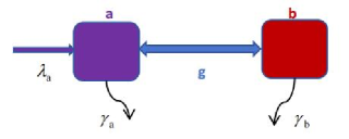
In this section, we consider that the degenerate down-conversion system suffers from an inevitably dissipative environment, as shown in Fig. 1. In order to resist the dissipation, we consider that there is an extra coherent driving . The evolution of the density matrix of the driven-dissipation system is described by the master equation
| (6) |
where the superoperator with . The corresponding quantum Langevin-Heisenberg equation of a operator is derived bylab22 ; lab23 ; lab24
| (7) |
Utilizing the above equation, let , we can obtain the evolution dynamics
| (8) | ||||
| (9) |
where the expected values of the noise operators are , and with .
III.1 In the case of
When the decay rate is much lager than (), the pump mode can be adiabatically eliminated. Let , we obtain
| (10) |
Substituting the above equation into Eq. (7), we obtain that
| (11) |
By combining Eq. (6) with Eq. (7), we can get the reduced master equation of the signal mode, which is described as
| (12) |
where and .
The steady state can be analytically derived by a complex P-representation solutionlab25 or Keldysh-Heisenberg equationlab26 . The general form can be expressed as
| (13) |
where the normalization factor , and the function , in which , , and . The Gauss hypergeometric function is described by
| (14) |
where the function and denotes the Gamma function.
III.1.1 In the case of
When the decay rate , the expected value in Eq. (13) can be simplified as
| (15) |
With the specific measurement operator , the measurement uncertainty of the parameter can be calculated by the error propagation formula
| (16) |
For the direct photon detection with , the uncertainty of the parameter is derived by the above equation
| (17) |
For the homodyne detection with , the uncertainty of the parameter is given by
| (18) |
When , i.e., the Homodyne detection , the above measurement uncertainty is optimized,
| (19) |
Comparing Eq. (17) with Eq. (19), we find that the direct photon detection performs better than the homodyne detection. All results show that the uncertainty is close to 0 as the parameter . It is due to the fact that the subsystem of the signal mode can not arrive at the steady state when . At this point, the total number of photons tends to infinity as goes to 0, i.e., . It is due to the fact that the infinite encoding time makes the measurement uncertainty become 0. Using , Eq. (17) can be reexpressed as
| (20) |
It shows that the super-Heisenberg scaling of the single photon dissipation of the pump mode can be obtained by local measurement of the signal mode without considering the time consumption.
III.1.2 Extra two-photon dissipation
Then, we consider that the signal mode suffers from an extra two-photon dissipation with dissipation rate . The total evolution dynamics of the signal mode is described by
| (21) |
When the decay rate , the expectated values can be simplified as
| (22) |
Using the direct photon detection, the measurement uncertainty of the parameter is given by
| (23) |
For the Gaussian state, the quantum Fisher information is derived bylab27 ; lab28
| (24) |
where with quadrature operators defined as: , and . And the entries of the covariance matrix are defined as . is given by .
Based on the expected values in Eq. (22), we obtain that
Then, we derive that . As a result, the quantum Fisher information can be obtained
| (25) | |||
| (26) |
According to the quantum Cramér-rao boundlab29 ; lab30 ; lab31 , the measurement uncertainty is given by
| (27) |
Comparing with the result obtained by the direct detection in Eq. (23), it obviously shows that the direct detection is the optimal measurement, which can obtain the optimal measurement precision.
The above result shows that the measurement uncertainty is also close to 0 as goes to 0. In order to explain this, we calculate the characteristic time for the system to reach steady state. Let , keeping only the linear terms, the evolution of is reduced to
| (28) |
According to the above equation, the characteristic time to steady state is given by
| (29) |
This result shows that the characteristic time is divergent at . The two-photon dissipation does not allow the signal mode to reach the steady state. The intuitive explanation is that there are subspaces that are not subject to two-photon dissipation.
III.1.3 Three-level approximation in the case of
Expanding on the Fock basis , Eq. (21) can be rewritten as
| (30) |
We consider a weak coupling , . The effective two-photon driving is weak. Therefore, the subsystem is at a low energy level. We consider the three-level subsystem with . Keeping only the lowest three energy levels, Eq. (30) is reduced to the following formulas
| (31) | ||||
| (32) | ||||
| (33) | ||||
| (34) |
where . Let the left terms of the above equations be 0, the steady-state solutions are given by
| (35) | |||
| (36) | |||
| (37) | |||
| (38) | |||
| (39) |
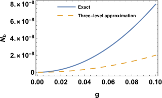
By calculating the expected value from the three-level approximation method and the master equation in Eq. (12), we can find that the three-level approximation is more and more accurate as the coupling strength decreases, as shown in Fig. 2.
With the direct photon detection, the measurement uncertainty of the coupling strength is given by
| (40) |
With the homodyne detection, the measurement uncertainty is given by
| (41) |
When the density matrix is expressed in diagonal form with the eigenstate , , the quantum Fisher information can be calculated by
| (42) |
After a simple calculation according to the above equation, the quantum Fisher information is given by
| (43) |
According to the quantum Cramér-rao bound, the measurement uncertainty is given by
| (44) |
Comparing the above equation with Eq. (40) and Eq. (41), it shows that the direct homodyne detection is close to the optimal measurement.
When there are single photon dissipation, i.e., , the characteristic time to steady state is given by when the coupling strength . In the steady state, the total photon number is given by . When , the total photon number . This result is interesting. Although the total photon number in the steady state is close to 0 and the interaction time is finite, the measurement uncertainty of the coupling strength is not infinite. In other words, when the signal mode suffers from the single-photon and two-photon dissipation, the information of the weak coupling strength can still be obtained in the steady state.
III.2 The adiabatic elimination condition is not satisfied
In this subsection, we consider that the adiabatic elimination condition is not satisfied.
Let and , the equations of motion for the steady-state mean values of the operators are derived as
| (47) | ||||
| (48) |
where we use a mean-field like approximation and . We set that and , where , , and are real numbers. The above equations can be rewritten as
| (49) | ||||
| (50) | ||||
| (51) | ||||
| (52) |
By solving the above equations, we obtain
| (53) | ||||
| (54) |
When , the solution (2) does not exist due to the fact that can not be a complex number.
By using that and , we can obtain the linearized quantum Langevin equations by keeping the terms up to the first order of quantum fluctuation:
| (55) |
where the evolution matrix is described as
and the quantum noise operators are .
When , the steady-state solution (, ) ensures that the system is stable. It is due to the fact that all eigenvalues of the evolution matrix have negative real parts.
When , the solution (, ) makes the system unstable. In this case, (, ) can make the system stable. When , we achieve that . It recovers the previous result as shown in Eq. (15).
Generally, it is defined as the normal phase when; and it is defined as the superradiance phase whenlab32 . As the driving strength increases, the system changes from the normal phase to the superradiant phase. The critical point of the phase transition occurs when the driving strength is equal to the critical driving strength .
In the normal phase, we can obtain the analytical solution. Supposing that the system has reached the steady state after a long-time evolution, the solution of the quantum fluctuation operator is
| (56) |
Using the correlation functions of the noise operator , we can obtain the expected values
| (57) | ||||
| (58) | ||||
| (59) |
Using the decoupling relation as shown in ref.lab33 , we obtain the expected value
| (60) |
With the direct photon detection , the measurement uncertainty of is given by
| (61) | ||||
| (62) |
We can find that the measurement uncertainty is close to 0 as the phase transition point approaches, i.e., . As a cost, the time resources used will also tend to be infinite.
III.2.1 Thermal noise with temperature
When the system is subjected to a dissipative environment with a non-zero temperature , the correlated values of the noises of the subsystem are rewritten as
| (63) | ||||
| (64) | ||||
| (65) |
where the average thermal photon number . With the direct photon detection , the measurement uncertainty of is given by
| (66) | ||||
| (67) |
From the above equation, we can obviously see that the measurement uncertainty is also close to 0 as the phase transition point approaches. Near the critical point of the phase transition, (i.e. ), we get a temperature-independent result
| (68) |
It shows that the influence of the temperature of the noise bath on the measurement precision of the coupling parameters tends to 0 near the phase transition point. That is, it is robust to the thermal fluctuations from the dissipative environment.
IV Quantum sensor of the driving strength
In addition to measuring the coupling strength , it can also be used to measure the driving strength . By the similar calculation, in the case of , the measurement precision of is
| (69) |
This result shows that the measurement uncertainty of the driving strength decreases with the decrease of . It means that the dissipative degenerate down-conversion system can be a sophisticated quantum sensor about the weak driving strength when the signal mode does not suffer from the single-photon dissipation. With photon number of the signal mode , the measurement precision of is rewritten as
| (70) |
This means that for only the quantum limit is obtained, and nothing like can obtain the super-Heisenberg limit in Eq. (15). It is due to the fact that the generator of is nonlinear and the generator of is linear. Moreover, we find that the measurement precision of can be enhanced by reducing the coupling strength without the extra two-photon dissipation. However, when , the measurement precision of will decrease as decreases. For , we can achieve the optimal precision of
| (71) |
V Conclusion
We have investigated the quantum metrology in the degenerate down-conversion system. Due to the nonlinear generator of the coupling strength, in the closed system the super-Heisenberg limit can be obtained with the semi-classical initial state. And the measurement precision increases with the evolution time, which gives an intuitive explanation of the results obtained in the dissipation case.
When , we obtain the analytical result by adiabatically eliminating the pump mode. In the case of , the direct photon detection is proved to the optimal measurement. The result shows that the measurement uncertainty is close to 0 as . As a trade-off, the time to steady state also tends to infinity as . Unexpectedly, the above result can not be influenced when the signal mode suffers from two-photon dissipation. The intuitive explanation is that there are subspaces that are not subject to two-photon dissipation. In the case of , an interesting result shows that although the total photon number in the steady state is close to 0 and the interaction time is finite, the measurement uncertainty of the coupling is not infinite. It means that the information of the coupling strength can still be obtained in the steady state no matter how small is.
When the adiabatic elimination condition is not satisfied, there is a critical phase transition point between the normal phase and superradiance phase. We can find that the measurement uncertainty is close to 0 as the phase transition point approaches. As before, it takes an infinite amount of encoding time to get that . And we show that the influence of the temperature of the noise bath on the measurement precision of the coupling parameters tends to 0 near the phase transition point.
Finally, the degenerate down-conversion system can be used as a quantum sensor to measure the coherent driving strength. We show that the measurement uncertainty of the driving strength decreases with the decrease of the driving strength. Only the quantum limit is obtained for , which is due to the fact that the generator of is nonlinear and the generator of is linear. This inspires us to discuss how to convert linear generators into nonlinear generators for improving the measurement precision. Moreover, we find that the measurement precision of can be enhanced by reducing the coupling strength without the extra two-photon dissipation. However, when , the measurement precision of will decrease as decreases.
It is worth further exploring the problems related to multi-photon absorption and multi-parameter simultaneous measurement in the down-conversion system. In experiment, the down-conversion system can be observed typically in uniaxial and noncentrosymmetric medialab34 , a linear trapped three-ion crystallab35 , and a lithium niobate crystallab36 .
Acknowledgements.-This research was supported by the National Natural Science Foundation of China (Grant No. 12365001 and No. 62001134), and Guangxi Natural Science Foundation ( Grant No. 2020GXNSFAA159047).
References
- (1)
- (2) S. Pirandola, B. R. Bardhan, T. Gehring, C. Weedbrook, and S. Lloyd, Advances in photonic quantum sensing, Nat. Photonics 12,724-733 (2018).
- (3) C. L. Degen, F. Reinhard, and P. Cappellaro, Quantum sensing, Rev. Mod. Phys. 89, 035002 (2017).
- (4) V. Giovannetti, S. Lloyd, and L. Maccone, Quantum metrology, Phys. Rev. Lett. 96, 010401 (2006).
- (5) V. Giovanetti, S. Lloyd, L. Maccone Quantum-enhanced measurements: beating the standard quantum limit. Science 306, 1330 (2004).
- (6) D. Xie, and A. Wang, Quantum metrology in correlated environments, Phys. Lett. A 378, 2079 (2014).
- (7) C. W. Helstrom, Quantum Detection and Estimation Theory, Academic, New York, 1976.
- (8) J. Taylor, P. Cappellaro, L. Childress, L. Jiang, D. Budker, P. R. Hemmer, A. Yacoby, R. Walsworth, and M. D. Lukin, High-sensitivity diamond magnetometer with nanoscale resolution, Nat. Phys. 4: 810 (2008).
- (9) C. Napoli, S. Piano, R. Leach, G. Adesso, and T. Tufarelli, Towards superresolution surface metrology: Quantum estimation of angular and axial separations. Phys. Rev. Lett. 122, 140505 (2019).
- (10) Z. Hou, Y. Jin, H. Chen, J. Tang, C. Huang, H. Yuan, G. Xiang, C. Li, and G. Guo, Super-Heisenberg and Heisenberg scalings achieved simultaneously in the estimation of a rotating field. Phys Rev Lett 126, 070503 (2021).
- (11) X. He, R. Yousefjani, and A. Bayat, Stark localization as a resource for weak-field sensing with super-Heisenberg precision, Phys. Rev. Lett. 131, 010801(2023)
- (12) J. Yang, S. Pang, A. d. Campo, A. N. Jordan, Super-Heisenberg scaling in Hamiltonian parameter estimation in the long-range Kitaev chain, Phys. Rev. Research 4, 013133(2022).
- (13) M. H. Rubin, D. N. Klyshko, Y. H. Shih, and A. V. Sergienko, Theory of two-photon entanglement in type-II optical parametric down-conversion, Phys. Rev. A 50, 5122 (1994).
- (14) C. Sanchez Muñoz, G. Frascella, and F. Schlawin, Quantum metrology of two-photon absorption, Phys. Rev. Research 3, 033250 (2021).
- (15) S. Panahiyan, C. S. Muñoz, M. V. Chekhova, and F. Schlawin, Two-photon absorption measurements in the presence of single-photon losses, Phys. Rev. A 106, 043706 (2022).
- (16) C. Drago and J. E. Sipe, Aspects of two-photon absorption of squeezed light: The continuous-wave limit, Phys. Rev. A 106, 023115 (2022).
- (17) S. Panahiyan, C. S. Muñoz, M. V. Chekhova, and F. Schlawin, Nonlinear Interferometry for Quantum-Enhanced Measurements of Multiphoton Absorption, Phys. Rev. Lett. 130, 203604 (2023).
- (18) M. Manceau, G. Leuchs, F. Khalili, and M. Chekhova, Detection loss tolerant supersensitive phase measurement with an su(1,1) interferometer, Phys. Rev. Lett. 119, 223604 (2017).
- (19) Y. Liu, J. Li, L. Cui, N. Huo, S. M. Assad, X. Li, and Z. Y. Ou, Loss-tolerant quantum dense metrology with su(1,1) interferometer, Opt. Express 26, 27705 (2018).
- (20) W. Du, J. Kong, G. Bao, P. Yang, J. Jia, S. Ming, C.-H. Yuan, J. F. Chen, Z. Y. Ou, M. W. Mitchell, and W. Zhang, Su(2)-in su(1,1) nested interferometer for high sensitivity, loss-tolerant quantum metrology, Phys. Rev. Lett. 128, 033601 (2022).
- (21) M.Kalash, and M. V. Chekhova, Wigner function tomography via optical parametric amplification, Opica 10, 1142 (2023).
- (22) S. Lemieux, M. Manceau, P. R. Sharapova, O. V. Tikhonova, R. W. Boyd, G. Leuchs, and M. V. Chekhova, Engineering the frequency spectrum of bright squeezed vacuum via group velocity dispersion in an su(1,1) interferometer, Phys. Rev. Lett. 117, 183601 (2016).
- (23) J. Su, L. Cui, J. Li, Y. Liu, X. Li, and Z. Y. Ou, Versatile and precise quantum state engineering by using nonlinear interferometers, Opt. Express 27, 20479 (2019).
- (24) P. D. Drummond and M. Hillery, The quantum theory of nonlinear optics (Cambridge University Press, 2014).
- (25) K. Chinni, and N. Quesad, Beyond the parametric approximation: pump depletion, entanglement and squeezing in macroscopic down-conversion, arXiv:2312.09239 (2023).
- (26) C. W. Helstrom, Quantum Detection and Estimation Theory (New York: Academic) 1976.
- (27) A. S. Holevo, Probabilistic and Statistical Aspects of Quantum Theory (Amsterdam: North Holland) 1982.
- (28) C. Gardiner, and P. Zoller, Qauntum Noise: A Handbook of Markovian and Non-Markovian Quantum Stochastic Methods with Applications to Quantum Optics, vol. 56 (Springer, Berlin, 2004).
- (29) M. Reitz, C. Sommer, and C. Genes, Langevin approach to quantum optics with molecules, Phys. Rev. Lett. 122, 203602 (2019).
- (30) D. Xie, C. Xu, and A. M. Wang, Quantum thermometry with a dissipative quantum Rabi system, Eur. Phys. J. Plus 137:1323 (2022).
- (31) N. Bartolo, F. Minganti, W. Casteels, and C. Ciuti, Exact steady state of a Kerr resonator with one- and two-photon driving and dissipation: Controllable wigner function multimodality and dissipative phase transitions. Phys. Rev. A 94, 033841 (2016).
- (32) Y. Zhang, and G. Chen, Method for driven-dissipative problems: Keldysh- Heisenberg equations, Phys. Rev. A 102, 062205 (2020).
- (33) A. Monras, Phase space formalism for quantum estimation of Gaussian states, arXiv:1303.3682 (2013).
- (34) L. Garbe, M. Bina, A. Keller, M. G. A. Paris, S. Felicetti, Critical quantum metrology with a finite-component quantum phase transition. Phys. Rev. Lett. 124, 120504 (2020).
- (35) H. Cramér, Mathematical Methods of Statistics (Princeton University, Princeton, 1946).
- (36) C.R. Rao, Linear Statistical Inference and Its Applications (Wiley, NewYork, 1973).
- (37) S.L. Braunstein, C.M. Caves, Statistical distance and the geometry of quantum states. Phys. Rev. Lett. 72, 3439 (1994).
- (38) A. Baksic and C. Ciuti, Controlling Discrete and Continuous Symmetries in Superradiant Phase Transitions with Circuit QED Systems, Phys. Rev. Lett. 112, 173601 (2014).
- (39) J. Naikoo, K. Thapliyal, A. Pathak, S. Banerjee, Probing nonclassicality in an optically driven cavity with two atomic ensembles. Phys. Rev. A 97,063840 (2018).
- (40) R. W. Boyd, Nonlinear Optics (Academic Press, 2020).
- (41) J. Flórez, J. S. Lundeen, and M. V. Chekhova, Pump depletion in parametric down-conversion with low pump energies, Optics Letters 45, 4264 (2020).
- (42) S. Ding, G. Maslennikov, R. Hablützel, and D. Matsukevich, Quantum simulation with a trilinear hamiltonian, Physical Review Letters 121, 130502 (2018).