Department of Statistics
Raleigh, North Carolina 27695, U.S.A.
11email: {rgmarti3, jwilli27}@ncsu.edu
Large-sample theory for inferential models: a possibilistic Bernstein–von Mises theorem
Abstract
The inferential model (IM) framework offers alternatives to the familiar probabilistic (e.g., Bayesian and fiducial) uncertainty quantification in statistical inference. Allowing this uncertainty quantification to be imprecise makes it possible to achieve exact validity and reliability. But is imprecision and exact validity compatible with attainment of the classical notions of statistical efficiency? The present paper offers an affirmative answer to this question via a new possibilistic Bernstein–von Mises theorem that parallels a fundamental result in Bayesian inference. Among other things, our result demonstrates that the IM solution is asymptotically efficient in the sense that its asymptotic credal set is the smallest that contains the Gaussian distribution whose variance agrees with the Cramér–Rao lower bound.
Keywords:
Asymptotics; Bayesian; belief; fiducial; relative likelihood1 Introduction
Efron, (2013) writes that “the most important unresolved problem in statistical inference is the use of Bayes theorem in the absence of prior information.” Numerous attempts have been made, including Bayesian inference with default priors, from Laplace’s flat priors to the refinements by Jeffreys, (1946) and Berger et al., (2009), fiducial inference in Fisher’s original sense (Fisher, 1935; Zabell, 1992) and its generalizations (Fraser, 1968; Hannig et al., 2016; Dempster, 1967, 2008), and the various imprecise-probabilistic proposals (e.g., Berger, 1984; Walley, 1991; Dubois, 2006; Augustin et al., 2014). One thing that many of these solutions offer is a large-sample result which states, roughly, that the associated credible sets achieve the nominal frequentist coverage probability when the sample size, , is large. Statisticians insist on methods that are demonstrably reliable in the sense of tending to report “correct inferences” across repeated uses, so results like this are high-value. The résultat extraordinaire along these lines is the Bernstein–von Mises theorem which states the following: under certain conditions, the Bayesian or fiducial posterior distribution is approximately Gaussian, centered at the maximum likelihood estimator, and is efficient in the sense that its variance equals the Cramér–Rao lower bound; here “approximately” is in the sense that the total variation distance between the two distributions is vanishing in probability as . For details, see van der Vaart, (1998, Ch. 10), Ghosh et al., (2006, Ch. 4), or Hannig et al., (2016).
Still, none of the Bayesian- or fiducial-like solutions mentioned above have proved to be fully satisfactory. One possible explanation is that large-sample confidence sets don’t tell the whole story. Indeed, the false confidence theorem (Balch et al., 2019; Martin, 2019) implies that, at every , there exists false hypotheses about the unknown to which the (Bayesian or fiducial) posterior will tend to assign relatively high probability—that is, the posterior probability assignments have an inherent unreliability. To avoid this pitfall, it’s necessary that the Bayesian or fiducial precise probability be replaced by a data-dependent imprecise probability. The inferential model (IM) framework, including the original developments in Martin and Liu, (2013, 2015) and the more recent generalizations in Martin, (2021); Martin, 2022a ; Martin, 2022b , does just this. Moreover, the IM is provably valid in a sense that implies it’s safe from false confidence and, e.g., it provides exact finite-sample confidence sets. While the IM solution’s efficiency compared to existing solutions—Bayesian, frequentist, or otherwise—has been determined empirically in specific applications, a general theoretical statement concerning its efficiency is lacking. In this paper, for the class of IMs in Martin, (2015, 2018); Martin, 2022b , we establish a possibilistic version of the Bernstein–von Mises theorem that parallels those mentioned above. Among other things, this result confirms our conjecture that, despite the genuine imprecision in the IM’s output needed to ensure exact validity, there’s no loss of efficiency asymptotically.
2 Background
2.1 Possibility theory
Possibility theory is among the simplest imprecise probability theories, corresponding to consonant belief structures (e.g., Shafer, 1976, Ch. 10). Other key references include Zadeh, (1978), Dubois and Prade, (1988), and Dubois, (2006). The simplicity of possibilistic uncertainty quantification comes from its parallels to precise probability theory. A necessity–possibility measure pair that’s intended to quantify uncertainty about an uncertain in is determined by a possibility contour , with , via the rules
So, where ordinary probability is determined by integrating a density function, possibility is determined by optimizing a contour. The above values are often interpreted subjectively as (coherent) upper and lower probabilities associated with the proposition “” or as Shaferian degrees of belief.
One way to elicit a possibility measure, specifically relevant to us here, is via the probability-to-possibility transform (e.g., Dubois et al., 2004; Hose, 2022). If is a probability density function, which determines a random variable , then the probability-to-possibility transform defines as
This defines the “best approximation” of by a possibility measure in the sense that its corresponding credal set is the smallest one that contains . If is the (multivariate) standard normal density on , the probability-to-possibility transform has contour defined as as shown in Figure 1(a); the corresponding Gaussian possibility measure defined via optimization is denoted by .
2.2 Inferential models
The original IM constructions (e.g., Martin and Liu, 2013, 2015) were formulated in terms of (nested) random sets and, hence, the connection to possibility theory was indirect. A more recent IM construction introduced in Martin, 2022b —see, also, Martin, (2015, 2018)—directly defines the IM’s possibility contour using a version of the probability-to-possibility transform. An advantage of this alternative perspective and construction is that it avoids the ambiguity in specifying both a data-generating equation and a so-called “predictive random set.”
The statistical model assumes that consists of iid samples from a distribution depending on an unknown/uncertain to be inferred. The model and observed data together determine a likelihood function and a corresponding relative likelihood function
The relative likelihood itself defines a data-dependent possibility contour that has been widely studied (e.g., Shafer, 1982; Wasserman, 1990; Denœux, 2006, 2014). Most appealing about the likelihood-based possibility contour is its shape: peak at the maximum likelihood estimator and consistent with Fisher’s suggested likelihood-based preference order on the parameter space. But it lacks a standard scale, i.e., what constitutes a “small” relative likelihood depends on aspects of the individual application. A (literally) uniform scale of interpretation across applications can easily be obtained via what Martin, 2022a calls “validification,” which is a sort of possibilistic transform. In particular, for observed data , the possibilistic IM’s contour is
| (1) |
and the corresponding possibility measure is
Critical to the IM developments is the so-called validity property which can be succinctly described by the following expression:
| (2) |
This is precisely the universal scaling that the relative likelihood itself is missing, i.e., “” has the same inferential meaning/force in every application. It also implies that the IM is safe from false confidence. Finally, it has some important and familiar statistical consequences:
-
•
a test that rejects the hypothesis “” when will control the frequentist Type I error rate at level , and
-
•
the set is a % frequentist confidence set in the sense that its coverage probability is at least .
Given that the IM is inherently imprecise and offers finite-sample guarantees, the reader might think that this comes with an associated loss of efficiency compared to those methods whose justification relies on asymptotic considerations. The result in the next section aims to debunk this myth.
3 A possibilistic Bernstein–von Mises theorem
3.1 Preview
To build some intuition, consider a simple exactly Gaussian model where is an iid sample from , where the mean is unknown but is known. The maximum likelihood estimator is , the sample mean, and it is not difficult to show that the IM’s possibility contour is
where is the Gaussian possibility contour in Section 2.1. Alternatively, if we switch to a local parametrization of , i.e., , then
For a generic , the corresponding possibility measure is
where is the Gaussian possibility measure from Section 2.1 and, for constants and , the set is defined as .
Once we step away from an exact Gaussian model, there is no longer an exact correspondence between the possibilistic IM’s solution and the Gaussian possibility measure. It’s a similar story in the Bayesian and (generalized) fiducial case. But the probabilistic Bernstein–von Mises theorem implies that, under certain conditions, as , the suitably centered and scaled Bayesian posterior distribution will be approximately Gaussian. Our main result shows that the same holds true for the possibilistic IM solution: under certain regularity conditions, a suitably centered and scaled version of the IM’s possibility measure will converge in a strong sense to the Gaussian possibility measure.
3.2 Main result
The regularity conditions stated below are exactly those assumed in textbook treatments of the asymptotic normality of maximum likelihood estimators—in particular, Schervish, (1995, Theorem 7.63).
Regularity Conditions 1
The probability measures , indexed by , have density functions with respect to a fixed dominating measure. Recall that denotes the special “true” parameter value.
-
1.
The support of doesn’t depend on .
-
2.
is twice continuously differentiable for almost all .
-
3.
Differentiation can be passed under the integral sign.
-
4.
The second derivative of is Lipschitz continuous in a neighborhood of with Lipschitz constant that has finite -expectation.
Under the above regularity conditions, we establish a possibilistic Bernstein–von Mises theorem for the IM solution presented in Section 2.2. That is, a centered and scaled version of the IM’s possibility contour, namely,
| (3) |
where denotes the observed Fisher information matrix, can be well approximated by the Gaussian possibility contour.
Theorem 3.1
Let consist of iid observations from , where is the posited model and is in the interior of . If the above regularity conditions hold at , and the maximum likelihood estimator is consistent, then the possibilistic IM’s solution satisfies
| (4) |
where is an arbitrary compact set, is as in (3), and is the Gaussian contour. This, in turn, implies that
for all compact with .
The proof of Theorem 3.1 is lengthy and will be presented elsewhere. While it follows immediately from Wilks, (1938) that in distribution under , for , getting the required in-probability convergence uniformly over parameter values requires significant care.
Why does in (4) exclude the origin? It’s because there’s a sort of singularity, i.e., is identically 1, no sampling variability! Since we know that exactly, it suffices to focus on values away from the origin (and from infinity). Similarly, open subsets that contain will also eventually contain and, consequently, with high probability when is large. Therefore, it suffices to focus on compact that exclude .
The take-away message is that there’s now a mathematically rigorous sense in which this possibilistic IM—despite its imprecision and exact validity—is also statistically efficient. This also shows that the connection between the possibilistic IMs and Bayes/fiducial solutions highlighted in Martin, (2023) for a special class of models holds much more broadly, asymptotically. Finally, other asymptotically equivalent scaling schemes can be employed in (3). For example, replacing with leads to a limiting Gaussian possibility with underlying covariance matrix matching the Cramér–Rao lower bound.
4 Numerical illustrations
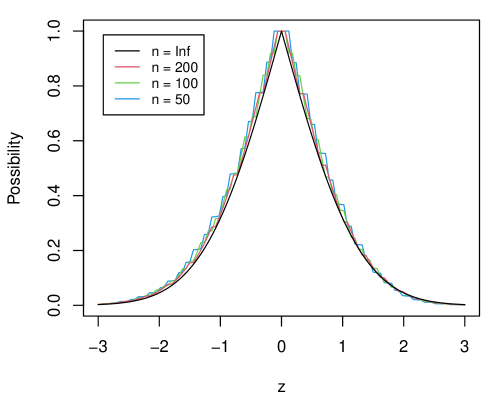
Example 1
iid Bernoulli. Figure 1(a) shows the exact centered and scaled possibilistic IM contour for based on iid Bernoulli data at three different sample sizes, along with the limiting standard Gaussian possibility contour.
Example 2
Logistic regression. Consider the data in Table 8.4 of Ghosh et al., (2006, p. 252) on the relationship between exposure to chloracetic acid and the death of mice. A total of mice are exposed, ten at each of the twelve dose levels, and a binary death indicator is measured. A simple logistic regression model is fit and Figure 1(b) shows the exact IM possibility contour (red)—which requires expensive but still noisy Monte Carlo evaluations—along with the simple, analytically tractable Gaussian approximation (black).

5 Conclusion
This paper establishes a possibilistic Bernstein–von Mises theorem for the possibilistic IM solution which, in addition to providing new insights and connections to the more familiar Bayesian and fiducial solutions, leads to theoretically and practically important conclusions concerning the IM’s efficiency. Follow-up work will consider extensions of our present result to cases that involve nuisance parameters and/or partial prior information about the unknowns.
5.0.1 Acknowledgements
RM’s research is supported by the U.S. National Science Foundation, SES–2051225.
5.0.2 \discintname
The authors have no competing interests to declare that are relevant to the content of this article.
References
- Augustin et al., (2014) Augustin, T., Walter, G., and Coolen, F. P. A. (2014). Statistical inference. In Introduction to Imprecise Probabilities, Wiley Ser. Probab. Stat., pages 135–189. Wiley, Chichester.
- Balch et al., (2019) Balch, M. S., Martin, R., and Ferson, S. (2019). Satellite conjunction analysis and the false confidence theorem. Proc. Royal Soc. A, 475(2227):2018.0565.
- Berger, (1984) Berger, J. O. (1984). The robust Bayesian viewpoint. In Robustness of Bayesian Analyses, volume 4 of Stud. Bayesian Econometrics, pages 63–144. North-Holland, Amsterdam. With comments and with a reply by the author.
- Berger et al., (2009) Berger, J. O., Bernardo, J. M., and Sun, D. (2009). The formal definition of reference priors. Ann. Statist., 37(2):905–938.
- Dempster, (1967) Dempster, A. P. (1967). Upper and lower probabilities induced by a multivalued mapping. Ann. Math. Statist., 38:325–339.
- Dempster, (2008) Dempster, A. P. (2008). The Dempster–Shafer calculus for statisticians. Internat. J. Approx. Reason., 48(2):365–377.
- Denœux, (2006) Denœux, T. (2006). Constructing belief functions from sample data using multinomial confidence regions. Internat. J. of Approx. Reason., 42(3):228–252.
- Denœux, (2014) Denœux, T. (2014). Likelihood-based belief function: justification and some extensions to low-quality data. Internat. J. Approx. Reason., 55(7):1535–1547.
- Dubois, (2006) Dubois, D. (2006). Possibility theory and statistical reasoning. Comput. Statist. Data Anal., 51(1):47–69.
- Dubois et al., (2004) Dubois, D., Foulloy, L., Mauris, G., and Prade, H. (2004). Probability-possibility transformations, triangular fuzzy sets, and probabilistic inequalities. Reliab. Comput., 10(4):273–297.
- Dubois and Prade, (1988) Dubois, D. and Prade, H. (1988). Possibility Theory. Plenum Press, New York.
- Efron, (2013) Efron, B. (2013). Discussion: “Confidence distribution, the frequentist distribution estimator of a parameter: a review” [mr3047496]. Int. Stat. Rev., 81(1):41–42.
- Fisher, (1935) Fisher, R. A. (1935). The fiducial argument in statistical inference. Ann. Eugenics, 6:391–398.
- Fraser, (1968) Fraser, D. A. S. (1968). The Structure of Inference. John Wiley & Sons Inc., New York.
- Ghosh et al., (2006) Ghosh, J. K., Delampady, M., and Samanta, T. (2006). An Introduction to Bayesian Analysis. Springer, New York.
- Hannig et al., (2016) Hannig, J., Iyer, H., Lai, R. C. S., and Lee, T. C. M. (2016). Generalized fiducial inference: a review and new results. J. Amer. Statist. Assoc., 111(515):1346–1361.
- Hose, (2022) Hose, D. (2022). Possibilistic Reasoning with Imprecise Probabilities: Statistical Inference and Dynamic Filtering. PhD thesis, University of Stuttgart.
- Jeffreys, (1946) Jeffreys, H. (1946). An invariant form for the prior probability in estimation problems. Proc. Roy. Soc. London Ser. A, 186:453–461.
- Martin, (2015) Martin, R. (2015). Plausibility functions and exact frequentist inference. J. Amer. Statist. Assoc., 110(512):1552–1561.
- Martin, (2018) Martin, R. (2018). On an inferential model construction using generalized associations. J. Statist. Plann. Inference, 195:105–115.
- Martin, (2019) Martin, R. (2019). False confidence, non-additive beliefs, and valid statistical inference. Internat. J. Approx. Reason., 113:39–73.
- Martin, (2021) Martin, R. (2021). An imprecise-probabilistic characterization of frequentist statistical inference. arXiv:2112.10904.
- (23) Martin, R. (2022a). Valid and efficient imprecise-probabilistic inference with partial priors, I. First results. arXiv:2203.06703.
- (24) Martin, R. (2022b). Valid and efficient imprecise-probabilistic inference with partial priors, II. General framework. arXiv:2211.14567.
- Martin, (2023) Martin, R. (2023). Fiducial inference viewed through a possibility-theoretic inferential model lens. In Miranda, E., Montes, I., Quaeghebeur, E., and Vantaggi, B., editors, Proceedings of the Thirteenth International Symposium on Imprecise Probability: Theories and Applications, volume 215 of Proceedings of Machine Learning Research, pages 299–310. PMLR.
- Martin and Liu, (2013) Martin, R. and Liu, C. (2013). Inferential models: a framework for prior-free posterior probabilistic inference. J. Amer. Statist. Assoc., 108(501):301–313.
- Martin and Liu, (2015) Martin, R. and Liu, C. (2015). Inferential Models, volume 147 of Monographs on Statistics and Applied Probability. CRC Press, Boca Raton, FL.
- Schervish, (1995) Schervish, M. J. (1995). Theory of Statistics. Springer-Verlag, New York.
- Shafer, (1976) Shafer, G. (1976). A Mathematical Theory of Evidence. Princeton University Press, Princeton, N.J.
- Shafer, (1982) Shafer, G. (1982). Belief functions and parametric models. J. Roy. Statist. Soc. Ser. B, 44(3):322–352. With discussion.
- van der Vaart, (1998) van der Vaart, A. W. (1998). Asymptotic Statistics. Cambridge University Press, Cambridge.
- Walley, (1991) Walley, P. (1991). Statistical Reasoning with Imprecise Probabilities, volume 42 of Monographs on Statistics and Applied Probability. Chapman & Hall Ltd., London.
- Wasserman, (1990) Wasserman, L. A. (1990). Belief functions and statistical inference. Canad. J. Statist., 18(3):183–196.
- Wilks, (1938) Wilks, S. S. (1938). The large-sample distribution of the likelihood ratio for testing composite hypotheses. Ann. Math. Statist, 9:60–62.
- Zabell, (1992) Zabell, S. L. (1992). R. A. Fisher and the fiducial argument. Statist. Sci., 7(3):369–387.
- Zadeh, (1978) Zadeh, L. A. (1978). Fuzzy sets as a basis for a theory of possibility. Fuzzy Sets and Systems, 1(1):3–28.