ESR-NeRF: Emissive Source Reconstruction Using LDR Multi-view Images

Abstract

Existing NeRF-based inverse rendering methods suppose that scenes are exclusively illuminated by distant light sources, neglecting the potential influence of emissive sources within a scene. In this work, we confront this limitation using LDR multi-view images captured with emissive sources turned on and off. Two key issues must be addressed: 1) ambiguity arising from the limited dynamic range along with unknown lighting details, and 2) the expensive computational cost in volume rendering to backtrace the paths leading to final object colors. We present a novel approach, ESR-NeRF, leveraging neural networks as learnable functions to represent ray-traced fields. By training networks to satisfy light transport segments, we regulate outgoing radiances, progressively identifying emissive sources while being aware of reflection areas. The results on scenes encompassing emissive sources with various properties demonstrate the superiority of ESR-NeRF in qualitative and quantitative ways. Our approach also extends its applicability to the scenes devoid of emissive sources, achieving lower CD metrics on the DTU dataset.

1 Introduction

Extensive research has focused on reconstructing 3D object structures [47, 43, 89, 16], material properties [29, 67, 18], and lighting [33, 82, 77, 15, 34] from 2D images, applicable across domains including 3D graphics and augmented reality [72, 75, 64, 65]. This endeavor not only facilitates the creation of life-like virtual objects but also streamlines the process of scene manipulation [27, 60, 76, 63]. Recent advancements [24, 30, 74, 36] have built on Neural Radiance Fields (NeRF) [40] successes in novel view synthesis [94, 3, 4, 84, 45]. Significant progress in re-lighting [38, 50, 37] has facilitated scene editing via manipulating the reconstructed light sources. However, existing methods predominantly deal with the scenes lit by distant sources, like environment maps or collocated flashlights. Notably, NeRF-based inverse rendering has yet to consider scenes with multiple emissive sources, a common real-world illumination condition.

Emissive sources in a scene introduce critical challenges: (i) ambiguity in decomposing scene components and (ii) high computational costs for analyzing the causes of pixel colors. This ambiguity stems from difficulties in identifying emissive source regions, as illustrated in Fig. 1. Contrary to prior setups [8, 88, 69, 96, 6, 7], we allow the possibility of numerous emissive sources throughout the scene. In standard photographs with pixel values from 0 to 255, the distinction between emissive sources and nearby reflection areas is challenging. As shown in Fig. 1, relying solely on pixel value thresholding is insufficient for differentiating between emissive sources and their reflections. Naive inverse path tracing is impractical, due to the computational costs rising exponentially with the number of ray bounces in volume rendering. This can cause inaccuracy in emissive source reconstruction, yielding unrealistic illumination in reflective areas as users manipulate emissive sources.

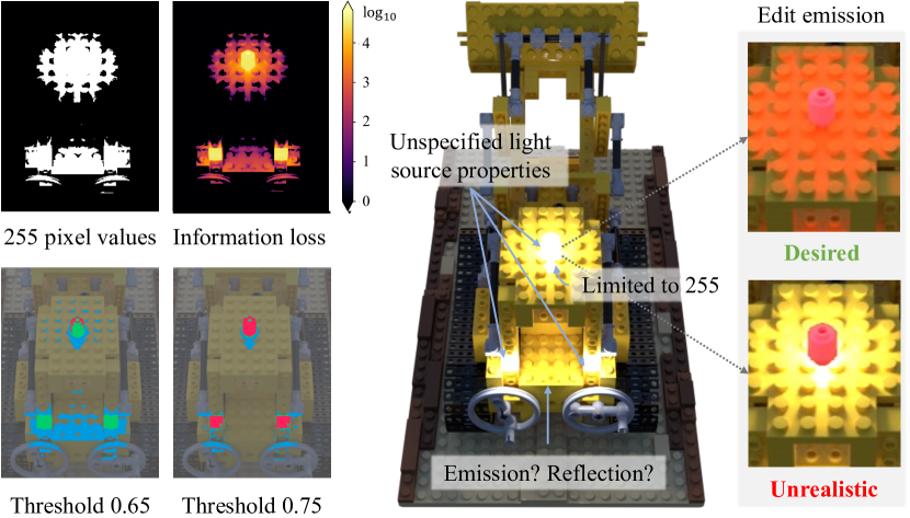
Figure 1: Challenges posed by emissive sources in LDR images. Green, red, and blue in thresholded images respectively show true positives, false negatives, and false positives of source identification. Thresholding values are scaled down divided by 255. The contrast between light on and off pixel values is more pronounced in surroundings than emissive sources. Inaccurate reconstruction of emissive sources disrupts scene editing, causing reflection areas to stay static while only the source colors change.

To address these challenges, we introduce ESR-NeRF (Emissive Sources Reconstructing NeRF), a novel approach capable of reconstructing any number of emissive sources by progressively discovering reflection areas. We assume that the scenes are observed in two lighting conditions: one with all emissive sources active and the other with them inactive. Our approach utilizes neural networks as learnable functions for representing ray-traced fields. By training networks to satisfy each light transport segment, we sidestep the computational overhead of ray tracing associated with ray bounces. In this work, we exclusively use low dynamic range (LDR) images, setting us apart from prior mesh-based methods that rely on high dynamic range (HDR) images [79, 48, 19, 2].

Our experiments encompass synthetic and real scenes, ranging from single to multiple lighting configurations with complex reflections. The scenes vary in light source counts, color, and intensity. Qualitative and quantitative evaluations show ESR-NeRF’s superiority over state-of-the-art NeRF-based re-lighting methods. Furthermore, Chamfer Distance (CD) metrics on the DTU dataset [23] indicate ESR-NeRF’s competitive performance in scene reconstruction, even without emissive sources.

We summarize our contributions as follows.

1. Our work presents the first NeRF-based inverse rendering that can deal with the scenes with any number of emissive sources, challenging the distant light assumption of previous research.

2. Unlike existing mesh-based methods relying on HDR images, we use LDR images for the first time, overcoming the poor representation of emissive sources.

3. We provide a benchmark dataset designed to evaluate the performance of emissive source reconstruction.

4. Our method is applicable to the scenes with or without emissive sources, achieving superior mesh reconstruction results on the DTU dataset.

2 Related work

Neural Rendering. Advancements in implicit representations [52, 62] and volume rendering [39] have significantly enhanced neural rendering capabilities, enabling the reconstruction of scene components from 2D images. One of the key directions is mesh extraction [80, 81, 100, 73, 44, 83], with methods like NeuS [71] and VolSDF [90] utilizing signed distance function (SDF) values for volume rendering. Recently, the efficient computation of volume rendering has become a focal point due to the substantial computational cost associated with network inference for ray color calculation [41, 49, 91]. Several methods propose to directly predict ray color using the 4D light fields concept [1, 57, 53] or leveraging voxel grids for fast inference of spatial features [12, 14, 58, 5, 31, 11]. NeuralRadiosity [17] shares similarity with our method, as it predicts ray-traced values instead of explicitly tracing individual rays. However, they primarily focus on calculating the final object color when all scene information is available. In contrast, our inverse rendering approach aims to reconstruct emissive sources within a scene, addressing the ambiguities introduced by their presence in LDR images.

Inverse Rendering. A growing emphasis revolves around the decomposition of materials represented by spatially varying bidirectional reflectance distribution functions (SVBRDF) [86, 102, 46]. To lessen the computational burden in inverse rendering [55, 101, 99, 25], several methods have adopted neural networks as lookup tables [9] or computational caches [55, 98, 93]. While NeRV [55] utilizes caching visibility and NeILF++ [93] adopts caching surface point radiance with the inter-reflection loss for incident radiance, our method diverges by focusing on tracing radiance origins. Specifically, we aim to identify emissive sources within a scene, moving beyond the simplification of incident radiance calculations. Several methods rely on diverse known lighting configurations to exploit variations in object appearances [61, 87, 66, 92]. Toggling emissive sources on and off resembles the common one-light-at-a-time (OLAT) technique, as seen in NLT [97] and ReNeRF [85]. However, our setting does not need to know light source properties and to toggle lights individually. Instead, we allow for toggling all lights together. Recent works have also jointly reconstruct the mesh, materials, and lighting [59, 42, 20, 35]. They tackle with images captured under a single unknown lighting condition [95, 98], assuming that radiance already encodes global illumination [99, 78]. However, they confine to the scenes illuminated by far-distant lights, constrained to an 8-bit color spectrum. Our work considers the presence of multiple emissive sources within a scene captured in LDR images, questioning the prevailing notion that radiance fields trained with the image rendering loss faithfully represents global illumination. While some methods [79, 48, 32, 19, 2] deal with the scenes featuring emissive sources, they work outside the volume rendering framework and depend on HDR input images, assuming prior knowledge of scene geometry.

	Voxurf	TensoIR	Path Tracing	ESR-NeRF
Big O	n	$n\cdot d$	$(n\cdot d)^{b+1}$	$n^{2}\cdot d$
Indirect illumination	✘	✔	✔	✔
BRDF decomposition	✘	✔	✔	✔
Emissive source control	✘	✘	✔	✔

Table 1: Computational cost comparison for inverse rendering methods. $n$ is the number of sampled points along a ray, $d$ is the number of scattering rays, and $b$ is the number of ray bounces.

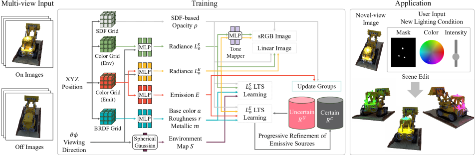
Figure 2: The pipeline of emissive source reconstruction. Given LDR images with emissive sources on and off, scene components are reconstructed by synthesizing training images and enforcing LTS requirements. Emissive sources are progressively refined via categorizing training rays into uncertain and certain groups. The scenes can be edited with new lighting conditions using reconstructed emissive sources.

3 Preliminaries

Surface Representation. Analgous to NeRF [40], neural network $f_{\theta}$ predicts SDF values at arbitrary 3D spatial locations. NeuS [71] integrates surface representation into volume rendering using the SDF-based opacity $\rho(x)=\max(\frac{-\frac{d\Phi_{s}}{dx}\left(f(x)\right)}{\Phi_{s}\left(f(x)\right)},0)$. Here $\Phi_{s}(x)=\left(1+e^{-sx}\right)^{-1}$ is the sigmoid function where $s$ controls the sharpness of surfaces. The color of a ray can be calculated as

$$\small\hat{C}(r)=\int_{0}^{\infty}T(r(t))\rho(r(t))L_{o}(r(t),\omega_{o})\,dt,$$ (1)

where $\hat{C}(r)$ denotes the predicted ray color, $r(t;c,\omega_{o})=c-t\cdot\omega_{o}$ is the ray with camera center $c$ along direction $\omega_{o}$, $T(r(t))=\exp{(\int_{0}^{t}-\rho(r(u))\,du)}$ is the transmittance, and $L_{o}(r(t),\omega_{o})$ is the outgoing radiance. Henceforth, we use $x$ to denote a point in $r(t;c,\omega_{o})$ for notational simplicity.

Light Transport in Volume Rendering. Extracting light sources necessitates analyzing the causes affecting the final ray colors. Kajiya’s rendering equation [26] factorizes the outgoing radiance $L_{o}(x,\omega_{o})$ into emission and reflections:

$$\small L_{o}(x,\omega_{o})=E(x)+\int_{\Omega}L_{i}(x,\omega_{i})R(x,\omega_{o},\omega_{i};b)d\omega_{i},\vspace{-2pt}$$ (2)

where $E(x)$ is the emission, $R(x,\omega_{o},\omega_{i};b)$ represents the SVBRDF parametrized by parameters $b$ with Lambert cosine multiplied, and $L_{i}(x,\omega_{i})$ is the incident radiance. In volume rendering, computing the incident radiance at point $x$ is akin to evaluating Eq. 1, with $x$ serving as the camera center. By iteratively factorizing the outgoing radiance in the incident radiance, the contribution of a path length $i$ for a pixel can be decomposed as in Eq. 3, where $\mathcal{H}_{i}=\Pi_{j=1}^{i-1}T(x_{j})\rho(x_{j})R(x_{j},\omega_{j-1},\omega_{j})$ is the path throughput, $S(\omega_{i})$ is the environment map strength in direction $\omega_{i}$, and $V(x,\omega_{i})=exp{\left(\int_{0}^{\infty}-\rho(r(u;x_{i},-\omega_{i}))\,du\right)}$ is the visibility of the environment map at point $x$ along direction $\omega_{i}$:

$$P_{i} =\int_{l_{1}}\int_{\Omega}\cdots\int_{l_{i-1}}\int_{\Omega}(\int_{l_{i}}T(x_{i})\rho(x_{i})E(x_{i})\,dt_{i}+$$ (3)

$$S(\omega_{i-1})V(x_{i-1},\omega_{i-1}))\mathcal{H}_{i}dt_{1}d\omega_{1}\cdots dt_{i-1}d\omega_{i-1}.$$

Extending the analysis to longer light paths, or equivalently, increasing the number of ray bounces, leads to exponential growth in computation complexity. This poses a challenge when attempting to decompose the influence of unknown emissive sources, as their ability to produce strong reflections makes ignoring indirect illumination infeasible.

4 Methodology

None of the previous works address the reconstruction of emissive sources from LDR multi-view images. Sec. § 4.1 through § 4.5 detail our method, ESR-NeRF, which reconstructs emissive sources without prior knowledge of scene geometry, materials, or lighting specifics (including their location, number, or colors). We also show how these reconstructed sources can be used for scene editing in § 4.5.

4.1 Learnable Tone-mapper

Throughout the paper, we use $\mathcal{R}$ to represent camera rays, $C$ for pixel values, and a binary flag $\mathbb{I}$ to indicate whether an image is captured with emissive sources on or off.

To extract HDR values from LDR images, we employ the softplus activation for outgoing radiance prediction and apply a clipping and gamma function $\tau$ [21] for the rendering loss such that $\hat{C}_{\tau}(r)=\tau(\hat{C}(r))$. Unlike previous NeRF-based works [55, 25, 37, 59] that limit radiance to the range of $\left[0,1\right]$, our approach allows for any positive radiance values. Yet, it creates difficulties in differentiating between the surface weight $T(x)\rho(x)$ and the magnitude of radiance value $L_{o}(x,\omega_{o})$, since it allows for the possibility of assigning extreme radiance to the points with low surface weights to render same ray colors. Such ambiguity poses challenges, particularly in dark and high-contrast scenes, aggravating surface reconstruction (see Fig. 3). To address this, we introduce a learnable tone-mapper $m_{\theta}:\mathbb{R}^{3}_{+}\rightarrow\left[0,1\right]^{3}$, that takes positionally encoded HDR linear values as input:

$$\small\hat{C}_{m_{\theta}}(r)=\int_{0}^{\infty}T(x)\rho(x)m_{\theta}(L_{o}(x,\omega_{o}))\,dt,\vspace{-2pt}$$ (4)

$$\small L_{o}(x,\omega_{o})=L_{o}^{S}(x,\omega_{o})+L_{o}^{E}(x,\omega_{o})\cdot\mathbb{I},$$ (5)

where $L_{o}^{S}(x,\omega_{o})$ is radiance when emissive sources are turned off, while $L_{o}^{E}(x,\omega_{o})$ stands for radiance added to the scene by emissive sources. Our rendering loss is then formulated as follows, with $\lambda_{\tau}$ as a hyper-parameter:

$$\small\mathcal{L}_{\text{render}}=\sum_{r\in\mathcal{R}}(\lVert C(r)-\hat{C}_{m_{\theta}}(r)\rVert_{2}^{2}+\lambda_{\tau}\lVert C(r)-\hat{C}_{\tau}(r)\rVert_{2}^{2}).\vspace{-2pt}$$ (6)

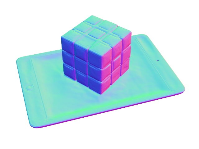
(a) Image

(b) w/o $m_{\theta}$

(c) ESR-NeRF

Figure 3: Reconstructed surfaces with the learnable tone-mapper.

4.2 Learning of Light Transport Segments

The computational complexity of object appearance analysis in volume rendering is notably high, as shown in Eq. 3. We take an alternative approach by leveraging neural networks to represent ray-traced fields, rather than explicitly tracing every rays. Our distinct contribution to inverse rendering lies in precise adjustment of radiance. Specifically, we impose constraints on the predicted radiance to satisfy each light transport segments. The light transport segments (LTS) loss, $\mathcal{L}_{lts}$, plays a pivotal role in our method:

$$\small\mathcal{L}_{lts}^{S}=\sum_{x,\omega_{o}}\lVert L_{o}^{S}(x,\omega_{o})-\hat{L}_{o}^{S}(x,\omega_{o})\rVert_{2}^{2},$$ (7)

$$\small\mathcal{L}_{lts}^{E}=\sum_{x,\omega_{o}}\lVert L_{o}^{E}(x,\omega_{o})-\hat{L}_{o}^{E}(x,\omega_{o})\rVert_{2}^{2},$$ (8)

$$\hat{L}_{o}^{S}(x,\omega_{o})=\int_{\Omega}\underbrace{S(\omega_{i})V(x,\omega_{i})R(x,\omega_{o},\omega_{i})}_{\text{direct illumination by an environment map}}\,d\omega_{i}+$$ (9)

$$\int_{\Omega}\int_{0}^{\infty}\underbrace{T(x^{\prime})\rho(x^{\prime})L_{o}^{S}(x^{\prime},-\omega_{i})\,dt^{\prime}R(x,\omega_{o},\omega_{i})}_{\text{indirect illumination by an environment map}}\,d\omega_{i}.\$$

$$\hat{L}_{o}^{E}(x,\omega_{o})=\underbrace{E(x)}_{\text{emission}}+$$ (10)

$$\int_{\Omega}\int_{0}^{\infty}\underbrace{T(x^{\prime})\rho(x^{\prime})L_{o}^{E}(x^{\prime},-\omega_{i})\,dt^{\prime}R(x,\omega_{o},\omega_{i})}_{\text{direct \& indirect illumination by emissive sources}}\,d\omega_{i}.$$

We ensure consistency between the radiance directly predicted by the network $L_{o}(x,\omega_{o})$ and the radiance achievable based on the scene context $\hat{L}_{o}(x,\omega_{o})$. Previous approaches have focused on matching $\hat{L}_{o}(x,\omega_{o})$ to training views, overlooking the relations to $L_{o}(x,\omega_{o})$. This hinders the restoration of HDR radiance by supervising scene components to LDR training views. In contrast, our LTS loss enables volumetric energy transfer of radiance, adjusting outgoing radiance based on their interrelations.

To implement this concept, we train six dedicated networks for SDF $f(x)$, SVBRDF parameters $b(x)$, emission $E(x)$, environment map $S(\omega_{i})$, outgoing radiances $L^{S}_{o}(x,\omega_{o})$ and $L^{E}_{o}(x,\omega_{o})$, to adhere to these LTS requirements. For the environment map, we represent it using 48 Spherical Gaussians [70] : $\sum_{k=1}^{M}\mu_{k}e^{\lambda_{k}(\omega_{i}\cdot\xi_{k}-1)}$, followed by the softplus activation. $\mu\in\mathbb{R}^{3}$, $\lambda\in\mathbb{R}_{+}$, and $\xi\in\mathbb{S}^{2}$ respectively denote the lobe amplitude, sharpness, and axis.

4.3 Progressive Discovery of Reflection Areas

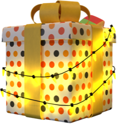
Figure 4: Left: Image with active emissive sources. Right: Identified emissive sources w/o progressive discovery of reflection areas.

Relying solely on LTS is insufficient for addressing ambiguity arising from low pixel values of emissive sources and intense reflections in adjacent regions, often leading to confusion between emission and reflection. The right image in Fig. 4 shows self-emitting objects restored with the naive LTS loss. While emissive sources are small, large areas affected by them are also identified as emissive sources. We propose a reflection-aware progressive approach for precise identification of emissive sources. By leveraging LTS learning, we extend the regions that can be regarded as reflection areas. Fig. 5 illustrates our progressive algorithm.

Reflection-Aware Emission Refinement. Since surface points are unknown and are updated during learning, we opt to utilize rays rather than surface points. This process involves categorizing training rays into two groups: uncertain ($\mathcal{R}^{U}$) and certain ($\mathcal{R}^{C}$). The certain group contains the rays confidently identified as reflection, aiding the transfer of radiance energy to nearby points. For the points in the certain group, we use the Eq. 11 instead of Eq. 10 to exclusively attibute outgoing radiances to reflections. Satisfying the LTS loss on the certain group results in adjusting the outgoing radiances of influential points, as illustrated in Fig. 5(a):

$$\small\hat{L}_{o}^{E}(x,\omega_{o})=\int_{\Omega}\int_{0}^{\infty}T(x^{\prime})\rho(x^{\prime})L_{o}^{E}(x^{\prime},-\omega_{i})\,dt^{\prime}R(x,\omega_{o},\omega_{i})\,d\omega_{i}.$$ (11)

The uncertain group includes the rays indicating the areas that are undetermined yet as reflection or emission. Using Eq. 12 to compute $\hat{L}_{o}^{E}(x,\omega_{o})$, this group adjusts emissions $E(x)$ based on the radiance updates by the certain group, where “sg” represents the stop-gradient:

$$\hat{L}_{o}^{E}(x,\omega_{o})=E(x)+$$ (12)

$$\text{sg}\left(\int_{\Omega}\int_{0}^{\infty}T(x^{\prime})\rho(x^{\prime})L_{o}^{E}(x^{\prime},-\omega_{i})\,dt^{\prime}R(x,\omega_{o},\omega_{i})\,d\omega_{i}\right).$$

As shown in Fig. 5(b), this leads to increased emissions for the regions whose radiances are adjusted to account for the reflections in the certain group. Conversely, emissions decrease for the regions where there is little change in outgoing radiance, but incident radiances are increased by surrounding influential points.

Ray Group Management. As emissions and radiances are adjusted, the groups are dynamically updated at predefined training intervals through the following process. Within the uncertain group, we evaluate the expected emission strength of rays, retaining only those above a threshold $k_{i}$. Rays below this threshold are then merged to the certain group:

$$\small\mathcal{R}^{U}_{i}=\{r|\max_{RGB}\left(\int_{0}^{\infty}T(x)\rho(x)E(x)\,dt\right)\geq k_{i},r\in\mathcal{R}^{U}_{i-1}\},$$ (13)

$$\small\mathcal{R}^{C}_{i}=\left(\mathcal{R}^{U}_{i-1}-\mathcal{R}^{U}_{t}\right)\cup\mathcal{R}^{C}_{i-1}.$$ (14)

Subsequently, newly added rays to the certain group can be used to localize influential points and update their outgoing radiances. This iterative process progressively refines the separation between reflective and emissive regions, attaining more accurate identification of emissive sources.

LTS Loss Decomposition. The LTS loss, as detailed in Eq. 15, can be decomposed using a stop-gradient operation to refine the adjustment process.

$$\mathcal{L}_{lts}^{E}=\sum_{x,\omega_{o}}( \lambda_{l}\lVert\text{sg}(L_{o}^{E}(x,\omega_{o}))-\hat{L}_{o}^{E}(x,\omega_{o})\rVert_{1}+$$ (15)

$$\lambda_{r}\lVert L_{o}^{E}(x,\omega_{o})-\text{sg}(\hat{L}_{o}^{E}(x,\omega_{o}))\rVert_{1}).$$

We prioritize $\lambda_{l}$ to enhance the update of scene context, affecting other points’ radiance given the predicted $L_{o}(x,\omega_{o})$. $\lambda_{r}$ prevents severe deviation of every $L_{o}(x,\omega_{o})$ within the current scene context. This aligns with our focus on HDR source reconstruction from LDR images, addressing under-represented information in training data.

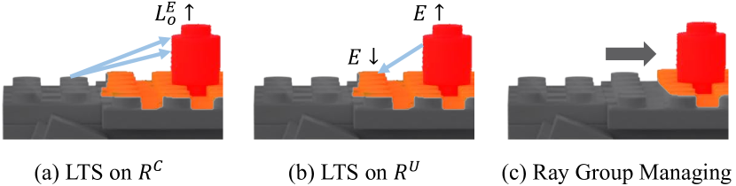
Figure 5: Illustration of the progressive emissive source reconstruction with reflection awareness. Gray color represents the areas belonging to the certain group, while the red (emissive sources) and orange (their reflections) areas belong to the uncertain group.

4.4 Training Details

We employ the Voxurf architecture [83] as backbone and adopt the simplified Disney BRDF model [10] for SVBRDF representation, with parameters including base color $\in[0,1]^{3}$, roughness $\in[0,1]$, and metallic $\in[0,1]$. The learnable tone-mapper, structured as a two-layer MLP, is utilized for the rendering loss only. Initially, we pre-train our networks using the rendering loss, subsequently integrating the basic LTS loss (Eq. 7 and Eq. 8) into our training regimen. This phase transitions to the reflection-aware progressive training scheme, where we adopt the $\ell_{1}$ loss due to its empirical stability in refining emissive source reconstruction. We use a smoothing regularization to promote local consistency in normals, BRDFs, and emissions. To ensure view-consistent labeling of 3D points as either reflective or emissive, we implement the emission suppression loss for points beloning to the certain group:

$$\small\mathcal{L}_{supp}^{E}=\sum_{r\in R_{t}^{C}}\lVert\int_{0}^{\infty}T(x)\rho(x)E(x)\,dt\rVert_{2}^{2},$$ (16)

The threshold $k_{i}$ linearly increases with each time step $t$, utilizing a grid search within a range of $[10^{-3},10^{-5}]$ to find the slope. We construct mini-batches via stratified sampling within each group. For a detailed description of our training procedure, please refer to Appendix.

	White colored												Vivid colored
	Lego		Gift		Book		Cube		Billboard		Balls		Lego		Gift		Book		Cube		Billboard		Balls
	IoU	MSE	IoU	MSE	IoU	MSE	IoU	MSE	IoU	MSE	IoU	MSE	IoU	MSE	IoU	MSE	IoU	MSE	IoU	MSE	IoU	MSE	IoU	MSE
Twins	0.22	20.19	0.49	8.59	0.63	3.91	0.95	31.83	0.69	1.12	0.90	0.06	0.25	6.96	0.24	6.09	0.55	2.63	0.95	10.64	0.09	0.75	0.83	0.04
NeILF++	0.43	20.88	0.07	9.38	0.95	4.64	0.93	32.67	0.01	1.95	0.91	0.80	0.30	7.65	0.09	6.86	0.95	3.36	0.94	11.49	0.02	1.57	0.92	0.78
TensoIR	0.71	20.13	0.15	8.55	0.95	3.87	0.95	31.73	0.76	1.11	0.95	0.05	0.33	6.93	0.15	6.05	0.95	2.59	0.96	10.60	0.77	0.74	0.95	0.03
ESR-NeRF	0.81	8.38	0.60	3.49	0.96	1.19	0.97	17.87	0.84	0.46	0.95	0.04	0.51	5.48	0.59	2.50	0.96	0.51	0.97	7.94	0.88	0.26	0.94	0.03

Table 2: Results of emissive source identification. ESR-NeRF outperforms state-of-the-art re-lighting methods in reconstructing emissive sources, regardless of their color. The IoU measures the source area identification (a higher value is better), and the MSE quantifies the difference between reconstructed images and HDR ground truth images (a lower value is better).

4.5 Scene Editing

Reconstructed emissive sources enable scene editing; users select emissive sources using binary masks $M_{j=1\dots N}$ and specify lighting conditions using colors $c_{j=1\dots N}$ and intensities $i_{j=1\dots N}$ within the HSV color space [54].

We identify the rays in the uncertain group that match $M$ by projecting expected surface points $p$ of the rays onto the camera with the pose $\mathbf{R}|\mathbf{t}$:

$$\small p=\int_{0}^{\infty}T(x)\rho(x)x\,dt,$$ (17)

$$\small\mathbb{I}_{j}^{hit}(x)=\text{interp}(M_{j},p^{\prime})>0,\,\text{where }p^{\prime}=\mathbf{K}[\mathbf{R}|\mathbf{t}][p|1]^{T}.$$ (18)

For the rays satisfying $\mathbb{I}_{j}^{hit}(x)$, we apply the designated lighting conditions. The new emission values are computed by substituting the original hue (H) and saturation (S) of $E(x)$ with the user-specified color $c_{j}$ and adjusting the value (V) of $v(x)$ with the new intensity $i_{j}$:

$$\small E(x)=\text{hsv\_to\_rgb}\left(\left[c_{j}|\left(v(x)\times i\right)\right]\right)\cdot\mathbb{I}_{j}^{hit}+E(x)\cdot\neg\mathbb{I}_{j}^{hit}.$$ (19)

These modifications influence scene appearance by optimizing the loss in Eq. 20. During this process, all networks, except for $L_{o}^{E}(x,\omega_{o})$, are frozen:

$$\vspace{-5pt}\small\mathcal{L}_{edit}=\sum_{x,\omega_{o}}\lVert L_{o}^{E}(x,\omega_{o})-\text{sg}(\hat{L}_{o}^{E}(x,\omega_{o}))\rVert_{2}^{2}.$$ (20)

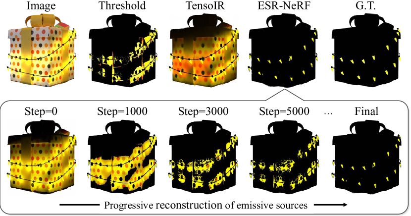
Figure 6: Comparison of identified emissive sources. ESR-NeRF excels through the reflection-aware progressive refinement.

	Image	Twins	PaletteNeRF	TensoIR	ESR-NeRF	G.T.
Lego
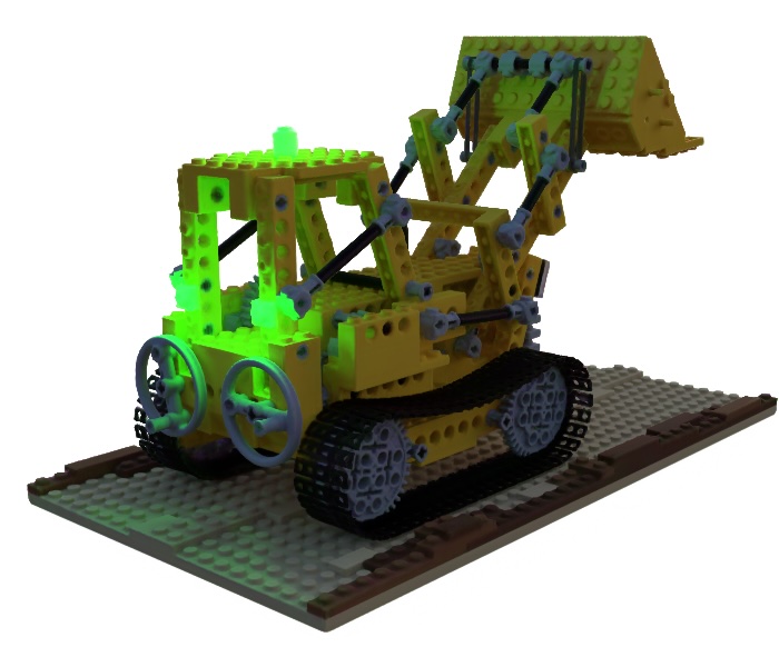
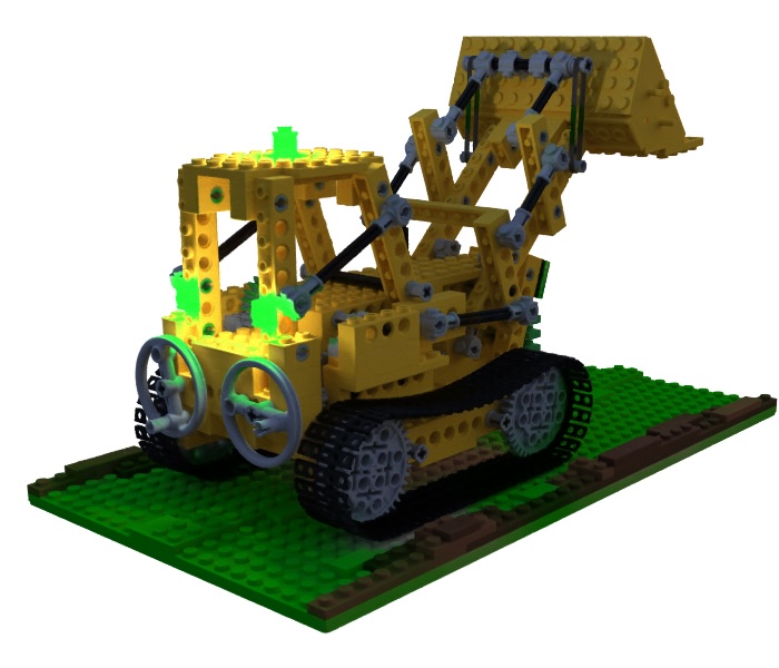
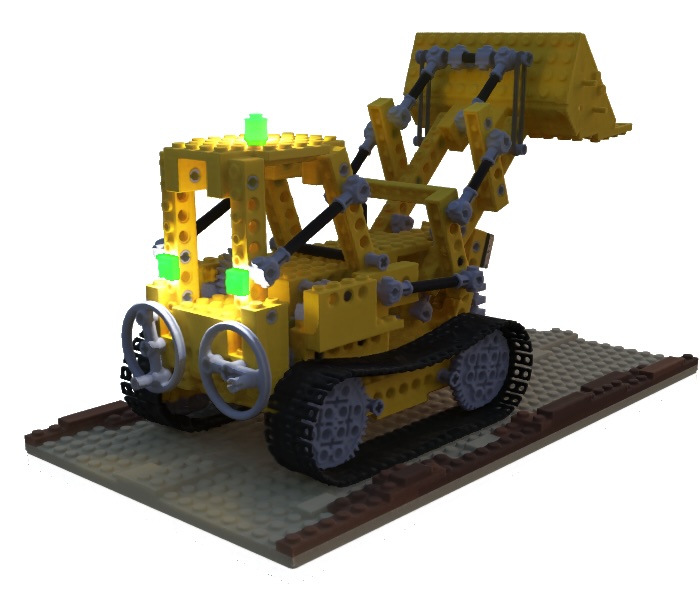
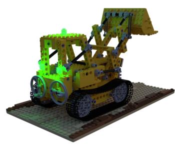
Cube
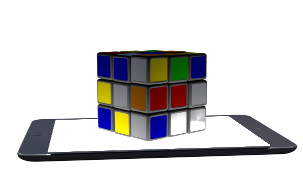
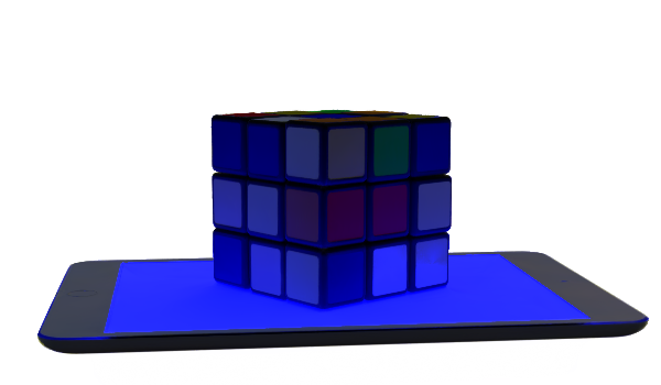
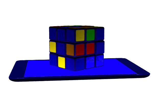
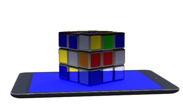
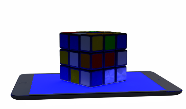
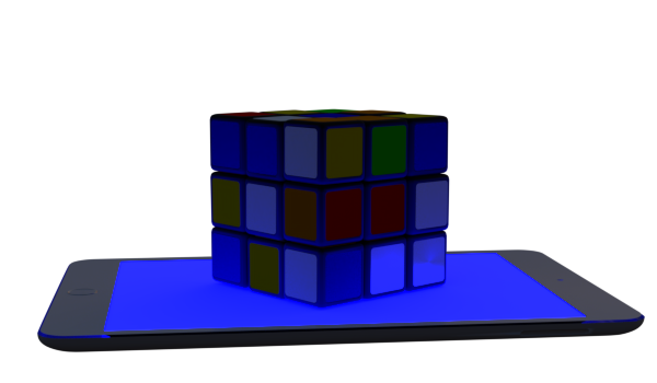
Gift

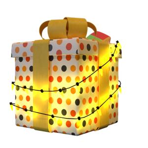
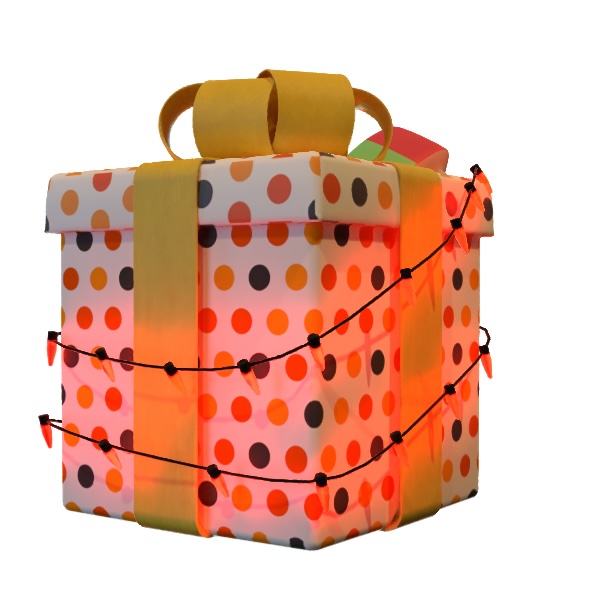
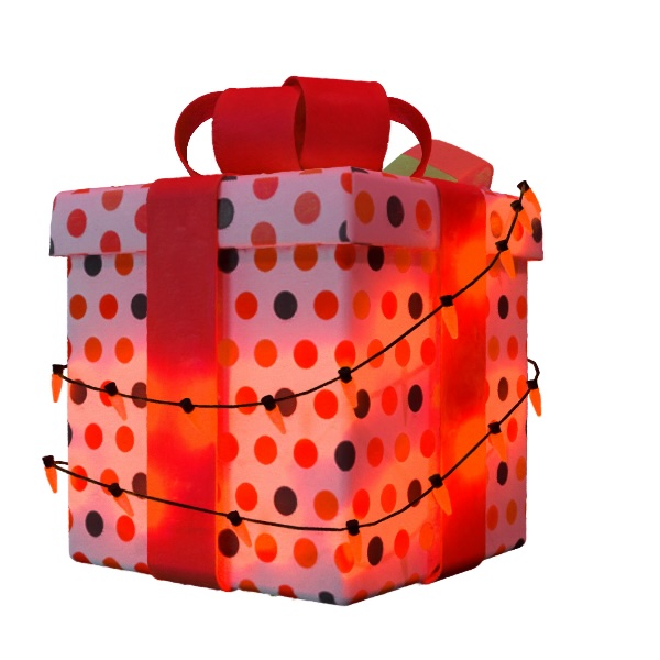
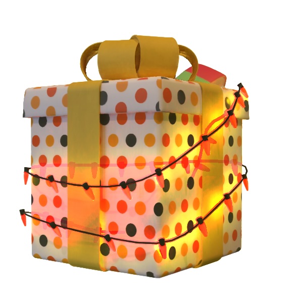
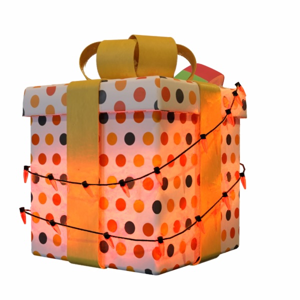
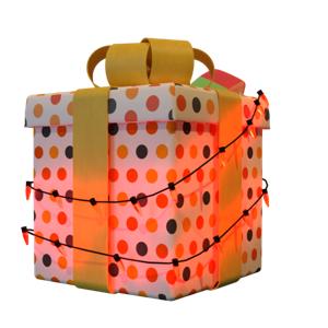
0.5pt1.5mm

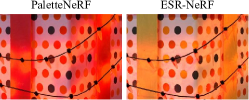
Figure 7: Comparison of scene editing. ESR-NeRF provides precise source control and faithfully represents reflection effects. For easy comparison in the Cube scene of low intensity, the bottom-right images are presented with a 40% increased brightness.

5 Experiments

We assess ESR-NeRF in reconstructing emissive sources by focusing on both identification and intensity restoration. To showcase its effectiveness, we conduct a range of experiments, including scene editing, ablation studies, illumination decomposition, and surface reconstruction, providing both quantitative and qualitative results.

5.1 Experiment Settings

We curate 6 diverse synthetic scenes, each with 200 training images evenly distributed between on and off lighting conditions. To evaluate the robustness of our approach against light colors, we consider two distinct settings of white colored and vivid colored emissive sources, resulting in a total of 12 scenes. The vivid colors are selected with full saturation in the HSV color space. We measure source identification and radiance reconstruction using IoU and MSE metrics on novel view test images, comparing against ground truth data from Blender-rendered emission masks and EXR files. The emission strengths, the maximum EXR file values, range from 2 to 200. For quantitative scene editing evaluation, we alter the white-colored sources to various colors—red, green, blue, cyan, magenta, yellow—and adjust intensities to half or double their original values. Qualitative results include scene editing for vividly colored sources and real scenes captured with a Fuji 100s camera using Philips smart bulbs as emissive sources. Quantitative assessments are based on 50 test images from novel camera poses, except for MSE measured for 25 test images. We denote the best performance with blue and the second-best with green. Additionally, we utilize the DTU dataset [23] to evaluate ESR-NeRF’s performance in surface reconstruction tasks where emissive sources are absent.

Baselines. We select two state-of-the-art re-lighting methods, TensoIR [25] and NeILF++ [93], that do not require prior lighting information. For thorough evaluation, we also implement a simple method, Twins, where separate models are trained under light on and off conditions. The Twins utilize the radiance discrepancies between the on and off models to distinguish and adjust emissive sources. For scene editing, we add NeRF-W [38] and PaletteNeRF [28] as baselines. Both NeRF-W and Twins adopt the Voxurf [83] architecture for fair comparison. For methods unable to individually control emissive sources, all sources are adjusted together to match the last lighting condition by a user. For the DTU dataset, we include state-of-the-art surface reconstruction methods that use object masks, such as NeuS [71] and Voxurf, as well as Neural-PBIR [59], that jointly reconstructs surfaces, materials, and environment maps.

	NV		NV + I		NV+ C		NV + I + C
	PSNR	LPIPS	PSNR	LPIPS	PSNR	LPIPS	PSNR	LPIPS
Twins	36.52	0.0141	27.91	0.0252	31.02	0.0252	28.21	0.0310
NeRF-W	36.44	0.0142	24.77	0.0417	-	-	-	-
NeILF++	24.40	0.0556	24.71	0.0579	24.06	0.0750	23.24	0.0770
TensoIR	38.04	0.0103	27.28	0.0418	26.36	0.0505	25.18	0.0531
PaletteNeRF	33.66	0.0233	23.27	0.0483	24.44	0.0646	22.58	0.0703
ESR-NeRF	38.79	0.0083	29.99	0.0193	31.73	0.0196	31.63	0.0199

Table 3: Scene editing results. NV: novel view synthesis, I: intensity editing, and C: color editing. A higher PSNR or lower LPIPS value is better.

5.2 Results

Emissive Source Recosntruction. Tab. 2 shows that our approach excels in accurately identifying emissive source regions and restoring their intensity, regardless of the source color. While TensoIR and NeILF++ can restore emissions by modifying their physical rendering equations, they suffer from emissive source ambiguity, leading to near-zero IoU performance (see Appendix). For a comprehensive comparison, we report the best performance of the baseline methods using thresholding on the reconstructed emission strength at 0.01 intervals. ESR-NeRF consistently outperforms the baselines in identifying emissive source regions across all scenes. Our method also achieves significantly lower MSE values for restoring LDR to HDR images compared to the baselines, demonstrating its effectiveness of handling the ill-posed nature of the scenes with emissive sources. This is visually confirmed in Fig. 6, where ESR-NeRF surpasses the baselines in a complex scene with numerous small light bulbs.

Image	Emission	Re-light (ours)	Re-light (G.T.)

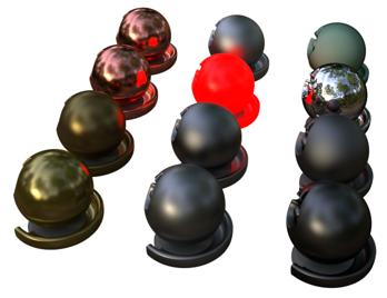
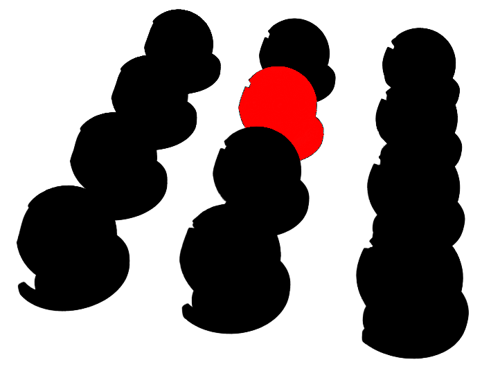
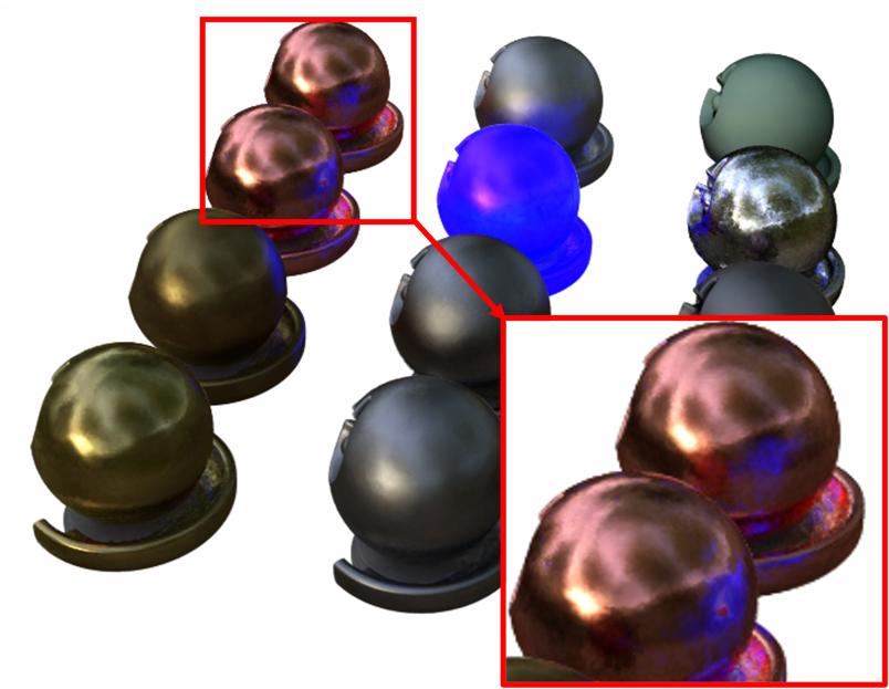
Figure 8: Reconstructed emitter and re-lighting at novel view.

Scene Editing.

	Lego	Gift	Book	Billboard
Image
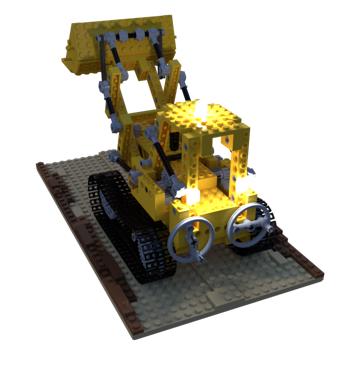
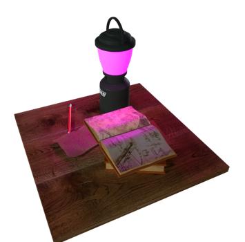
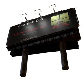
Emission
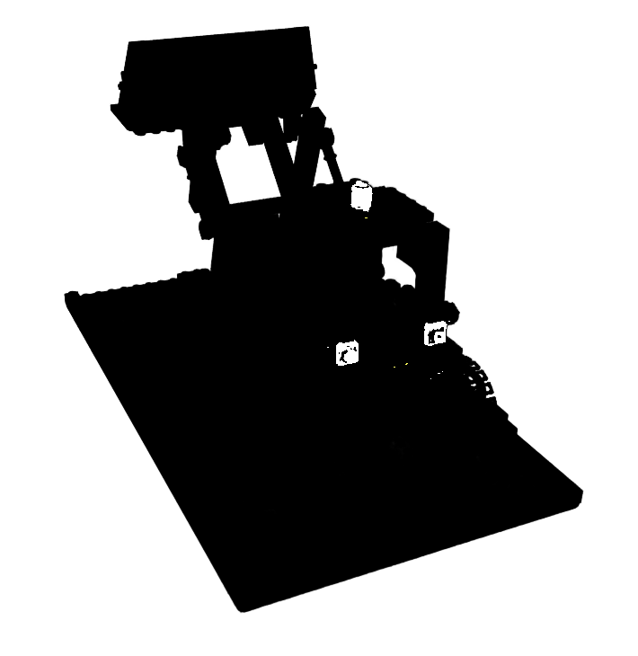
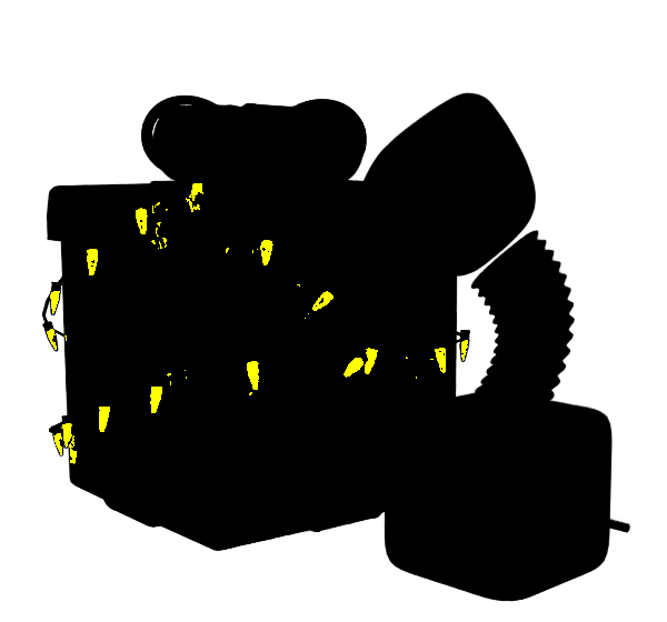
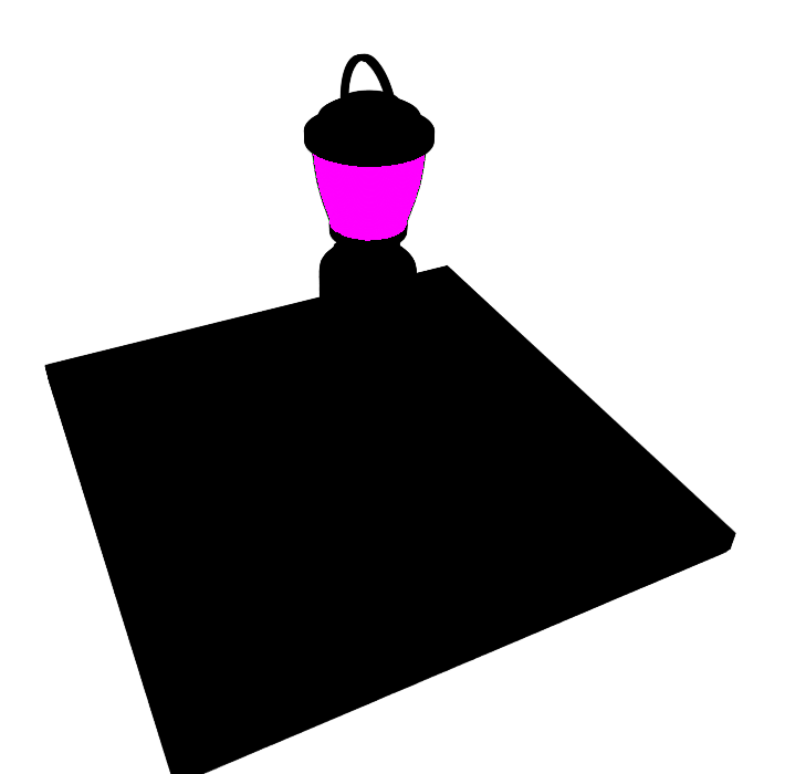
Edited

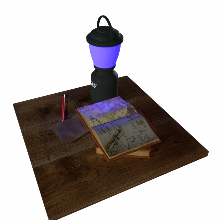
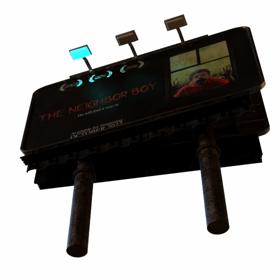
Figure 9: Results of source reconstruction and scene editing.

Tab. 3 and Fig. 7 showcase the scene editing results under novel lighting conditions. Baseline methods struggle to adapt to lighting changes due to their inability to reconstruct emissive sources accurately. For example, in the Lego scene, TensoIR fails to adjust the illumination in surrounding regions when the color of emissive sources is changed, and in the Cube scene, both the hidden iPad screen and the cube surface covered by the user input mask change together. Twins introduces blue light onto yellow and red surfaces, leading to unintended white and purple appearances, even though there should be no reflection. PaletteNeRF, which manipulates scenes through re-colorization, lacks precise control over illumination, as seen in the synchronous color changes in the yellow ribbon and lighting. In contrast, ESR-NeRF demonstrates superior performance in scene editing outshining all baselines thanks to the accurate identification of emissive sources, as detailed in Table 3. ESR-NeRF effectively balances source reconstruction and novel view synthesis, ensuring high performance in both tasks. NeRF-W is excluded from color adjustments since it doesn’t support direct color change through interpolating latent variables learned with light on and off conditions.

Fig. 8 to 9 present additional examples of emissive source reconstruction and scene editing results. Fig. 10 shows results on real scenes, for which due to the impracticality of precise control over smart bulb colors, we offer emission reconstruction results with pseudo ground truth data. Our method effectively identifies emissive sources in real scenes, while it faces challenges in capturing complex reflections within light bulbs, as evident in the bright spot at the center of the bulbs in the ground truth edit results.

Ablation Analysis. Progressive refinement with the stop-gradient operation in Eq. 15 improves the identification of emissive sources and reduces MSE values. Without $m_{\theta}$, surface reconstructions become unreliable, complicating the accurate reconstruction of emissive sources. This issue is evident from the CD metrics and illustrated in Fig. 3. Further analyses are provided in Appendix.

Illumination Decomposition. Fig. 11 demonstrates ESR-NeRF’s decomposition of scene illumination into direct and indirect lighting from an environment map, as well as emissions and their reflections. The shadow behind the yellow ribbon in the direct figure and the illumination in the indirect figure showcase ESR-NeRF’s ability to model both direct and indirect illumination. The reflection figure shows that our method accurately captures how emissive sources contribute to reflections on nearby regions.

	Image	Emission	Edited	Pseudo G.T.
Jobs
Dolls
Cosmetics

Figure 10: Source reconstruction and scene editing on real scenes.

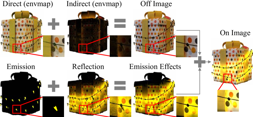
Figure 11: An example of illumination decomposition.

Surface Reconstruction. Interestingly, our approach can be applied to the scenes without emissive sources to enhance surface reconstruction, as evidenced by the lower CD values in Tab. 4 on the DTU dataset. For this experiment, we use Eq. 7 to 10 without our progressive refinement technique. ESR-NeRF’s ability to adjust interrelated outgoing radiances helps prevent surface formations where radiances cannot be produced, considering the predicted scene context. Additional visualizations of the normals, BRDF, and environment maps are provided in Appendix.

Scan	NeuS	Voxurf	Neural-PBIR	ESR-NeRF
24	0.83	0.65	0.57	0.58
37	0.98	0.74	0.75	0.71
40	0.56	0.39	0.38	0.38
55	0.37	0.35	0.36	0.33
63	1.13	0.96	1.04	0.93
65	0.59	0.64	0.73	0.57
69	0.60	0.85	0.65	0.78
83	1.45	1.58	1.28	1.18
97	0.95	1.01	0.97	0.95
105	0.78	0.68	0.76	0.58
106	0.52	0.60	0.53	0.54
110	1.43	1.11	0.84	1.08
114	0.36	0.37	0.38	0.33
118	0.45	0.45	0.46	0.40
122	0.45	0.47	0.49	0.44
mean	0.77	0.72	0.68	0.65

Table 4: Results of surface reconstruction via the Chamfer distance on the DTU dataset. A lower value is better.

	White		Vivid
	IoU $\uparrow$	MSE $\downarrow$	IoU $\uparrow$	MSE $\downarrow$
w/o progressive	0.40	9.92	0.41	3.93
w/o sg	0.71	6.45	0.60	3.47
ESR-NeRF	0.86	5.24	0.81	2.79

	DTU
	CD $\downarrow$
w/o $m_{\theta}$	0.93
w/o LTS	0.71
ESR-NeRF	0.65

Table 5: Ablation studies on the sruface reconstruction (left) and the emissive source reconstruction (right).

6 Conclusion

We present ESR-NeRF as the first NeRF-based inverse rendering method for the scenes with emissive sources. Our approach uses LDR images, eliminating the need of HDR images to reconstruct emissive sources. Furthermore, we demonstrate the application of reconstructed sources in scene editing, enabling color and intensity modifications.

Limitations. Future work could explore using a single lighting condition to disentangle emissive sources, environmental lighting, and object texture. It is also promising to address the challenge of volume ray tracing in unbounded scenes to extend to indoor scenes. Additionally, LTS based re-lighting may be weak in representing new colors that traverse unobserved light paths during training. An alternative approach could be extracting emission texture maps and modifying it using the engines such as Blender [13] or Mitsuba [22]. More details on alternative re-lighting methods and radiance fine-tuning are provided in Appendix.

7 Acknowledgements

This work was supported by Samsung Electronics MX, Basic Science Research Program through the National Research Foundation of Korea(NRF) funded by the Ministry of Education(RS-2023-00274280), and Institute of Information & Communications Technology Planning & Evaluation (IITP) grant funded by the Korea government (MSIT) (No. 2019-0-01082, SW StarLab; No. 2022-0-00156, Fundamental research on continual meta-learning for quality enhancement of casual videos and their 3D metaverse transformation). Gunhee Kim is the corresponding author.

Supplementary Material

-1

8 Appendix

8.1 Implementation Details

Training Procedure. Our implementation builds upon Voxurf [83], excluding its dual-color network feature. We adhere to the coarse and fine processing stages described in Voxurf before initiating our LTS learning-based training strategy. Additionally, we compute ray colors using alpha masks to filter out points in empty space, aligning with practices in previous studies [83, 12, 25]. The LTS learning training procedure with progressive refinement approach is:

1. Initialize ray groups: Uncertain rays $R^{U}_{0}=R$ and certain rays $R^{C}_{0}=\emptyset$.

2. Form mini-batches using stratified sampling within each ray group.

3. Calculate the rendering loss, $\mathcal{L}_{render}$.

4. For rays in the mini-batch, uniformly sample 100 points to evaluate the LTS loss, $\mathcal{L}_{lts}$.

5. Compute the surface normal at sampled points.

6. For $L_{o}^{E}(x,\omega_{o})$, sample an additional viewing direction on the upper hemisphere at these points.

7. For $\hat{L}_{o}^{E}(x,\omega_{o})$, sample 256 rays on the upper hemisphere at these points to compute incident radiance.

8. Calculate $\mathcal{L}_{lts}$, considering the group membership of each point.

9. Update network parameters.

10. Adjust ray groups at specified training intervals.

11. Repeat steps 2 through 10 until training ends.

Discretization. Following NeuS [71], we approximate ray color computation using $N$ discrete points sampled along the ray, denoted as $\{x_{i}=c-t_{i}\omega_{o}|i=1,...,N,t_{i}<t_{i+1}\}$:

$$\small\hat{C}(r)=\sum_{i=1}^{N}T_{i}\alpha_{i}L_{o}(x_{i},\omega_{o}),$$ (21)

$$\small\alpha_{i}=\max\left(\frac{\Phi_{s}(f(x_{i}))-\Phi_{s}(f(x_{i+1}))}{\Phi_{s}(f(x_{i}))},0\right),$$ (22)

$$\small T_{i}=\prod_{j=1}^{i-1}(1-\alpha_{j}).$$ (23)

$\alpha$ is the discrete equivalent of the SDF-based opacity, $\rho$.

For reflections in $\hat{L}_{o}(x,\omega)$, we employ Monte Carlo sampling, uniformly sampling directions $\omega_{i}$ around the normal $n$ at point $x$ on the upper hemisphere. While the current implementation of ESR-NeRF doesn’t include importance sampling for incident rays, incorporating it in future work for variance reduction may enhance overall performance.

$$\small\hat{L}_{o}(x,\omega_{o})=E(x)+\frac{1}{M}\sum_{j=1}^{M}\left(\frac{L_{i}(x,\omega_{j})R(x,\omega_{o},\omega_{j})}{\frac{1}{2\pi}}\right).$$ (24)

Simplified Diseny BRDF. We adopt the simplified Disney principled BRDF function [68], parameterized by base color $b$, metallic $m$, and roughness $r$.

$$R(x,\omega_{o},\omega_{i}) =\frac{D(h,n,r)F(\omega_{o},h,b,m)G(\omega_{o},\omega_{i},h,r)}{4(n\cdot\omega_{o})}$$ (25)

$$+\left(n\cdot\omega_{i}\right)\left(1-m\right)\left(\frac{b}{\pi}\right),$$

The half vector $h$ is defined as $h=\frac{\omega_{o}+\omega_{i}}{\lVert\omega_{o}+\omega_{i}\rVert_{2}}$. Following NeILF++ [93], the normal distribution function $D$ is approximated using Spherical Gaussian:

$$\small D(h,n,r)=\frac{1}{\pi r^{4}}\exp(\frac{2}{r^{4}}(h\cdot n-1)),$$ (26)

The Fresnel term $F$ is calculated as follows:

$$F(\omega_{o},h,b,m) =F_{0}+(1-F_{0})(1-(\omega_{o}\cdot h)^{5}),$$ (27)

$$\text{where }F_{0} =0.04(1-m)+bm,$$

The geometry term $G$ adopts the GGX function [10].

$$G(\omega_{o},\omega_{i},n,r) =\frac{(n\cdot\omega_{o})(n\cdot\omega_{i})}{\left((n\cdot\omega_{o})(1-k)+k\right)\left((n\cdot\omega_{i})(1-k)+k\right)},$$ (28)

$$\text{where }k =\frac{r^{2}}{2}.$$

For simplicity, our BRDF model incorporates the Lambert cosine term $(n\cdot\omega_{i})$.

Gamma Correction. To ensure HDR linear color space for outgoing radiance, we apply the standard gamma correction as defined by IEC [21] to ray colors before calculating the rendering loss. The gamma-corrected sRGB color, given a linear color $C_{\text{linear}}$, is computed as follows:

$$\tau(C_{\text{linear}})=\begin{cases}12.92C_{\text{linear}}&\text{if }C_{\text{linear}}\leq 0.0031308,\\ 1.055C_{\text{linear}}^{1/2.4}-0.055&\text{if }C_{\text{linear}}>0.0031308.\end{cases}$$ (29)

RGB to HSV. For scene editing tasks, we utilize the HSV color model [54]. The hue ($H\in[0,1]$), saturation ($S\in[0,1]$), and value ($V\in\mathbb{R}_{+}$) are calculated using the following method:

$$M =\max(R,G,B),$$ (30)

$$m =\min(R,G,B),$$

$$C =M-m.$$

$$H =(H^{\prime}/6.0)\mod 1.0,$$ (31)

$$H^{\prime} =\begin{cases}0&\text{if }C=0,\\ \frac{G-B}{C}&\text{if }M=R,\\ \frac{B-R}{C}+2&\text{if }M=G,\\ \frac{R-G}{C}+4&\text{if }M=B.\end{cases}$$

$$\small S=\begin{cases}0&\text{if }V=0,\\ \frac{C}{V}&\text{otherwise},\end{cases}$$ (32)

$$\small V=\max(R,G,B)$$ (33)

HSV to RGB. Once the color is replaced and intensity is adjusted in the HSV space, the conversion back to RGB is performed as:

$$m =V-C,$$ (34)

$$H^{\prime} =H\times 6.0,$$

$$C =S\times V,$$

$$X =C\times(1-\lvert H^{\prime}\mod 2-1\rvert),$$

$$(R^{\prime},G^{\prime},B^{\prime}) =\begin{cases}(C,X,0)&\text{if }0\leq H^{\prime}<1,\\ (X,C,0)&\text{if }1\leq H^{\prime}<2,\\ (0,C,X)&\text{if }2\leq H^{\prime}<3,\\ (0,X,C)&\text{if }3\leq H^{\prime}<4,\\ (X,0,C)&\text{if }4\leq H^{\prime}<5,\\ (C,0,X)&\text{if }5\leq H^{\prime}<6.\end{cases}$$

$$\small(R,G,B)=(R^{\prime}+m,G^{\prime}+m,B^{\prime}+m).$$ (35)

8.2 Dataset Details

Dataset Construction. This section outlines the dataset used for training and evaluation. Each scene in our dataset comprises 200 training images, with an equal split between two lighting conditions: “on” and “off”. Emission masks are utilized as ground truth for emissive source identification, while EXR files with linear pixel values assess the accuracy of the reconstructed strength of emission and reflection. All data are rendered using the Cycles path tracing in Blender [13], with settings that could artificially alter scene illumination are disabled, such as incdient light clamping and the Filmic transform. For scene editing under novel lighting conditions, we introduce a variety of test scenarios, including intensity editing, color editing, and combined intensity and color editing, each with 50 images. We derive these scenarios from 25 unique camera positions from the novel view evaluation dataset, each under two different lighting conditions, Intensity adjustments are made relative to the original scene’s emissive source strength, with “0” indicating “light off” and “1” matching the “light on” intensity. We test intensity adjustments at half (0.5) and double (2.0) the original levels. In scenes allowing individual source adjustments, we include an additional intensity condition where lights are selectively turned off (0.0). For color editing, we select six colors—red, green, blue, cyan, magenta, and yellow—to demonstrate the effects of various light source colors on scene illumination.

Scene Characteristics. Our scenes are meticulously crafted using assets from Blendswap and cgtrader, with licensing details and the count of emissive sources detailed in Tab. 6. Below, we describe the unique aspects of each scene.

Scene Name	Num Lights	License
Lego	3	By Heinzelnisse (CC-BY-NC): https://www.blendswap.com/blend/11490
Gift	29	By juan215 (Royalty Free):
		https://www.cgtrader.com/free-3d-models/household/household-tools/gift-box-aeb8f01e-929f-4041-9117-bcea21f3c813
		By MiriamAHoyt (CC-0): https://blendswap.com/blend/21434
Book	1	By lakerice (CC-0): https://blendswap.com/blend/22197
		By 3dfiles (CC-BY): https://blendswap.com/blend/28034
		By bloknayrb (CC-BY): https://www.blendswap.com/blend/26172
Cube	1	By 4NDR31JK (CC-BY): https://www.blendswap.com/blend/30149
		By sriniwasjha (CC-BY): https://blendswap.com/blend/18409
Billboard	6	By M0h4wkAD3 (CC-BY-NC-SA): https://blendswap.com/blend/27481
Balls	1	By elbrujodelatribu (CC-0): https://blendswap.com/blend/10120

Table 6: Number of emissive sources and licenses of objects used in scenes.

• LEGO: This scene showcases three emissive sources, all starting with the same color and intensity. The intricate designs of the LEGO bricks create complex reflection effects. The emissive sources in these scenes are tested for both collective and individual adjustments.

  

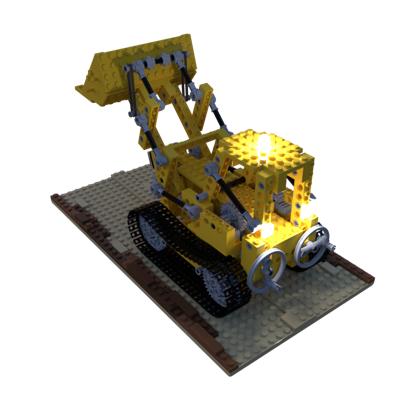
  (a) Lego (white)

  

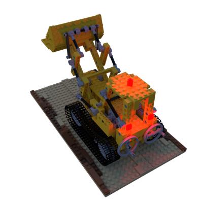
  (b) Lego (vivid)

• Gift: Featuring a gift box, a toy, and numerous small bulbs, this scene presents a challenge with its multitude of tiny light bulbs and extensive reflection areas.

  

  (a) Gift (white)

  

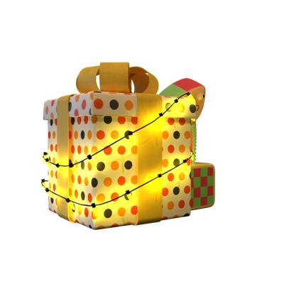
  (b) Gift (vivid)

• Book: The Book scene features a single large light source consisting of a lamp, a book, and a pencil. The emphasis here is on identifying and restoring the very large emissive source.

  

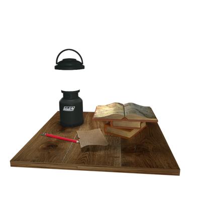
  (a) Book (white)

  

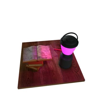
  (b) Book (vivid)

• Cube: Comprising a tablet PC and a cube, this scene is marked by its sophisticated reflection effects, especially on the cube surfaces which varying albedo.

  

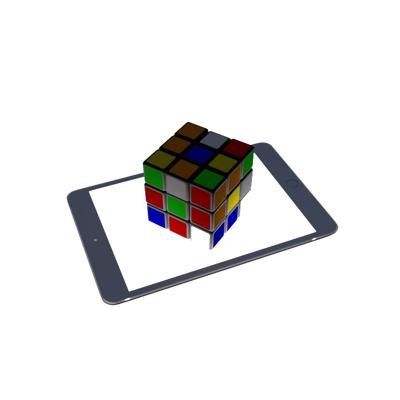
  (a) Cube (white)

  

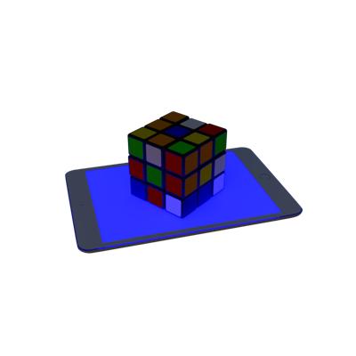
  (b) Cube (vivid)

• Billboard: This scene includes two billboards, each equipped with three emissive sources, summing up to six sources. The lights are positioned to shine downwards from the billboards’ tops. We adjust the emissive sources collectively and individually. Individual adjustments are performed for three light groups by pairing the light sources of the front and back billboards.

  

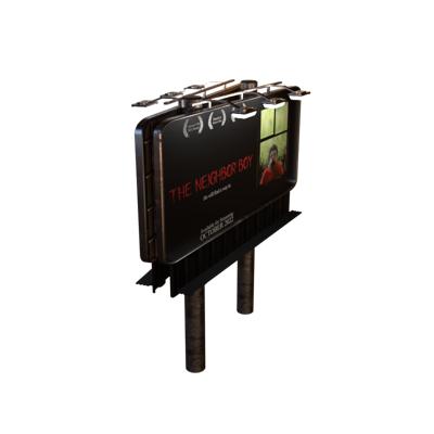
  (a) Billboard (white)

  

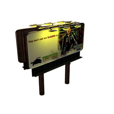
  (b) Billboard (vivid)

• Balls: This is the material balls scene in NeRF, with the modification of the red ball as an emissive source.

  

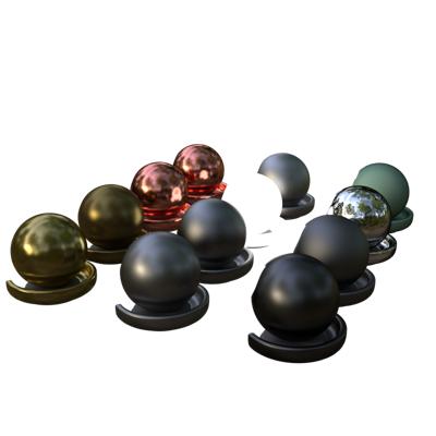
  (a) Balls (white)

  

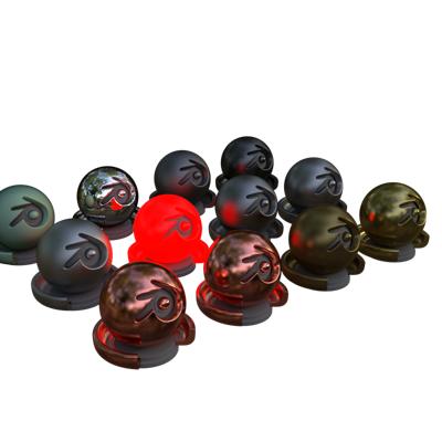
  (b) Balls (vivid)

Image	Normal	Base Color	Roughness	Metallic	Env. Map

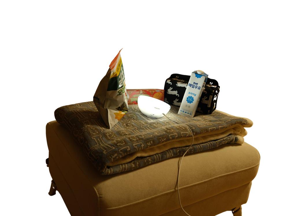
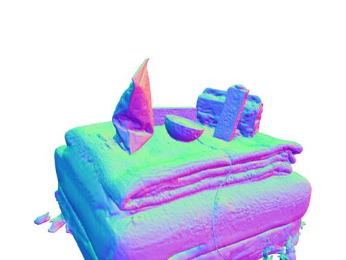
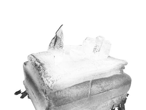
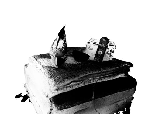
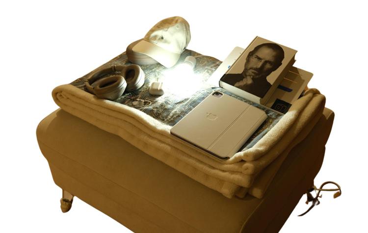
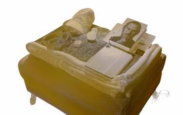
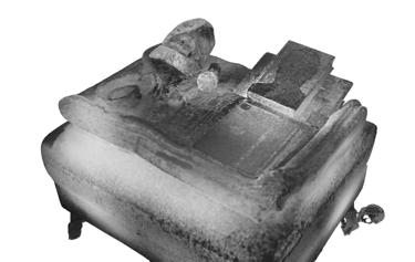
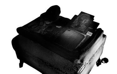
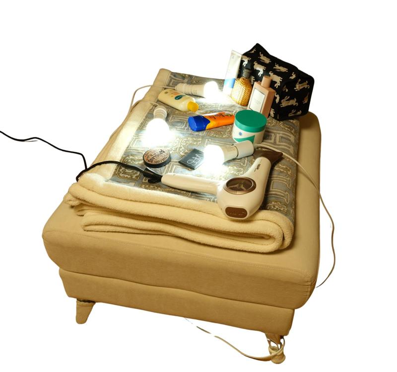
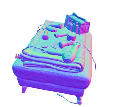
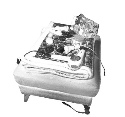
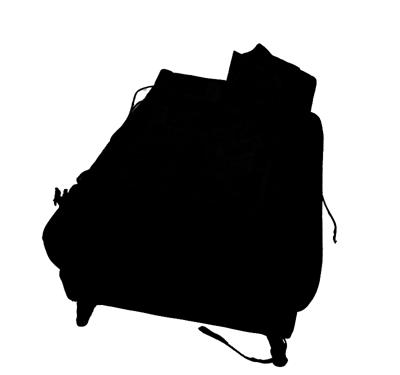
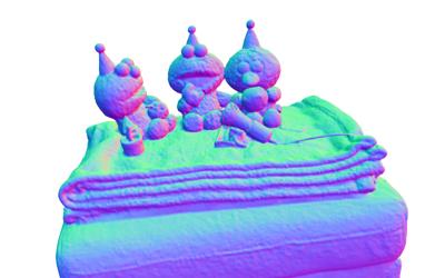
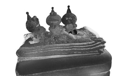
Figure 18: Decomposed scene components on real scenes

Image	Emission	Edit 1	Edit 2

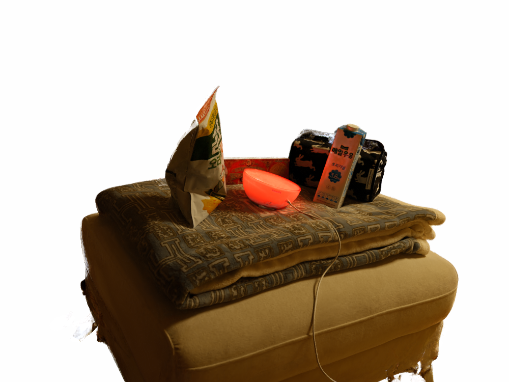
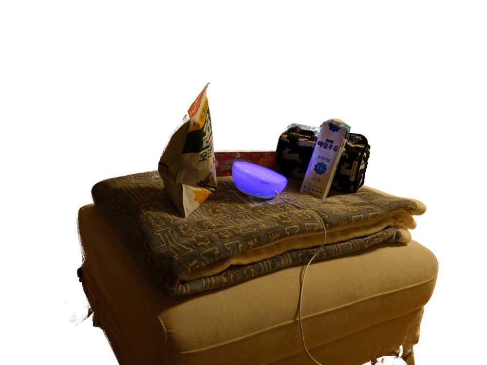
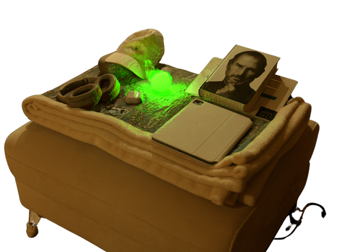
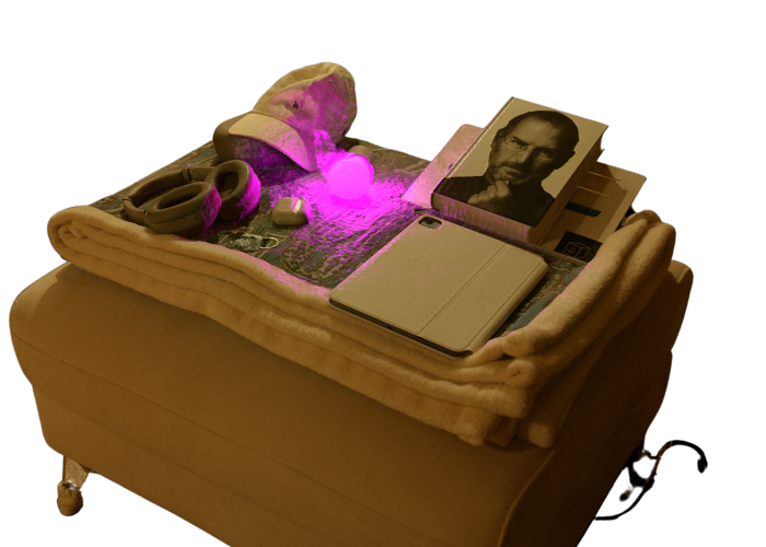
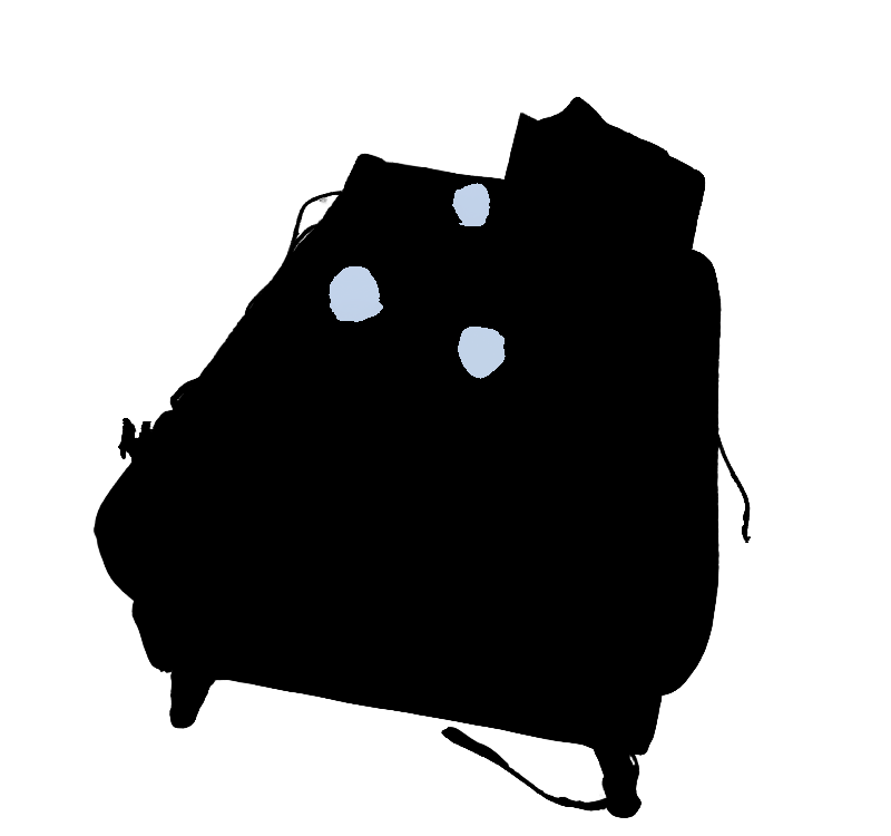
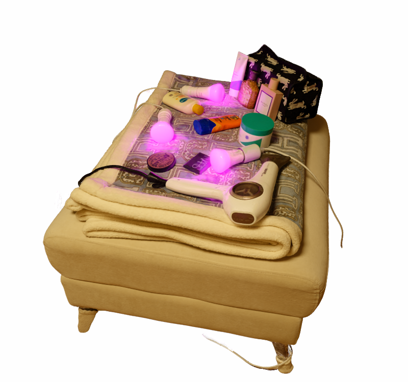
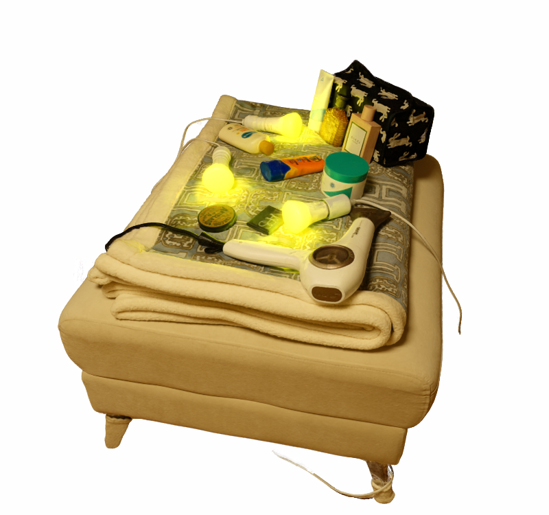
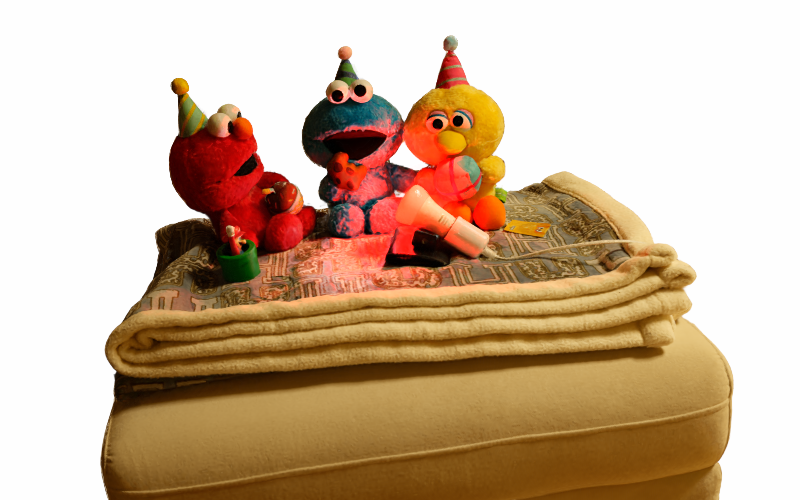
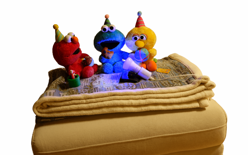
Figure 19: Identified emissive sources and edited results on real scenes.

Image	Edit	G.T.	Edit	G.T.

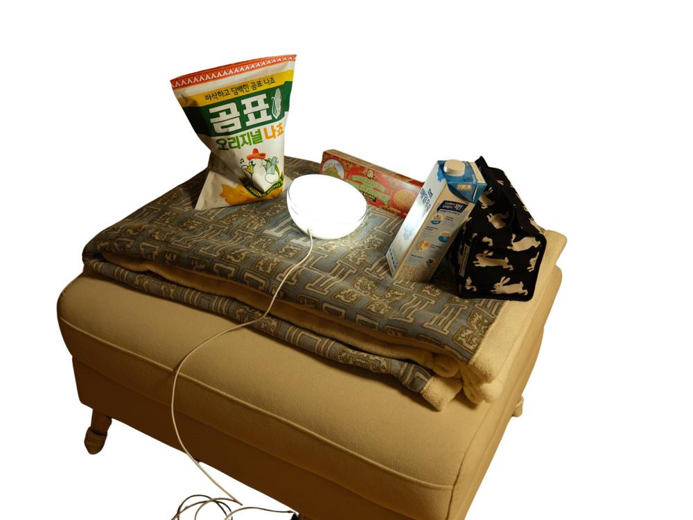
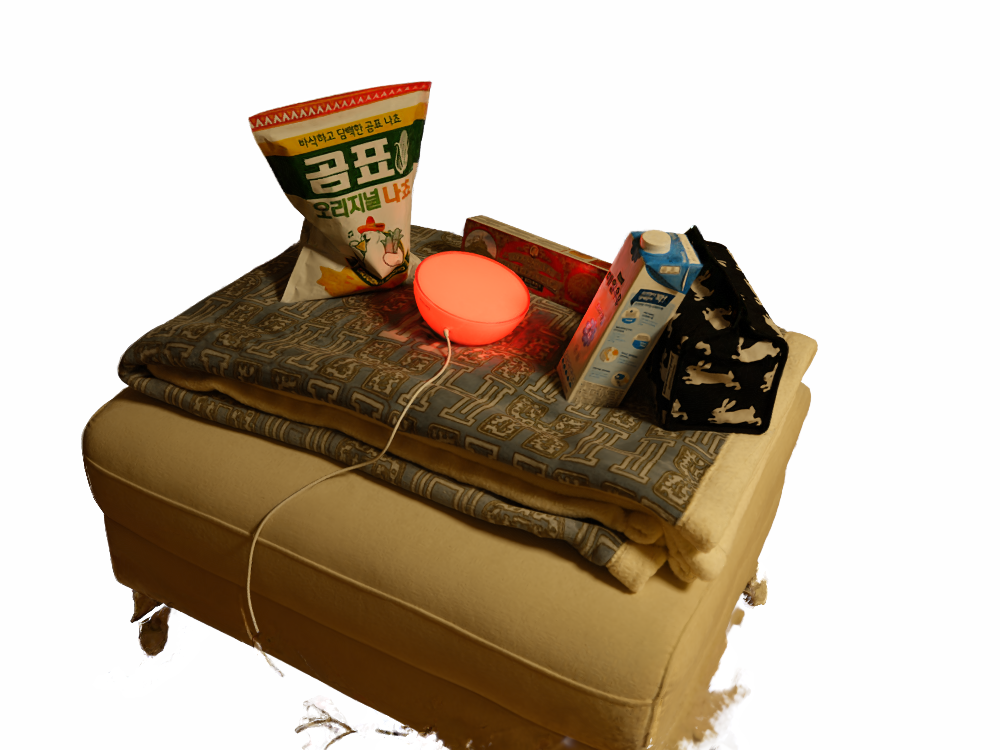
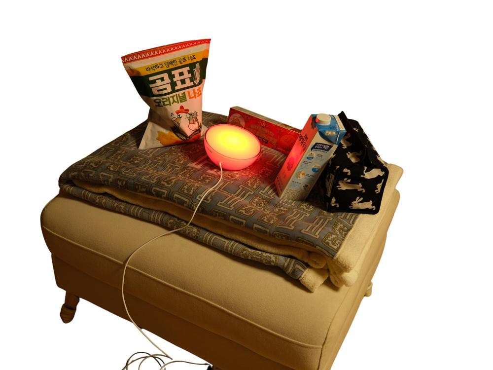
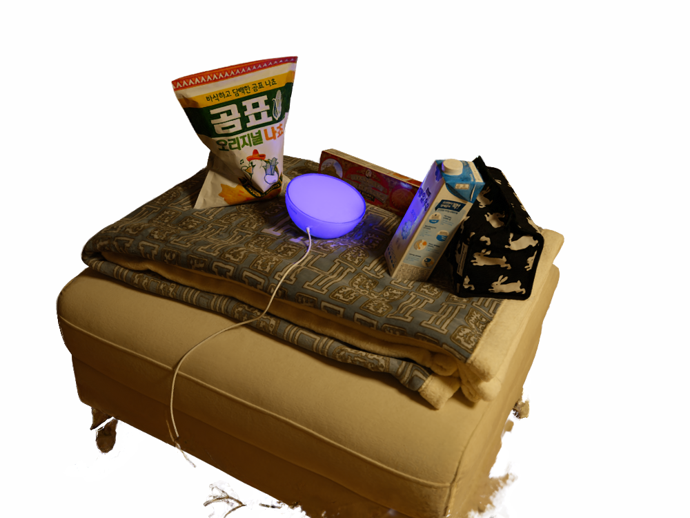
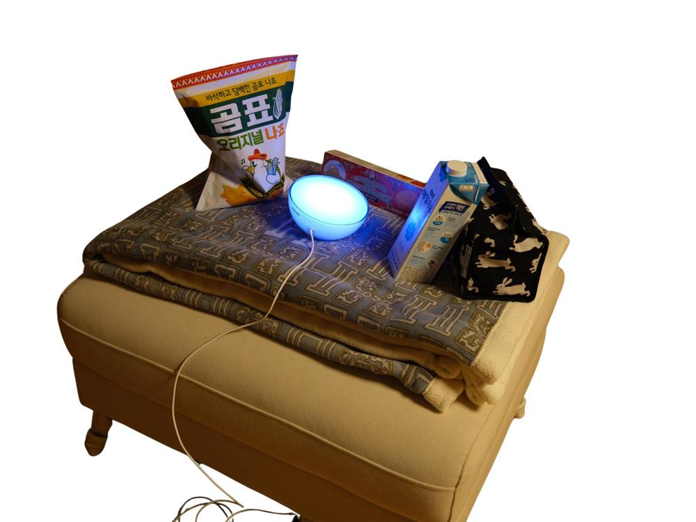
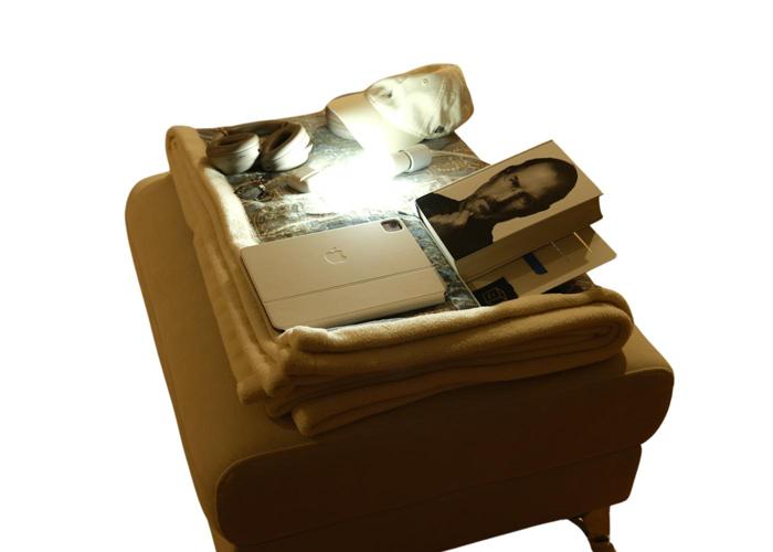
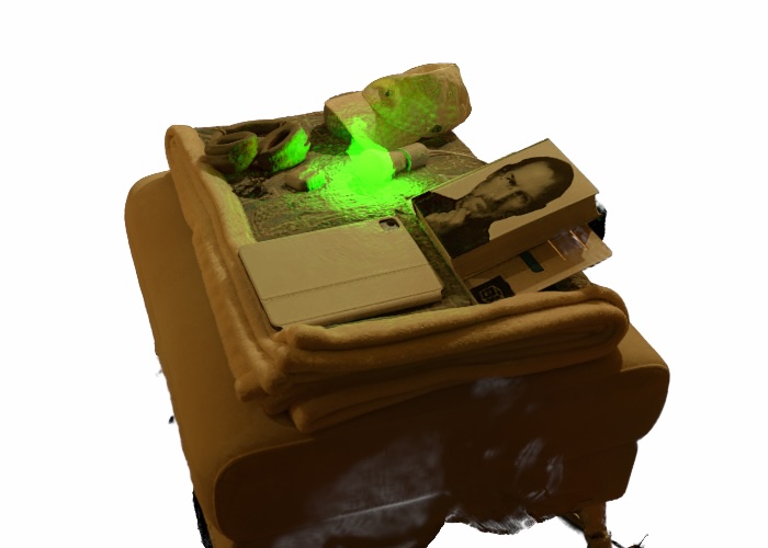
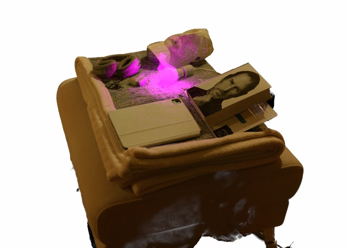
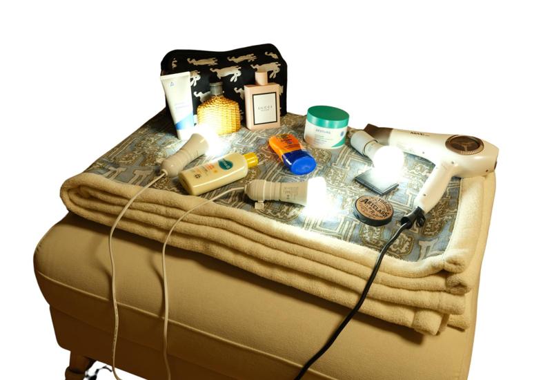
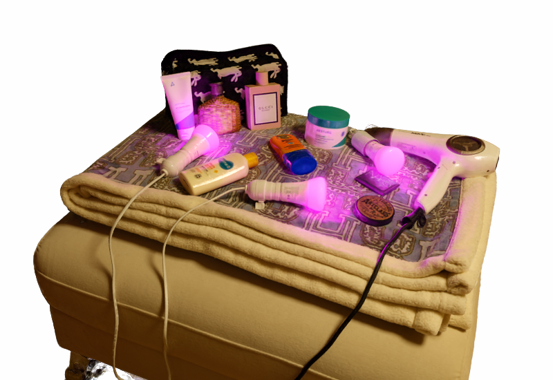
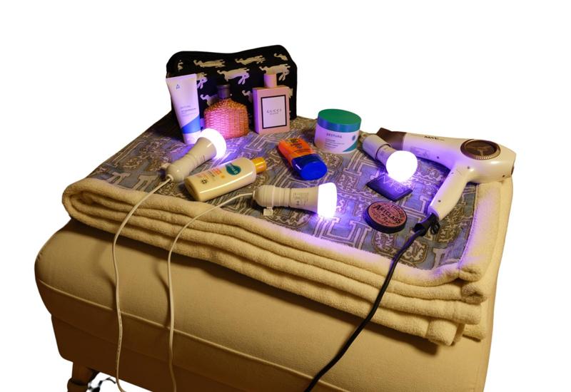
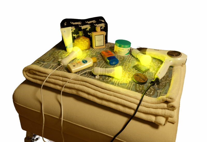
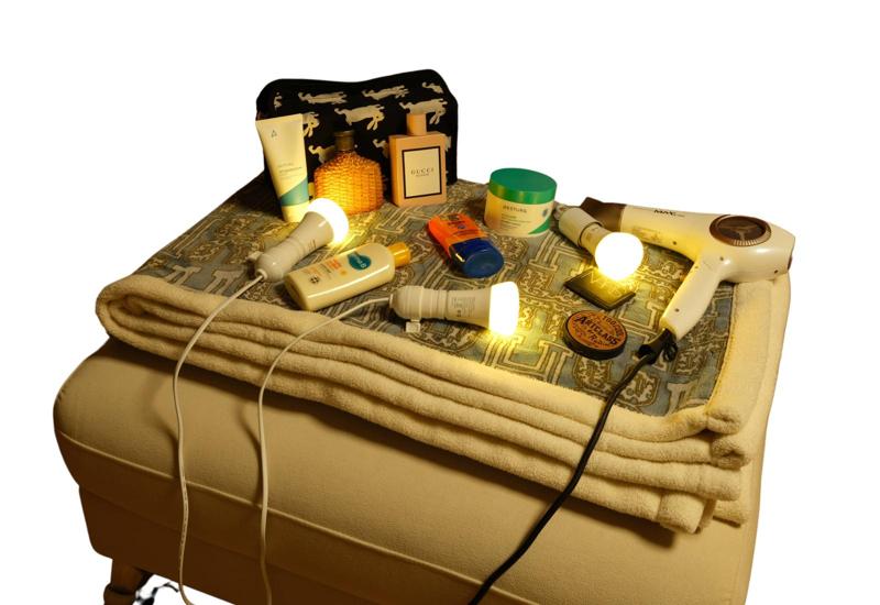
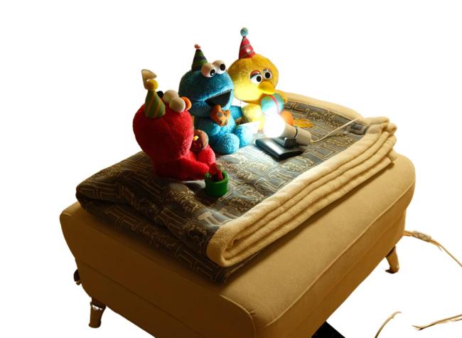
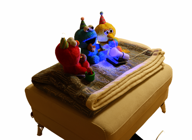
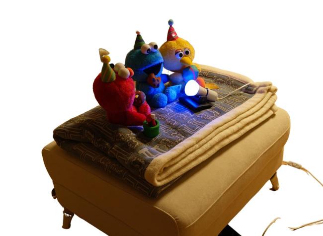
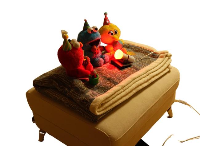
Figure 20: Qualitative results comparison with ground truth obtained using commercial smart bulbs.

	TensoIR	NeILF++	ESR-NeRF	TensoIR	NeILF++	ESR-NeRF
Emission
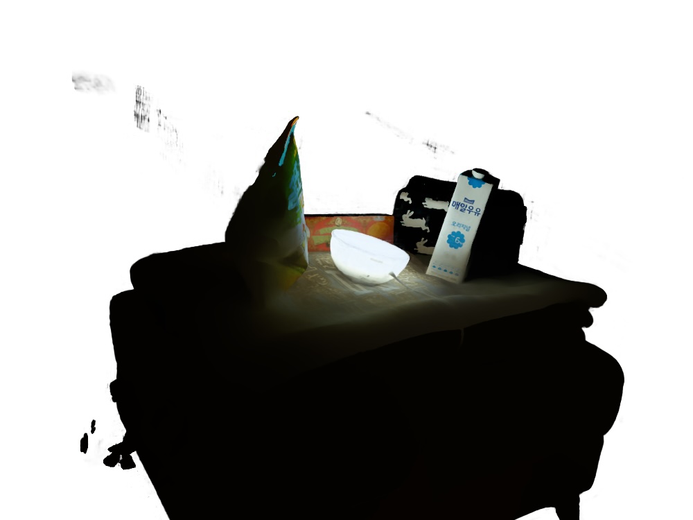
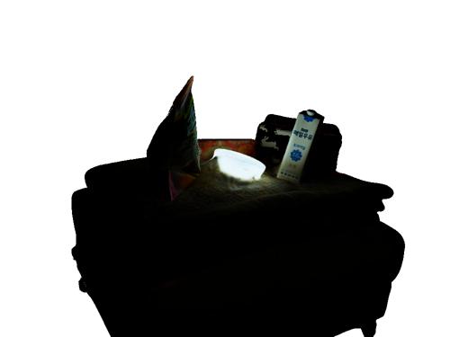
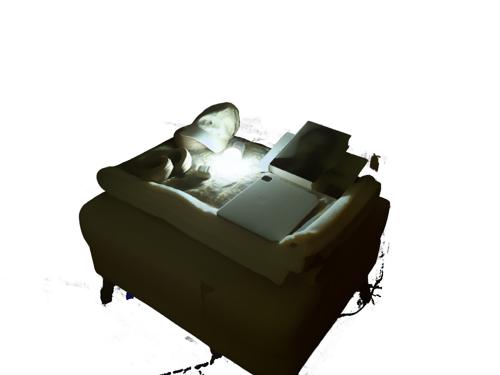
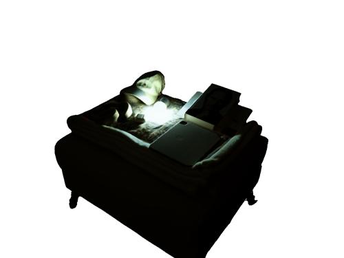
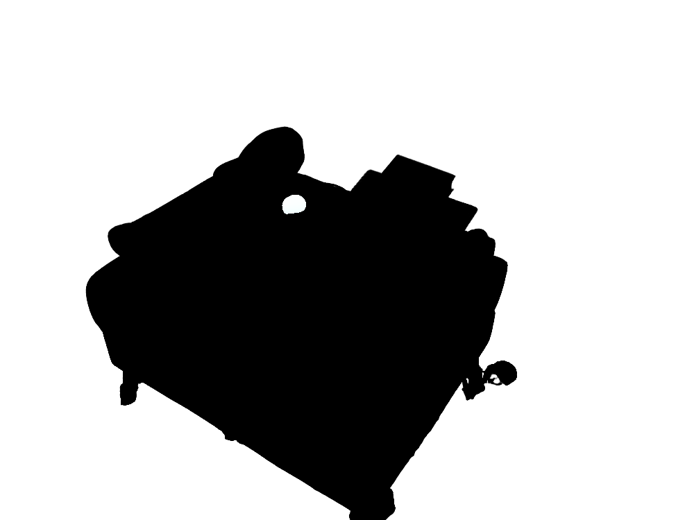
Albedo
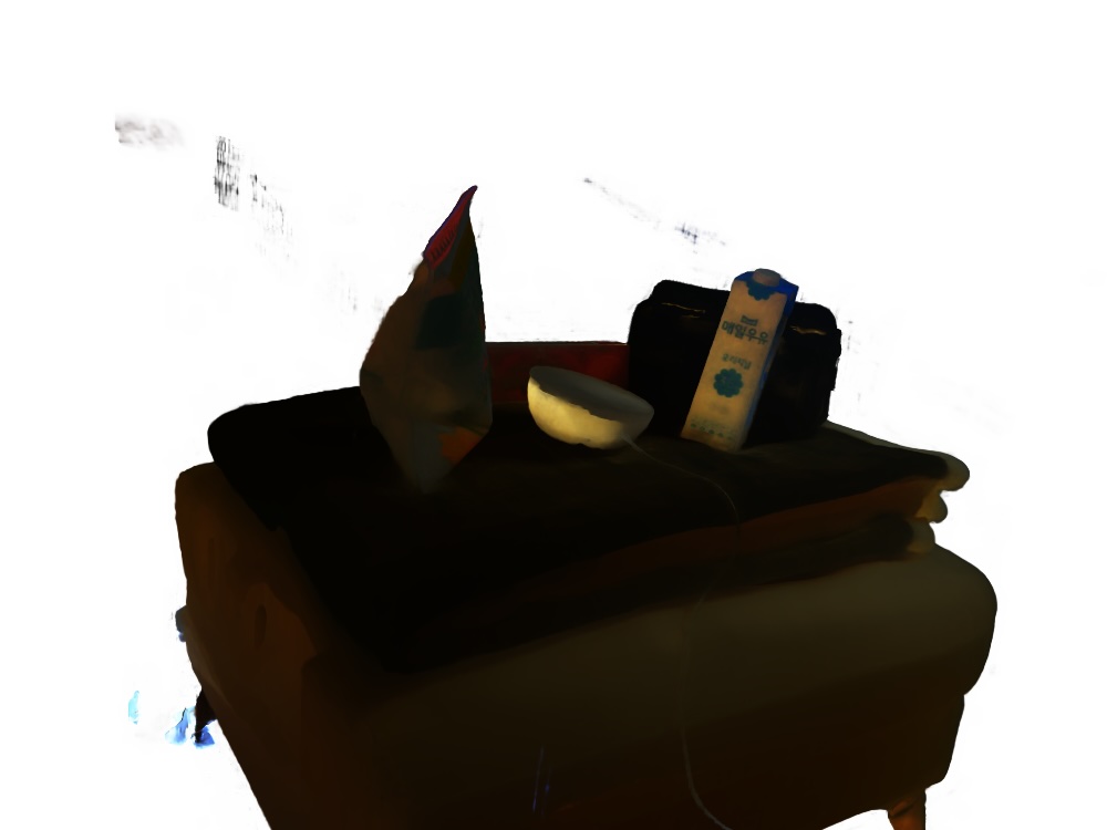
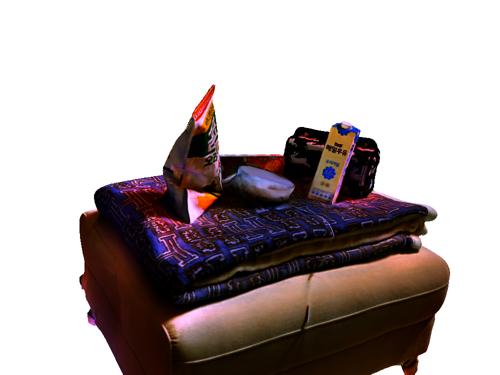
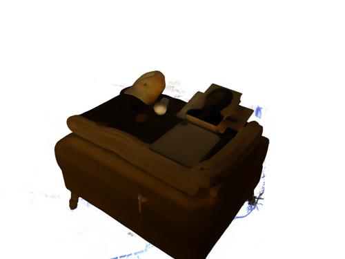
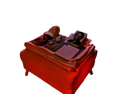
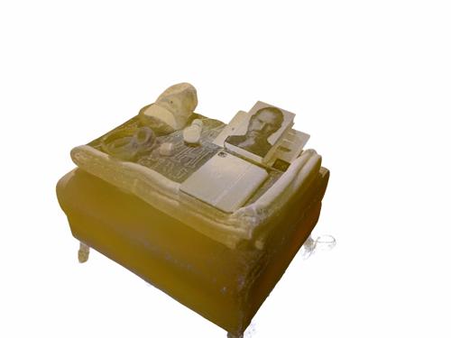
Roughness

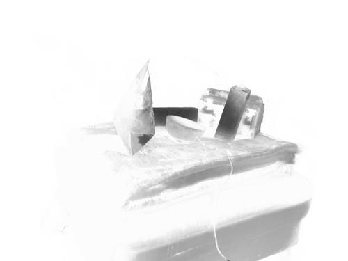
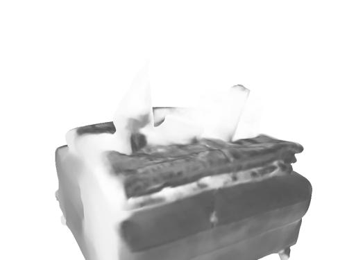
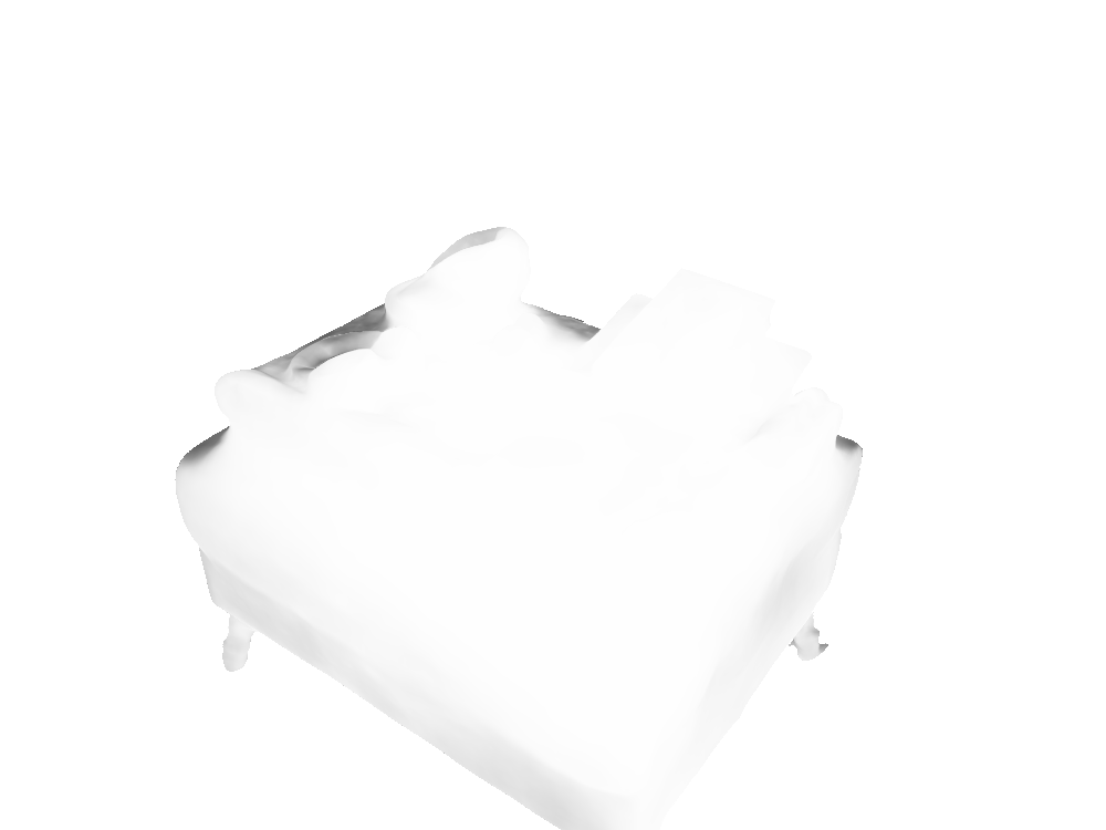
Figure 21: Comparison of identified emissive sources and decomposed BRDF.

	TensoIR	NeILF++	ESR-NeRF	TensoIR	NeILF++	ESR-NeRF
Emission
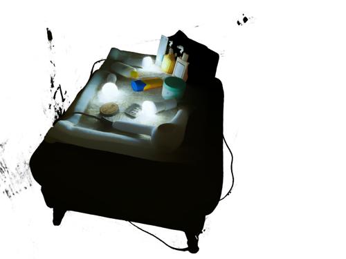
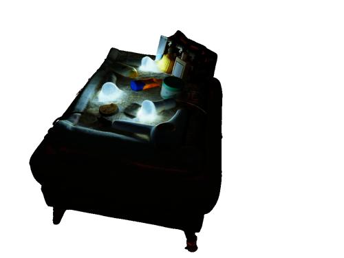
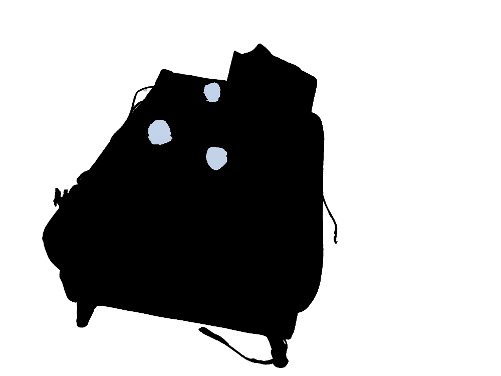
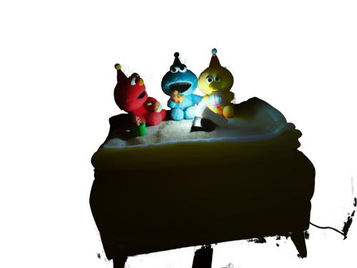
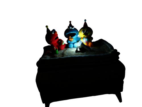
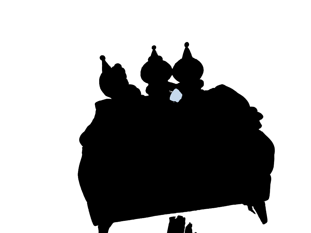
Albedo
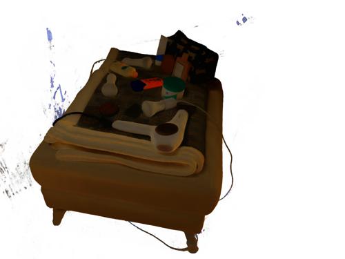
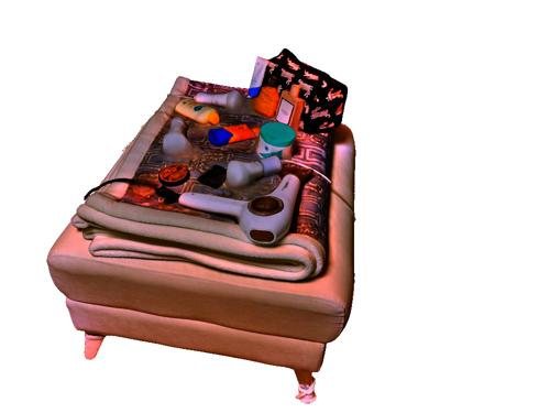
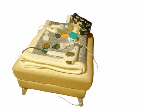
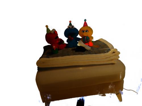
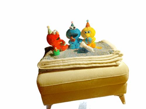
Roughness

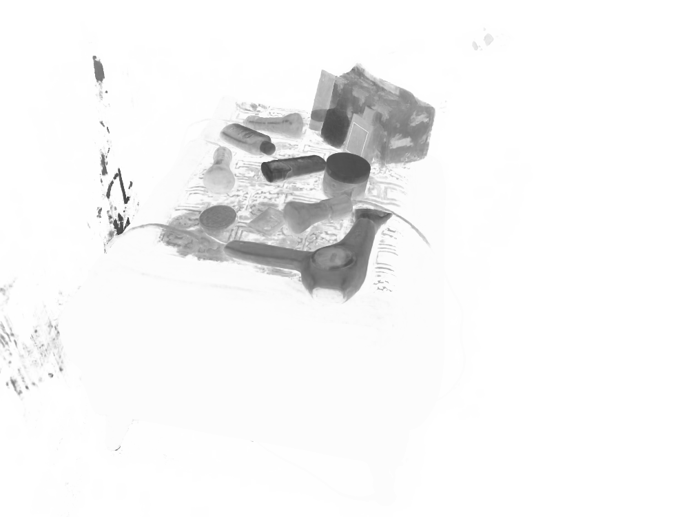
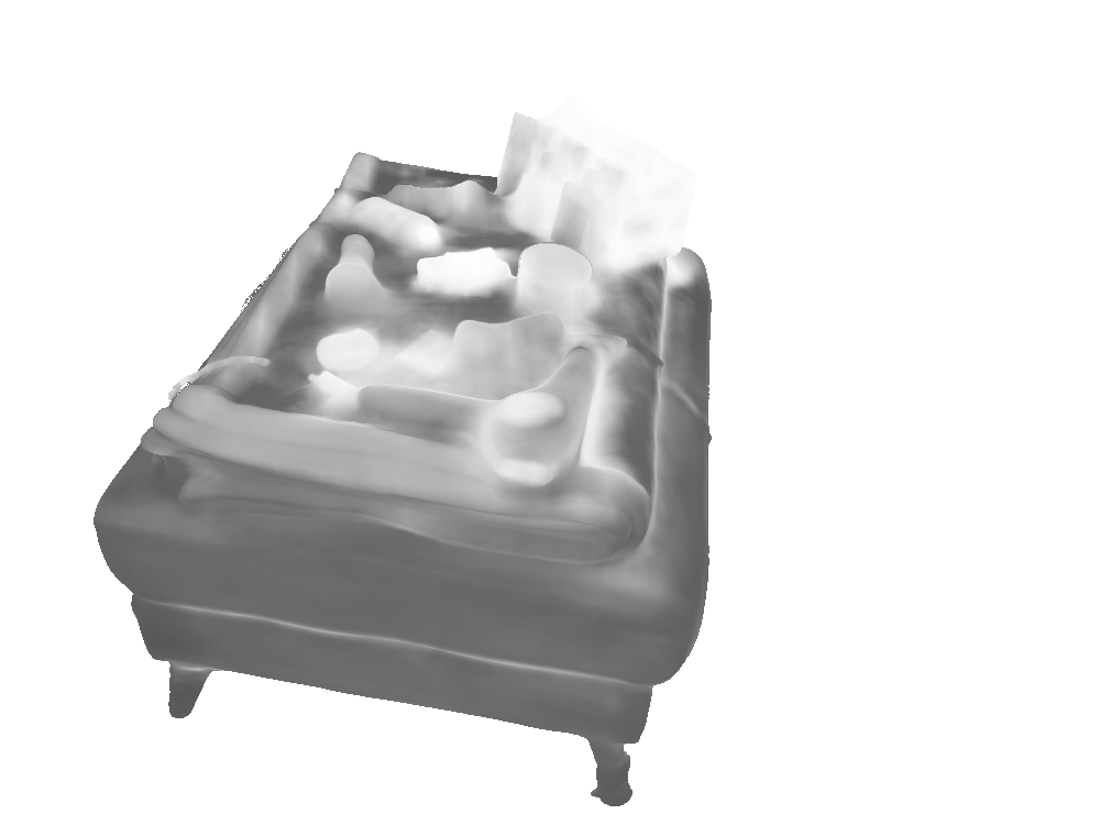
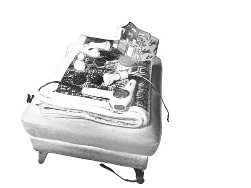
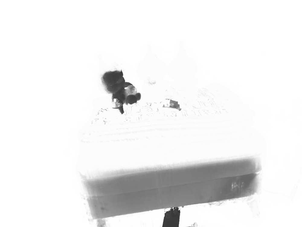
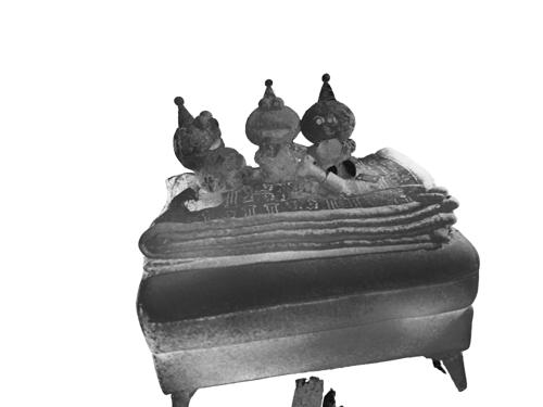
Figure 22: Comparison of identified emissive sources and decomposed BRDF.

8.3 Baseline Implementation

In our evaluation, we compared against two leading re-lighting methods, TensoIR [25] and NeILF++ [93], known for their ability to operate without prior knowledge of scene components Additionally, we made Twins, a method focused on emissive source reconstruction without relying on inverse rendering techniques. For an in-depth analysis of scene editing capabilities, we include PaletteNeRF [28], which achieves scene modification through re-colorization, and NeRF-W [38], which adjusts scene illumination by interpolating between learned latent vectors. For surface reconstruction evaluations on the DTU dataset, we selected state-of-the-art methods such as Voxurf [83] and NeuS [71], alongside Neural-PBIR [59], which offers a joint reconstruction of surfaces, materials, and environment maps. We utilized the official implementations provided by the authors for all baselines, with the exception of NeRF-W. We used the official implementation codes provided by the authors for all baseline methods except for Twins and NeRF-W. Twins employs a dual-model strategy for ’light-on’ and ’light-off’ conditions, using radiance differences for emissive source identification and scene illumination editing. NeRF-W leverages two latent embeddings for similar purposes, focusing on intensity adjustments. Both Twins and NeRF-W are based on the Voxurf architecture to ensure a fair comparison with ESR-NeRF. For NeILF++, we omitted the use of prior scene information to align with methods that do not use geometry hints like object meshes or oriented point clouds. Neural-PBIR was excluded from emissive source reconstruction experiments as the code is not publicly available yet. Baseline performance data on the DTU dataset are borrowed directly from the Voxurf, NeuS, and Neural-PBIR papers.

8.4 Real Scene

We showcase the effectiveness of ESR-NeRF in identifying emissive sources in real-world scenes. Camera poses are estimated using COLMAP [51]. We use commercial smart light bulbs from Philips, which offer control over light colors. Since precise control over the color of the smart bulbs is infeasible, we provide qualitative results for emissive source identification and scene editing in real scenes. Fig. 18 presents the decomposed scene components, such as normal, base color, roughness, metallic, and the environment map. In Fig. 19, our method successfully identifies emissive sources, enabling scene illumination adjustments. Fig. 20 presents qualitative results for comparison with ground truth data. Although our model successfully identifies emissive sources, it encounters difficulties with complex reflections inside light bulbs, as indicated by the bright spots at the bulb centers in the ground truth edit images. Despite these challenges, ESR-NeRF stands out as the first NeRF-based inverse rendering method to address the reconstruction of emissive sources, enabling scene illumination modifications through the identification of light sources within a scene.

8.5 Reconstructed Scene Components

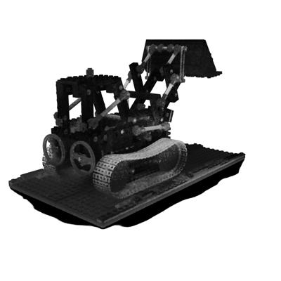
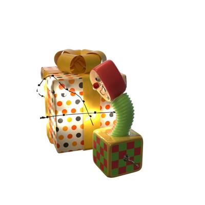
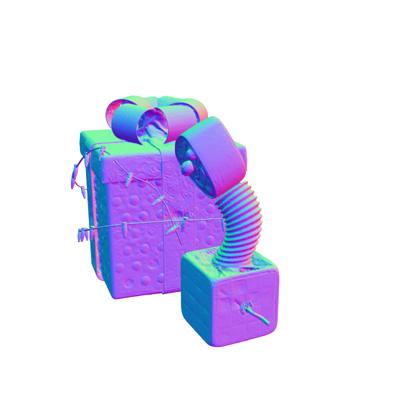
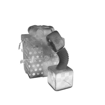
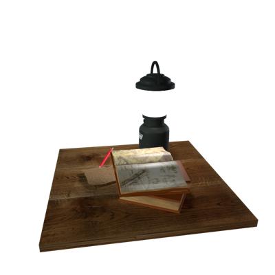
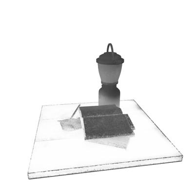
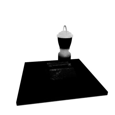
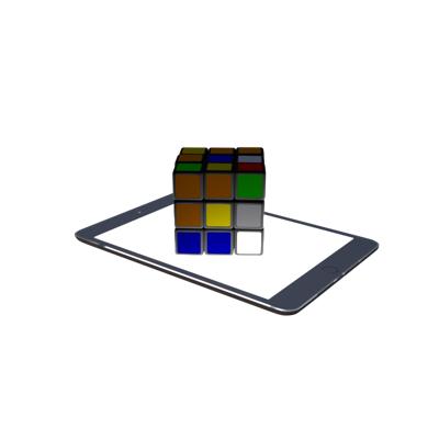
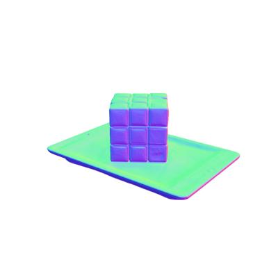
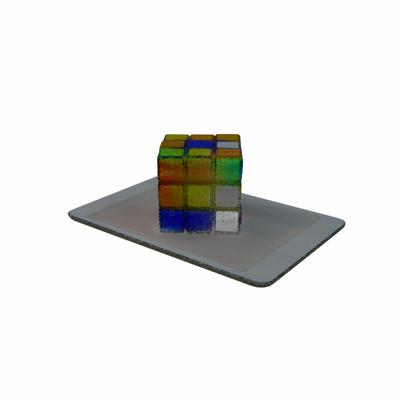
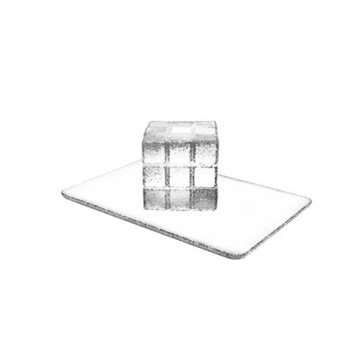
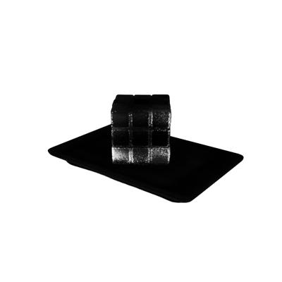
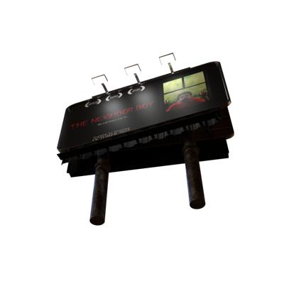
Figure 24: Decomposed scene components on scenes with white-colored emissive sources.

	TensoIR	NeILF++	ESR-NeRF	TensoIR	NeILF++	ESR-NeRF
Emission
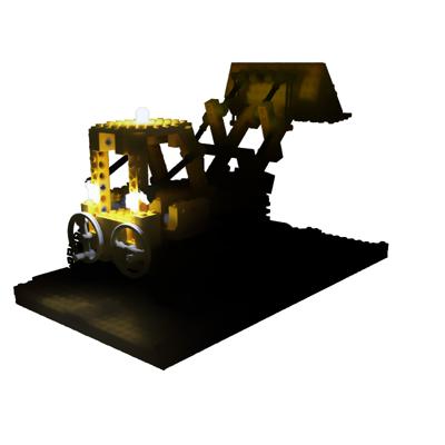
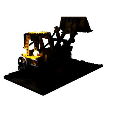
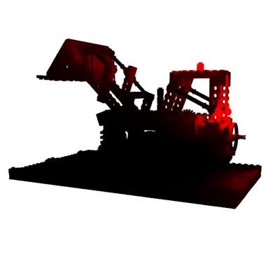
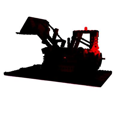
Albedo
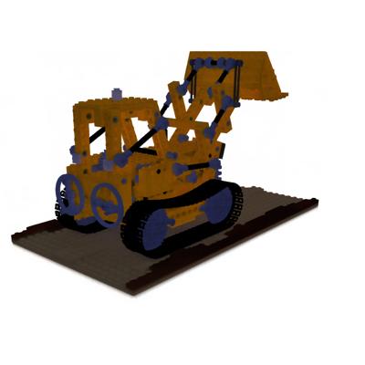
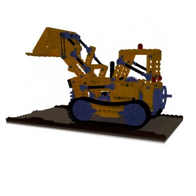
Roughness

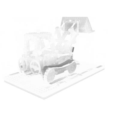
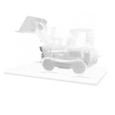
Figure 26: Comparison of identified emissive sources and decomposed BRDF on the Lego scene. Left: Lego white. Right: Lego vivid.

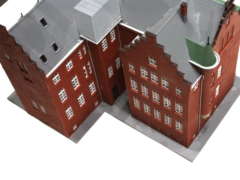
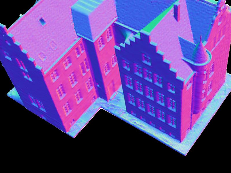
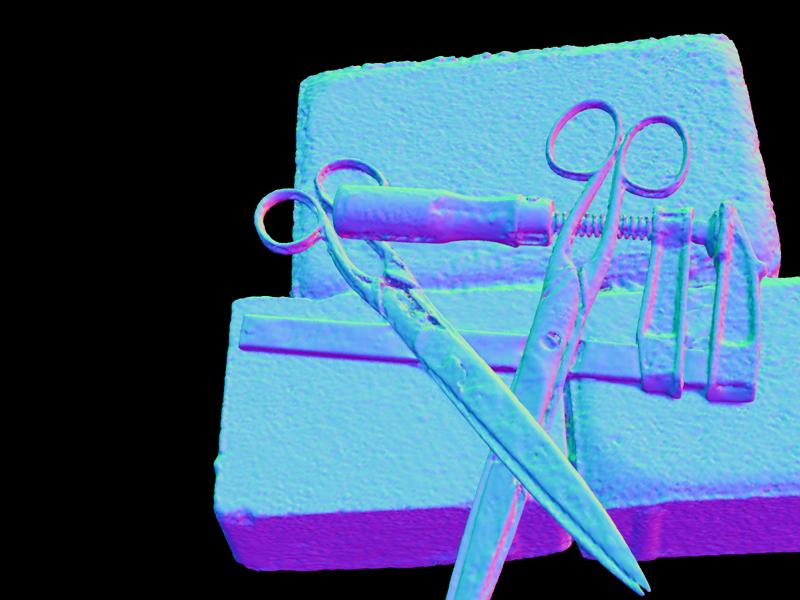
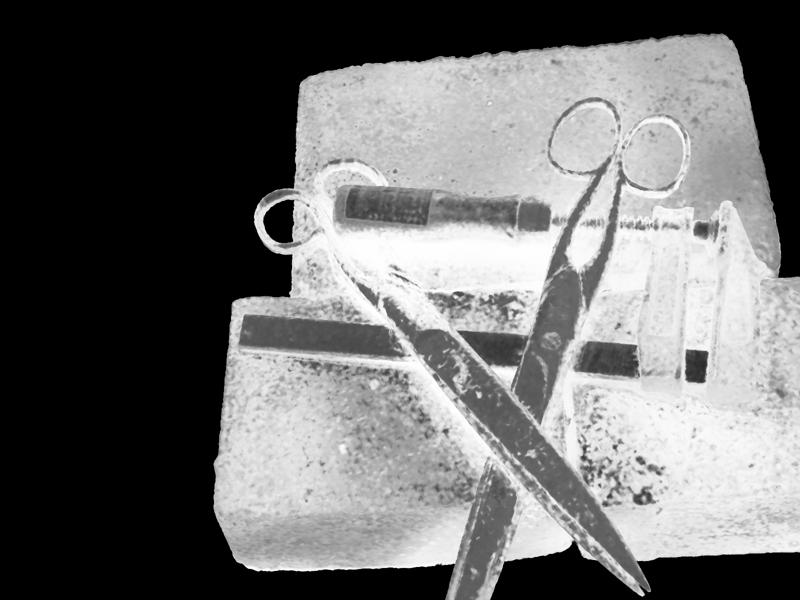
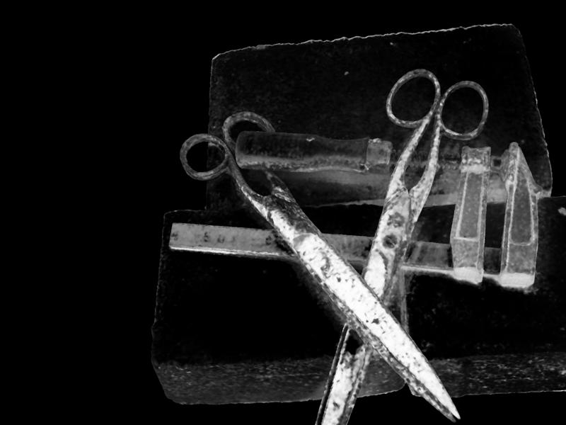
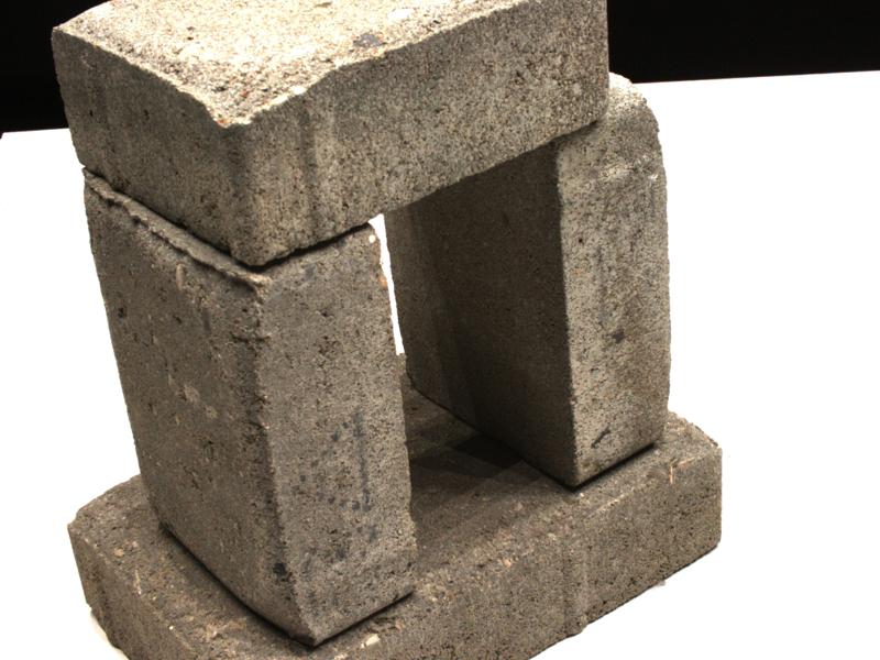
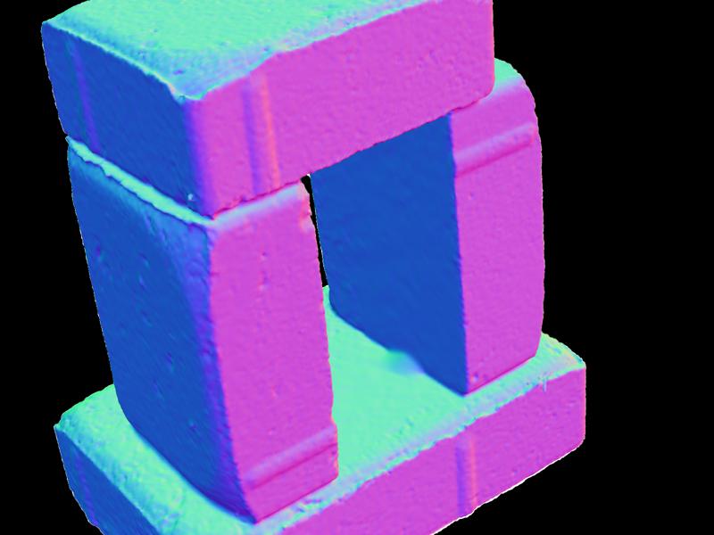
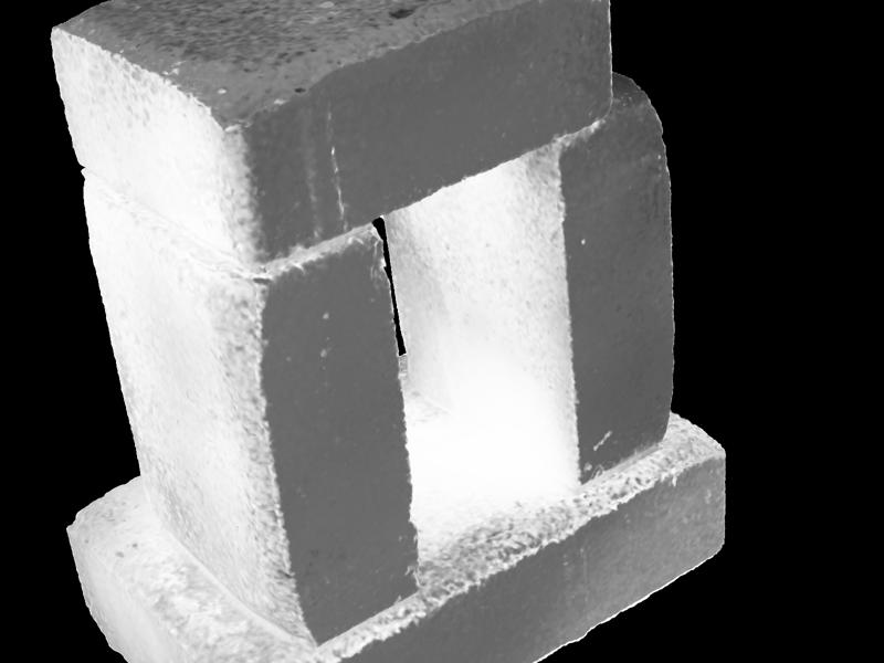
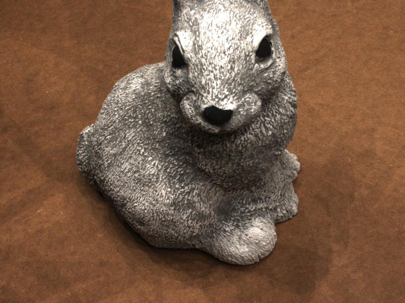
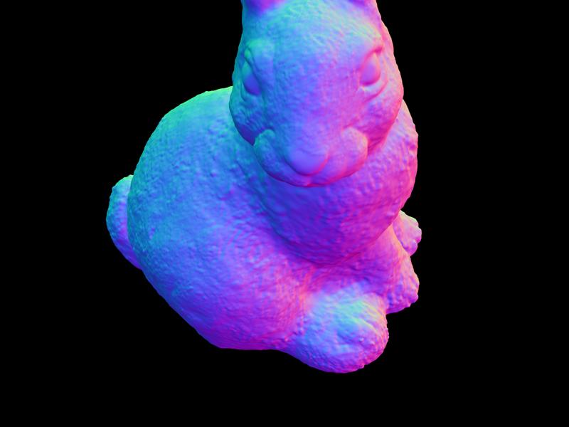
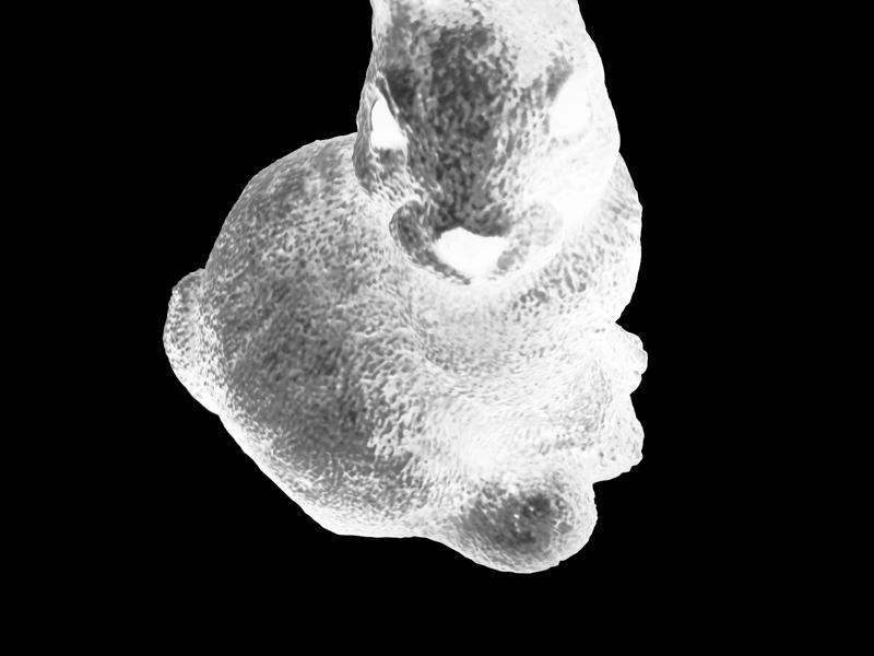
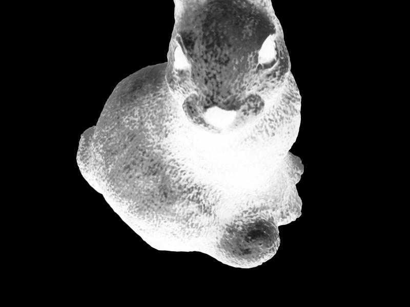
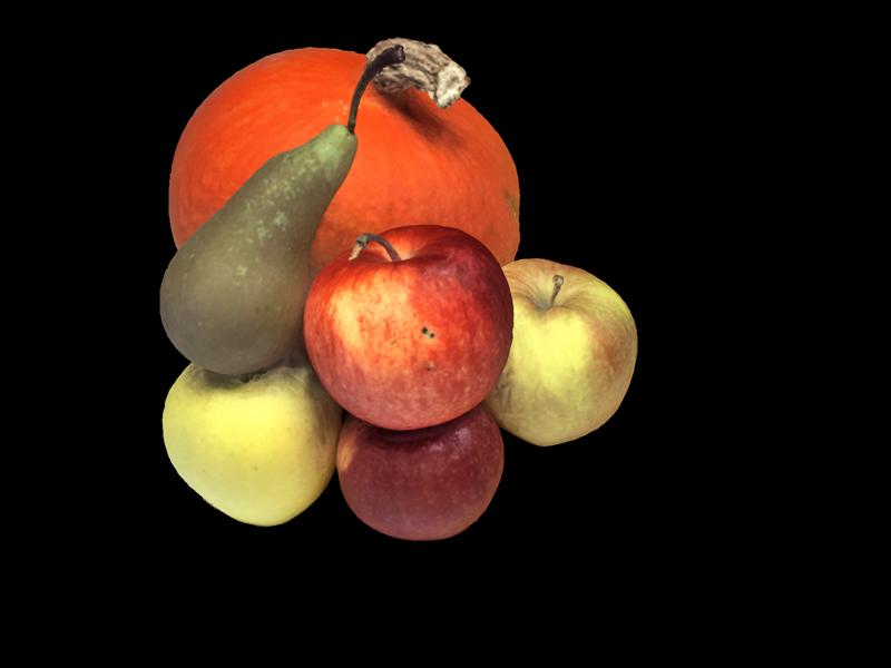
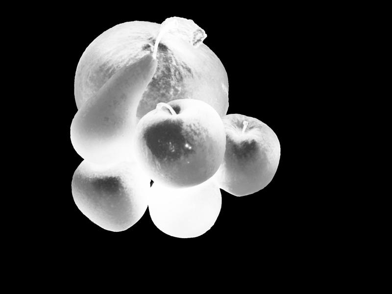
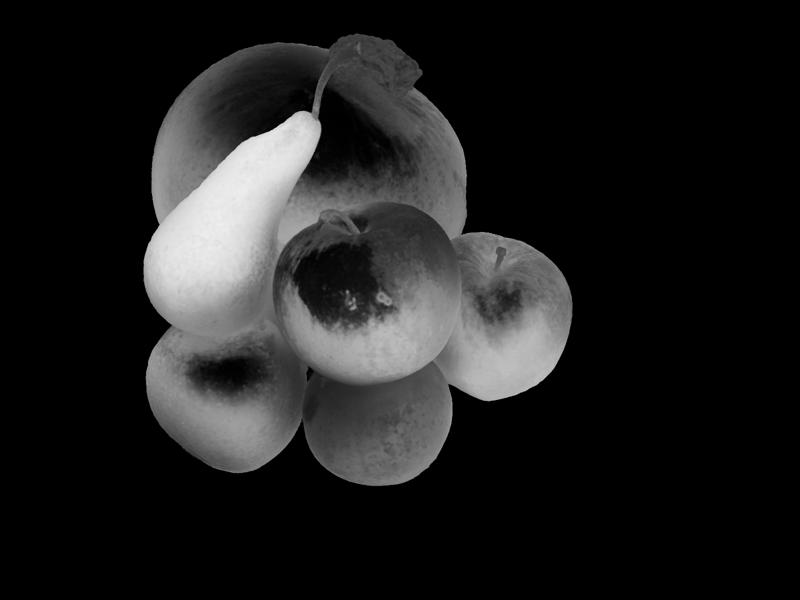
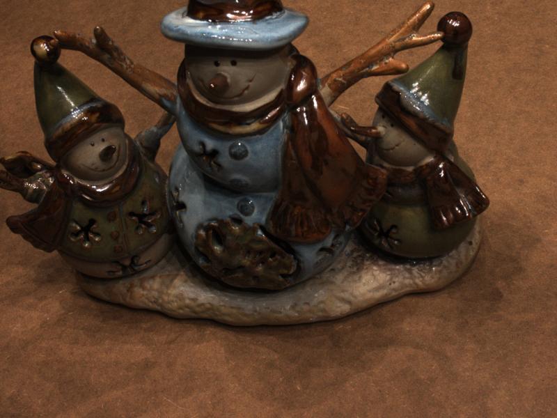
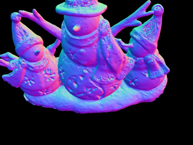
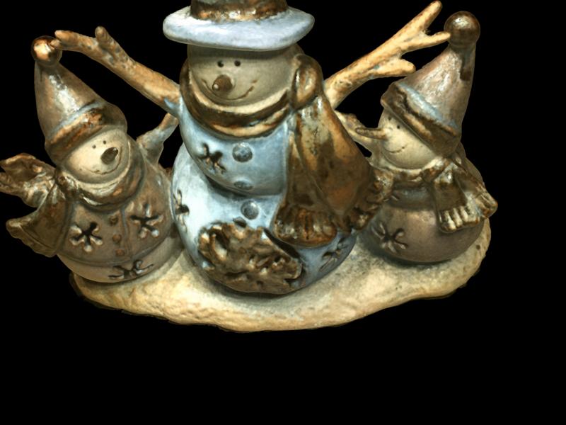
Figure 31: Decomposed scene components on DTU scenes without emissive sources.

We present the reconstructed components of our synthetic scenes, including emissions, surface normals, and BRDF, in Fig. 24 and 25. We also provide the comparison of the reconstructed emission and BRDF performance among TensoIR, NeILF++, and ESR-NeRF in Fig. 21 and 22 for real scenes and Fig. 26 to 30 for synthetic scenes. TensoIR and NeILF++ encounter difficulties, as does ESR-NeRF, in capturing precise roughness, often resulting in shadows being baked into the albedo. This issue is exacerbated by a relatively dark environment map, in contrast to previous works, and is compounded by strong emissions and shadows. Nevertheless, while BRDF results are comparable, ESR-NeRF distinguishes itself in its primary goal: the accurate reconstruction of emissive sources We also provide the reconstructed scene components on DTU dataset in Fig. 31 and 32.

	White colored												Vivid colored
	Lego		Gift		Book		Cube		Billboard		Balls		Lego		Gift		Book		Cube		Billboard		Balls
	IoU	MSE	IoU	MSE	IoU	MSE	IoU	MSE	IoU	MSE	IoU	MSE	IoU	MSE	IoU	MSE	IoU	MSE	IoU	MSE	IoU	MSE	IoU	MSE
w/o progressive	0.09	18.87	0.05	5.93	0.38	2.84	0.82	30.82	0.14	1.00	0.93	0.04	0.09	6.71	0.05	3.89	0.37	1.69	0.84	10.60	0.14	0.64	0.94	0.02
w/o sg	0.79	8.33	0.50	5.32	0.35	2.91	0.96	21.28	0.72	0.80	0.95	0.04	0.16	6.43	0.35	3.60	0.35	1.87	0.93	8.65	0.89	0.25	0.92	0.03
ESR-NeRF	0.81	8.38	0.60	3.49	0.96	1.19	0.97	17.87	0.84	0.46	0.95	0.04	0.51	5.48	0.59	2.50	0.96	0.51	0.97	7.94	0.88	0.26	0.94	0.03

Table 7: Per-scene metrics on emissive source reconstruction tasks. The IoU measures the source area identification (a higher value is better), and the MSE quantifies the difference between reconstructed images and HDR ground truth images (a lower value is better).

8.6 Illumination Decomposition

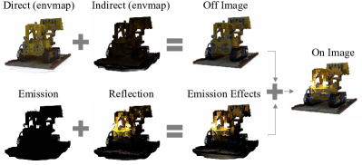
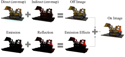
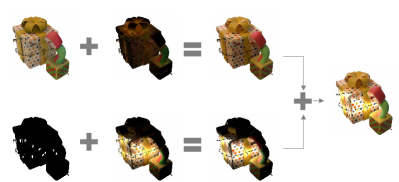
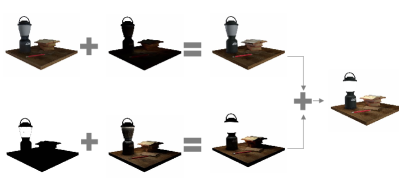
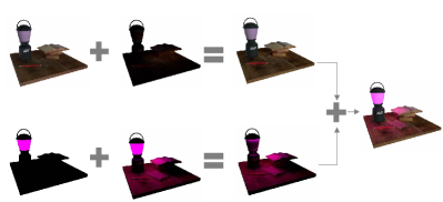
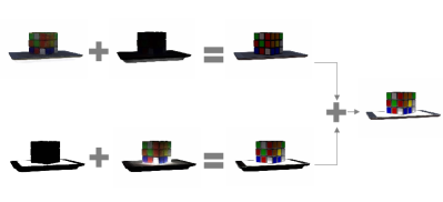
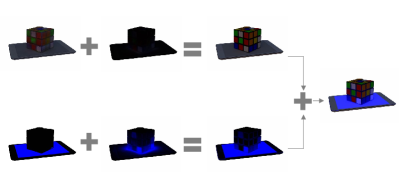
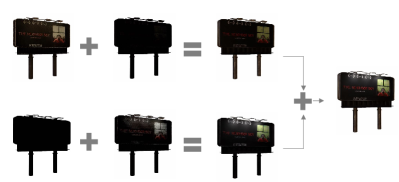
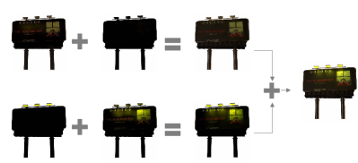
Figure 33: Illumination decomposition results. Left: scenes with white-colored, Right: scenes with vivid-colored emissive sources.

We present additional results of decomposed illumination in Fig. 33. These visualizations offer insights into the effectiveness of ESR-NeRF in factorizing the scene illumination. The off image, for instance, is generated by merging direct and indirect illumination from the environment map, as shown in the first row. The second row illustrates the decomposition of emission effects, including both the emission and its reflection. Light-on images are created by adding the light-off and the emission effects images.

8.7 Scene Editing w&w/o Radiance Fine-tuning

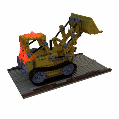
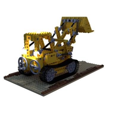
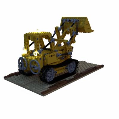
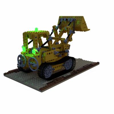
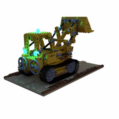
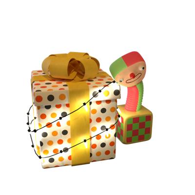
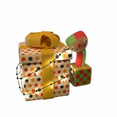
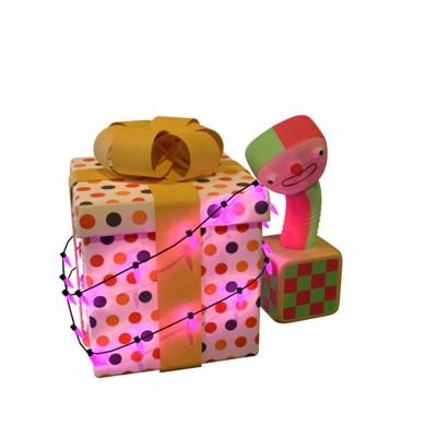
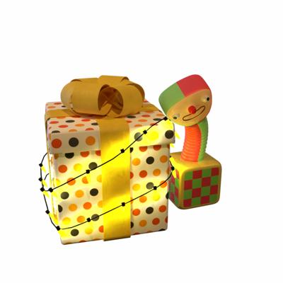
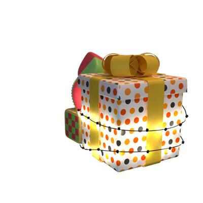
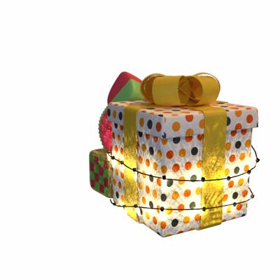
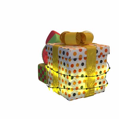
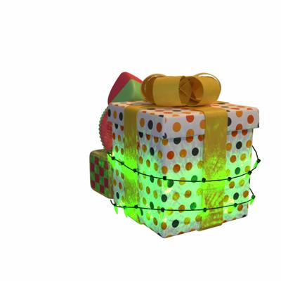
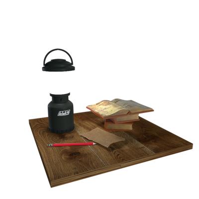
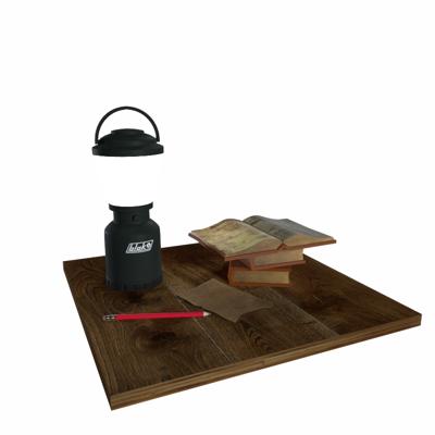
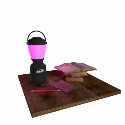
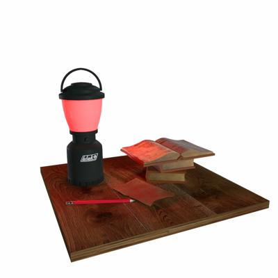
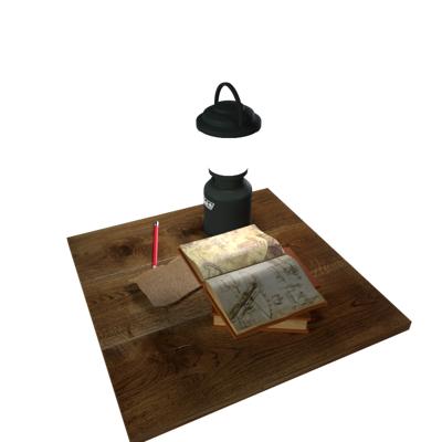
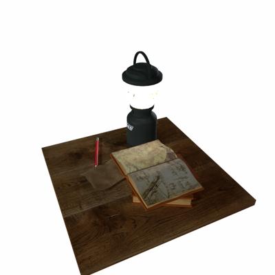
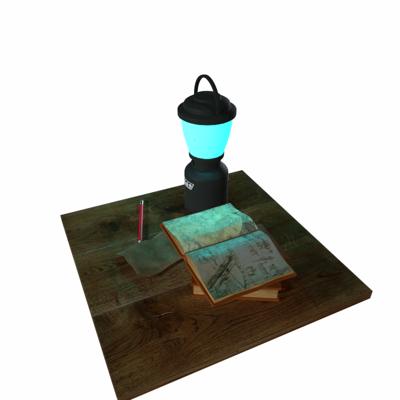
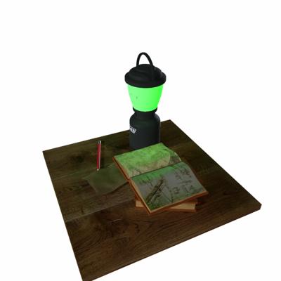
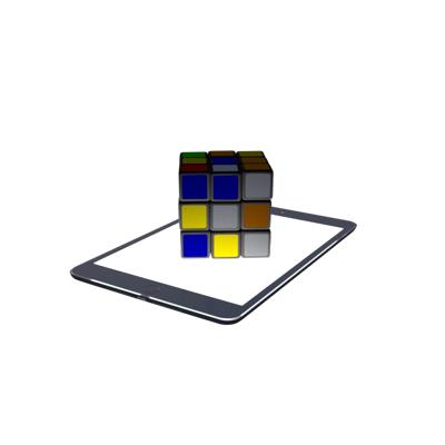
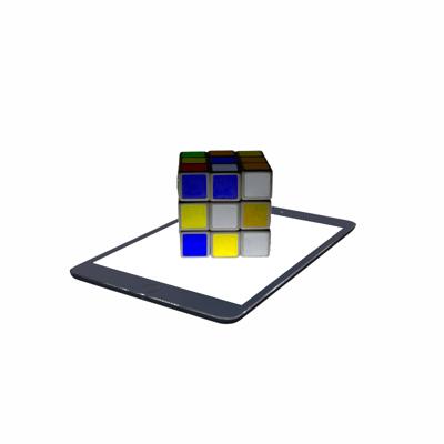
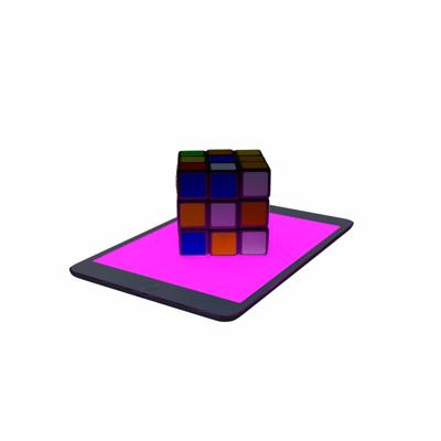
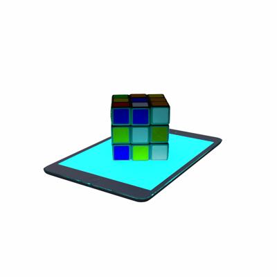
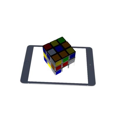
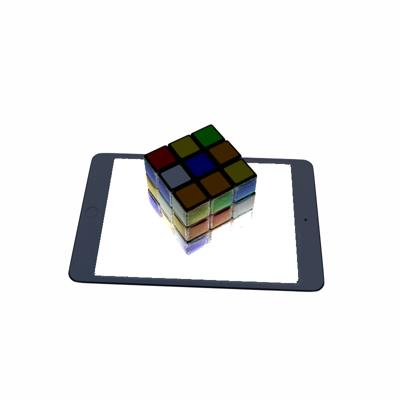
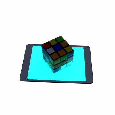
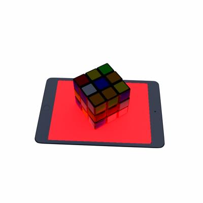
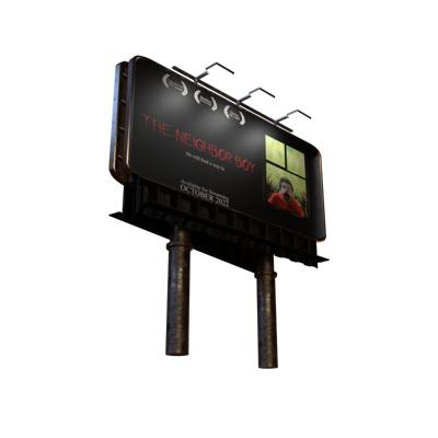
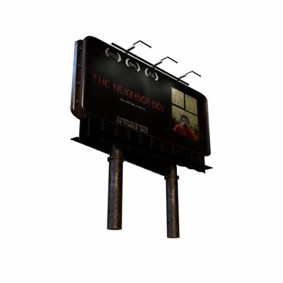
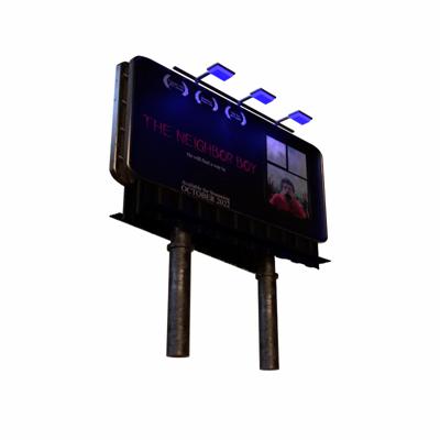
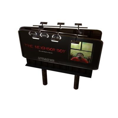
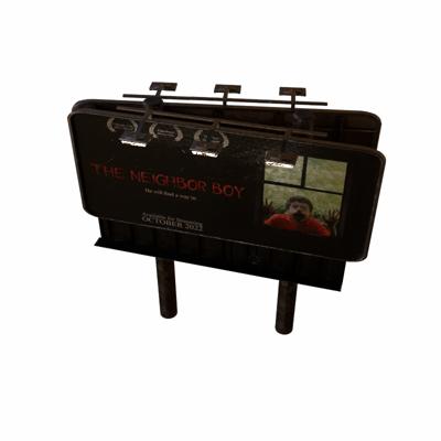
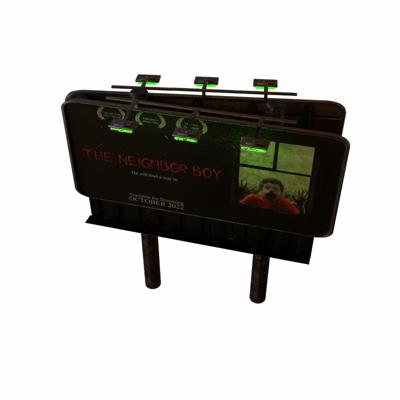
Figure 34: Re-lighting scenes containing white emissive sources. Left: through fine-tuning radiance fields, Right: computing direct illumination from reconstructed emissive sources.

Fig. 34 and 35 present additional scene editing examples, illustrating various scenarios including intensity and color edits, as well as their combination. As discussed in the conclusion section of the main paper, scene illumination can be adjusted without fine-tuning radiance fields, using alternative methods. Results on the right side of Fig. 34 to 35 are rendered by calculating only direct illumination from emissive sources for re-lighting, a technique commonly used in prior research [25, 99, 98], bypassing the fine-tuning of trained networks. This approach is particularly effective for scenes with vividly colored emissive sources, as shown in Fig. 36. To evaluate the effectiveness of direct illumination in scene editing, we provide quantitative results for each scenario in Tab. 9 and 10. Quantitative comparisons for scenes with vivid-colored emissive sources are detailed in Tab. 11 and 12.

8.8 Analysis of Learnable Tone-mapper

We eliminate the constraint on the range of radiance values to address the unbounded nature of emissive sources and their reflections. Instead of the commonly used sigmoid activation function in NeRF-based methods [40, 55, 12, 99, 101] for radiance prediction, we employ the softplus activation, extending the radiance range from $[0,1]$ to $[0,\infty]$.

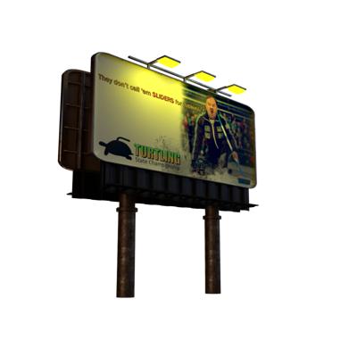
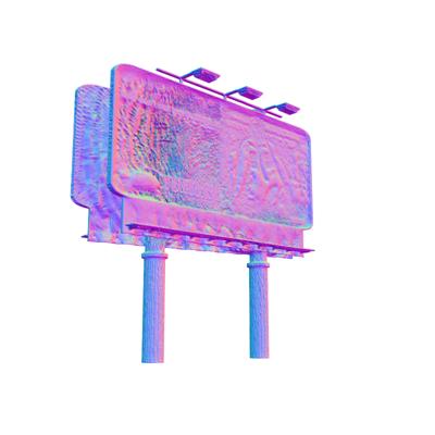
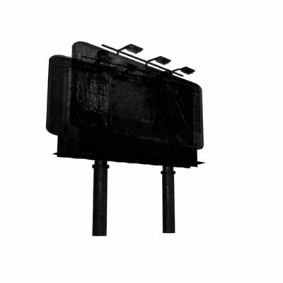
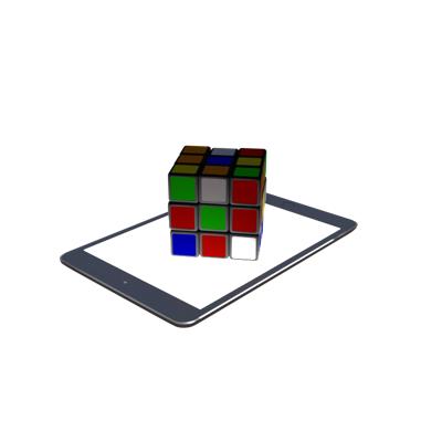
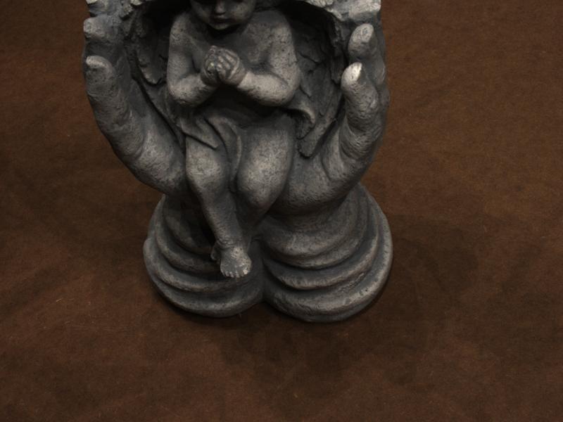
Figure 39: Erroneously reconstructed surfaces and rendered linear images when using softplus activation for radiances without utilizing the tone-mapper $m_{\theta}$. Gamma correction is applied to linear images for easy comparison.

However, this modification may lead to inaccurate surface reconstructions, as highlighted in the main paper. Fig. 39 shows instances where surfaces become semi-transparen, lose structural details, and the rendered images significantly deviate from the ground truth, making the accurate reconstruction of emissive sources infeasible.

Image	$\lambda_{\tau}=0.001$	$\lambda_{\tau}=0.01$	$\lambda_{\tau}=0.1$	$\lambda_{\tau}=1.0$
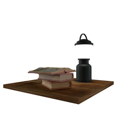
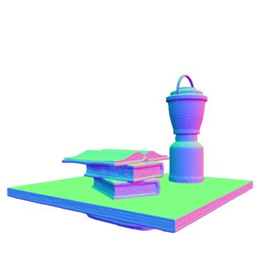
					Normal
					Rendered
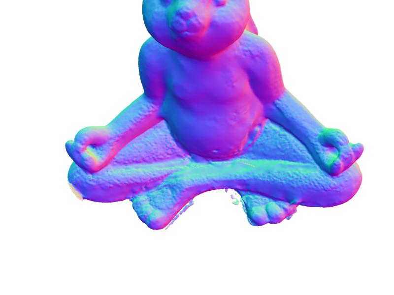
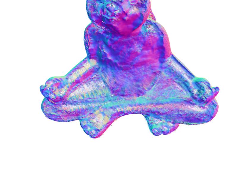
					Normal
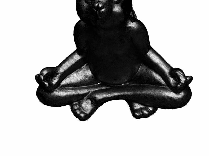
					Rendered

Figure 37: Reconstructed surface normals and rendered linear images with varying $\lambda_{\tau}$ values. Gamma correction is applied to linear images for easy comparison.

To address this issue, we introduce a learnable tone-mapper $m_{\theta}$, taking positionally encoded HDR linear color as input and produce LDR sRGB colors outputs. Fig. 37 reveals that this tone-mapper helps in obtaining accurate surface normals and rendering photo-realistic images. Nonetheless, a trade-off exists between the quality of surface normals and rendered images, when using the learnable tone-mapper. For example, a low $\lambda_{\tau}$ value, which indicates a heavier reliance on the tone-mapper in the rendering loss, may improve surface details but linear color values deviate significantly from expectations. This discrepancy occurs as the correlation between predicted linear colors and actual image pixel colors weakens with lower $\lambda_{\tau}$ values. Conversely, a higher $\lambda_{\tau}$ compromises surface reconstruction quality. Thus, setting $\lambda_{\tau}$ requires careful consideration of the balance between surface detail and color accuracy.

Interestingly, the choice of $\lambda_{\tau}$ also impacts the reconstruction of emissive sources in real scenes. A high $\lambda_{\tau}$ tends to result in lower intensity of reconstructed emissive sources. Re-lighting experiments in Fig. 23 show illumination effects confined to a narrow area compared to ground truth data. We suspect the camera may edit images for low contrast and apply color grading, particularly in HDR scenes. We used the Fuji 100s camera. A high $\lambda_{\tau}$ in the rendering loss could be problematic, as it aims to align gamma-corrected linear values with manipulated colors. Based on this insight, we slightly reduced $\lambda_{\tau}$ by 0.1 to enhance emission intensity (1.4 vs. 37.2) and expand reflections in re-lighting scenarios.

High $\lambda_{\tau}$	Low $\lambda_{\tau}$	Pseudo G.T.

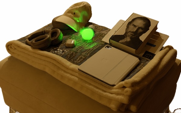
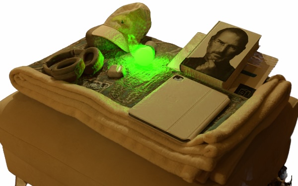
Figure 23: Scene edit results on jobs scene. Lower $\lambda_{\tau}$ results in stronger emission. The middle image is rendered with direct light for proving enhanced emission strength.

8.9 Near-zero IoU Results of Baselines

State-of-the-art re-lighting methods struggle with ambiguities surrounding emissive sources, often failing to accurately identify them. These methods typically cannot differentiate between reflections and emissions, leading to most regions being misclassified as emissive sources. This challenge is reflected in Tab. 8, where baseline methods exhibit near-zero IoU performance across various scenes. Despite extensive trinary grid searches with an interval of 0.01 for thresholding values to report the peak performance of baselines, ESR-NeRF consistently outperforms them. Additionally, our method’s efficacy in classifying rays into the uncertain group for emissive source identification highlights its superiority in this task. This is further supported by additional results obtained using thresholding techniques applied to the baselines.

	White colored						Vivid colored
	Lego	Gift	Book	Cube	Billboard	Balls	Lego	Gift	Book	Cube	Billboard	Balls
NeILF++	0.00	0.01	0.04	0.39	0.00	0.07	0.00	0.01	0.04	0.39	0.00	0.07
TensoIR	0.00	0.01	0.04	0.37	0.01	0.07	0.00	0.01	0.04	0.37	0.01	0.07
ESR-NeRF	0.81	0.60	0.96	0.97	0.84	0.95	0.51	0.59	0.96	0.97	0.88	0.94
NeILF++ ($*$)	0.43	0.07	0.95	0.93	0.01	0.91	0.30	0.09	0.95	0.94	0.02	0.92
TensoIR ($*$)	0.71	0.15	0.95	0.95	0.76	0.95	0.33	0.15	0.95	0.96	0.77	0.95
ESR-NeRF ($*$)	0.81	0.60	0.98	0.98	0.94	0.96	0.51	0.61	0.98	0.97	0.93	0.94

Table 8: Results of emissive source identification. The IoU measures the source area identification (a higher value is better). The asterisk (*) denotes that thresholding is applied to reconstructed emission strengths.

8.10 Failure Cases in Scene Editing

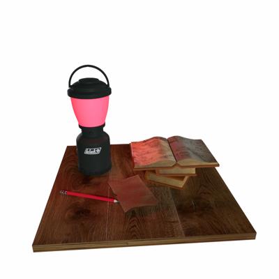
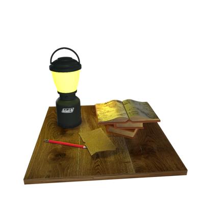
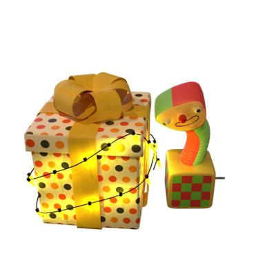
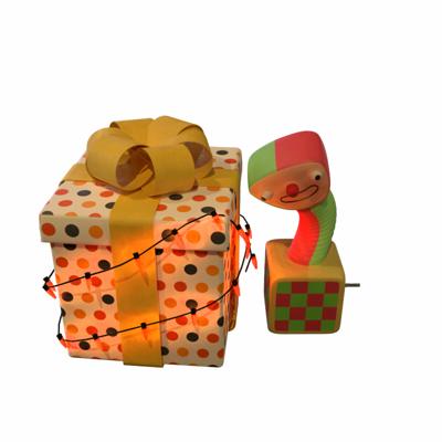
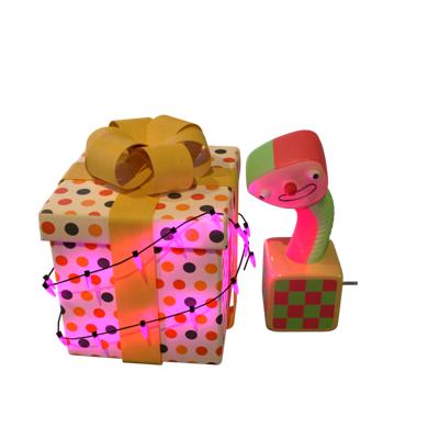
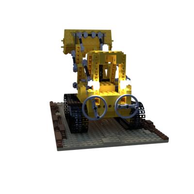
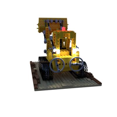
Figure 38: Failure cases for editing scene illumination using the radiance fine-tuning method.

We also present failure cases in scene editing, discussing the limitations of the radiance fine-tuning method for re-lighting in §4.5 of the main paper. While ESR-NeRF effectively reconstructs and manipulates emissive sources, the radiance fine-tuning method for re-lighting has its limitations. These are depicted in Fig. 38, where we note that LTS learning-based radiance fine-tuning may be constrained to color adjustments within the training spectrum. In other words, using the LTS loss to transfer radiance within light transport segments may be weak in representing new colors that traverse unobserved light paths during training. For example, it can shift colors from yellow to green but not to blue. Additionally, the network’s inherent smoothness capability may introduce illumination inaccuracies. In the last row in Fig. 38, changing only the top emissive source to red inadvertently affects the bulldozer’s lower ceiling.

Exploring alternative rendering approaches could address these issues. We showcase scene editing results by computing direct illumination from emissive sources in Fig. 36, enabling changes to any colors. Reconstructing emissive sources using ESR-NeRF, then extracting emission texture maps to use rendering engines like Blender [13] or Mitsuba [22] is also promising. Howver, the texture map extraction in NeRF-like methods often faces severe UV atlas fragmentation. Recent methods like Nuvo [56] offer some hope for feasible emission texture editing. We consider these avenues for future exploration

Image	Emissoin	Normal	Base Color	Roughness	Metallic

Image	Emissoin	Normal	Base Color	Roughness	Metallic

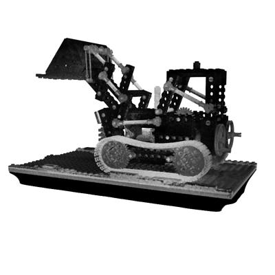
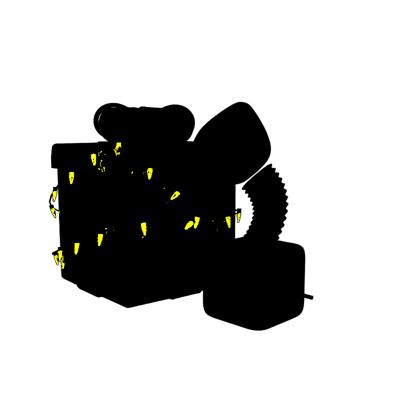
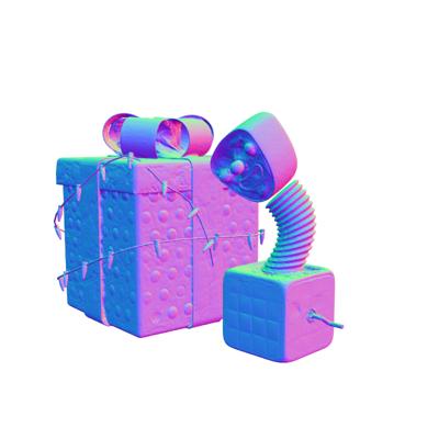
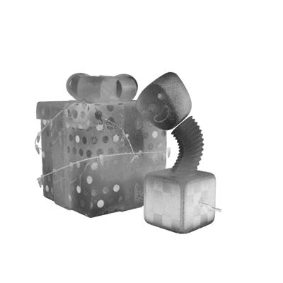
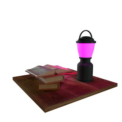
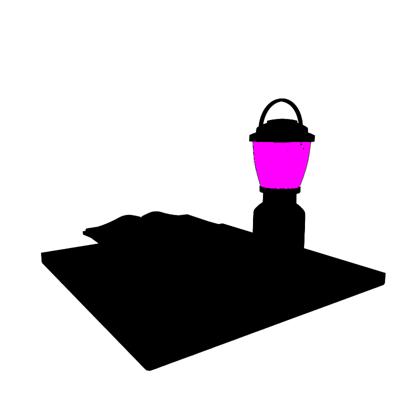
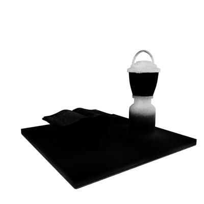
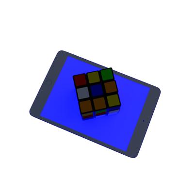
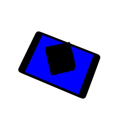
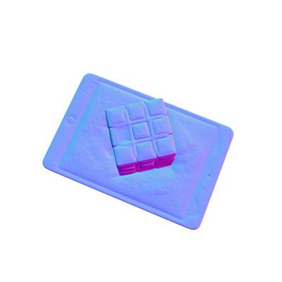
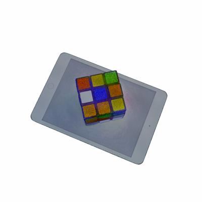
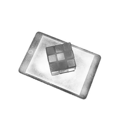
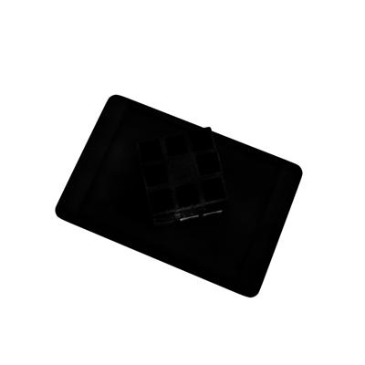
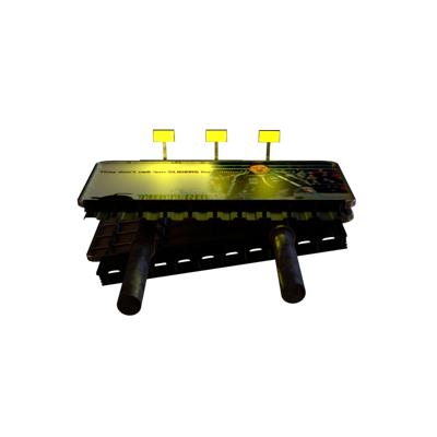
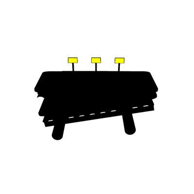
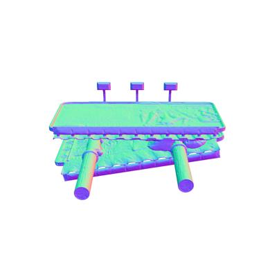
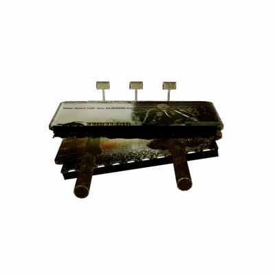
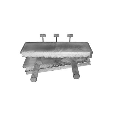
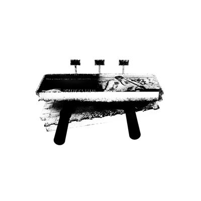
Figure 25: Decomposed scene components on scenes with vivid-colored emissive sources.

	TensoIR	NeILF++	ESR-NeRF	TensoIR	NeILF++	ESR-NeRF
Emission
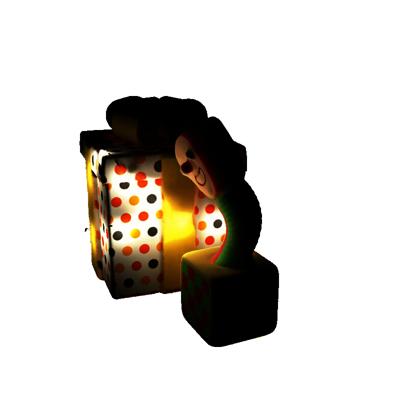
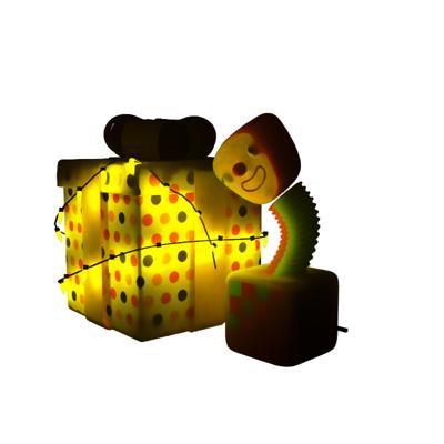
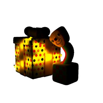
Albedo
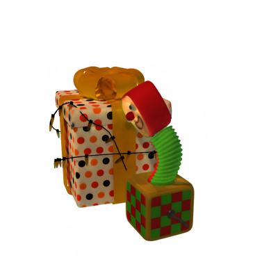
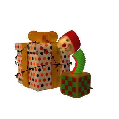
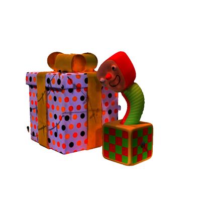
Roughness

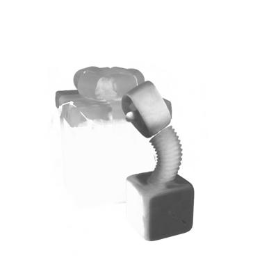
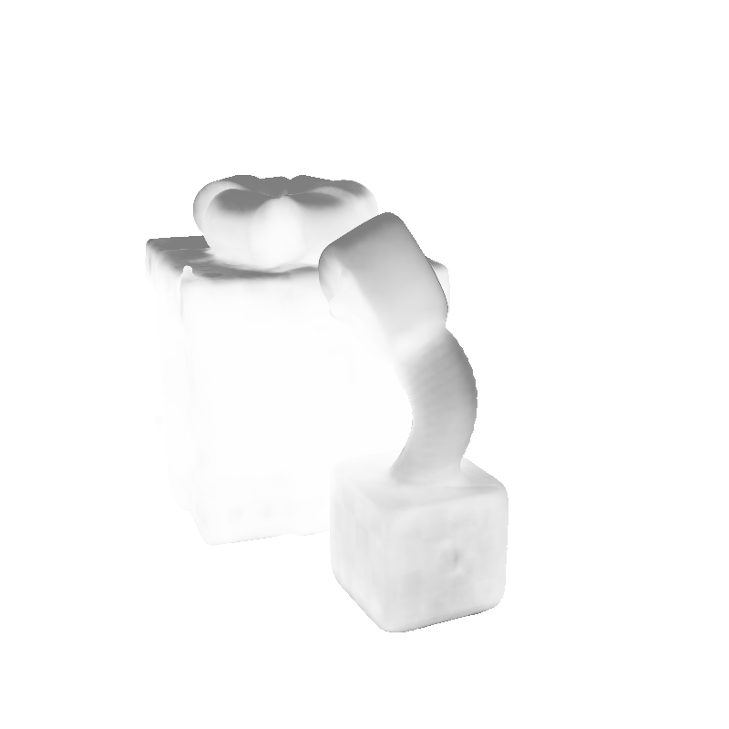
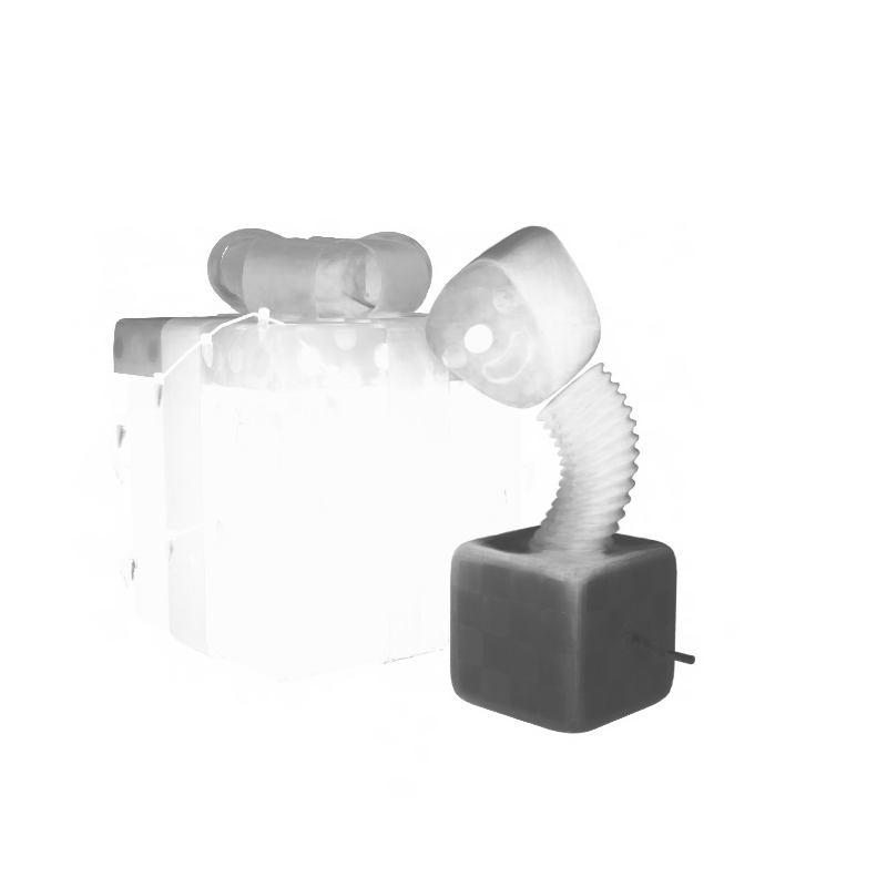
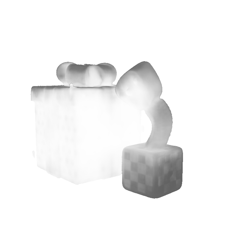
Figure 27: Comparison of identified emissive sources and decomposed BRDF on the Gift scene. Left: Gift white. Right: Gift vivid.

	TensoIR	NeILF++	ESR-NeRF	TensoIR	NeILF++	ESR-NeRF
Emission
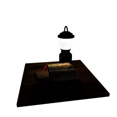
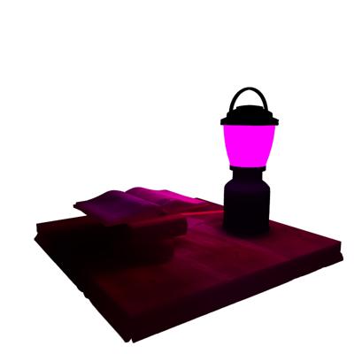
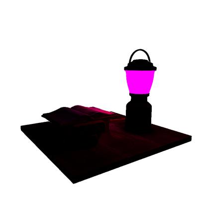
Albedo
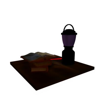
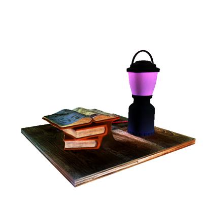
Roughness

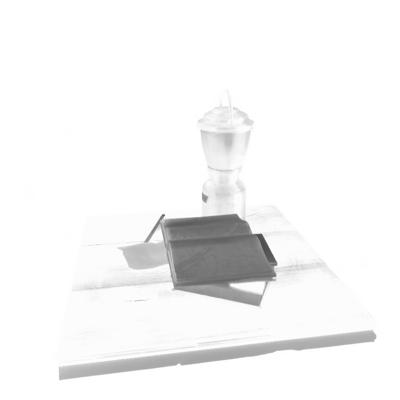
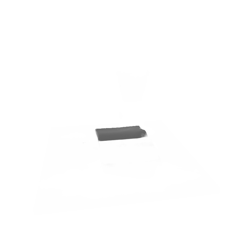
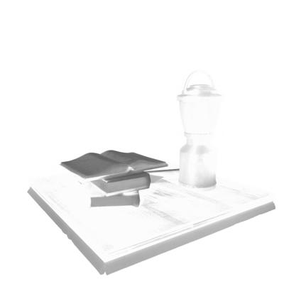
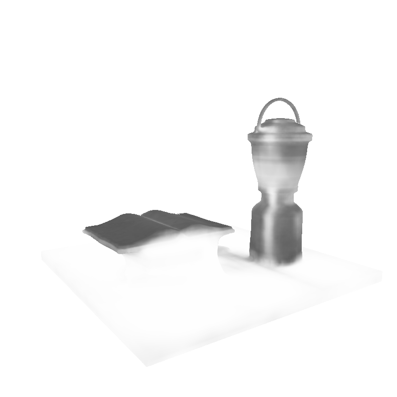
Figure 28: Comparison of identified emissive sources and decomposed BRDF on the Book scene. Left: Book white. Right: Book vivid.

	TensoIR	NeILF++	ESR-NeRF	TensoIR	NeILF++	ESR-NeRF
Emission
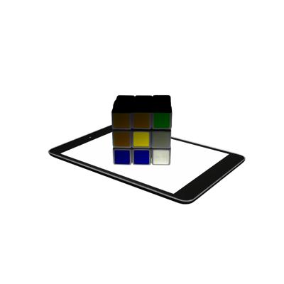
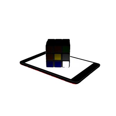
Albedo
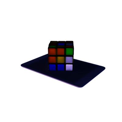
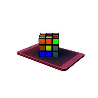
Roughness

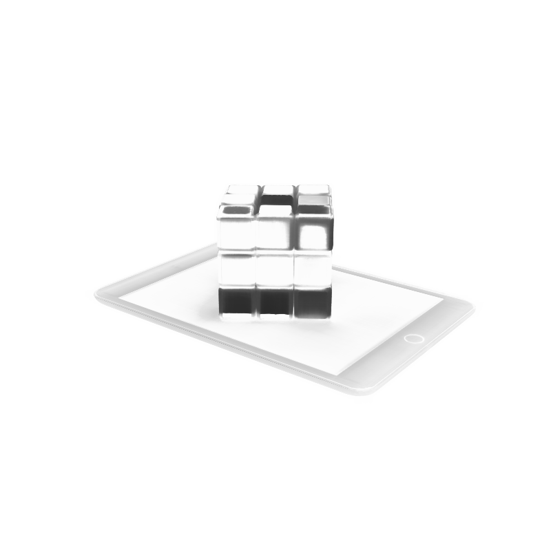
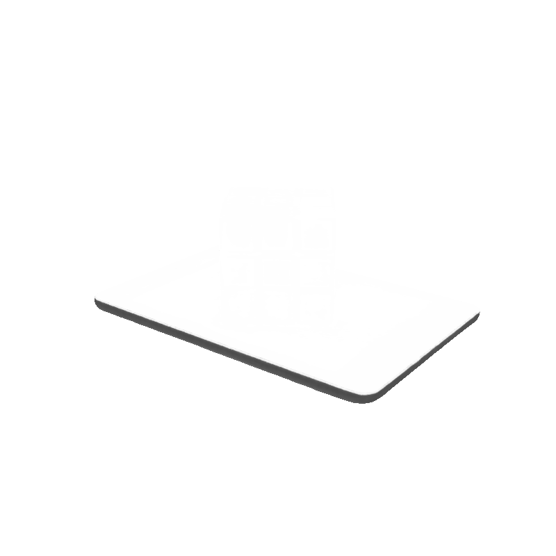
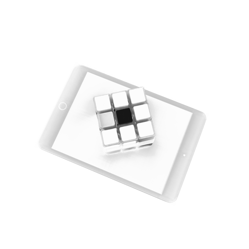
Figure 29: Comparison of identified emissive sources and decomposed BRDF on the Cube scene. Left: Cube white. Right: Cube vivid.

	TensoIR	NeILF++	ESR-NeRF	TensoIR	NeILF++	ESR-NeRF
Emission
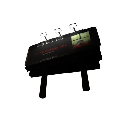
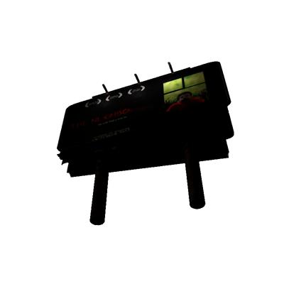
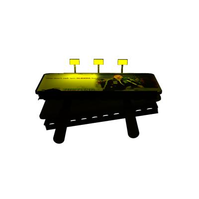
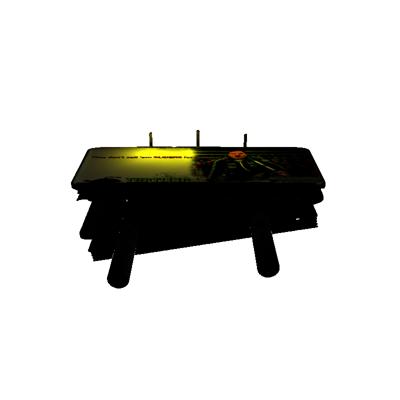
Albedo
Roughness

Figure 30: Comparison of identified emissive sources and decomposed BRDF on the Billboard scene. Left: Billboard white. Right: Billboard vivid.

Image	Normal	Base Color	Roughness	Metallic	Env. Map

Image	Normal	Base Color	Roughness	Metallic	Env. Map

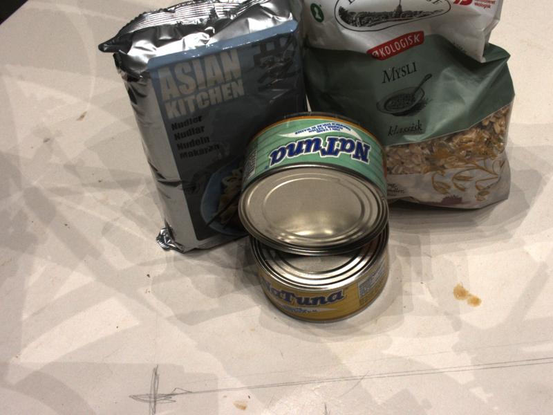
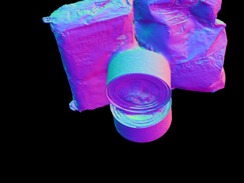
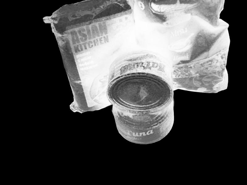
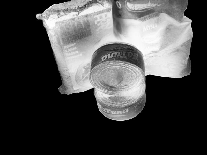
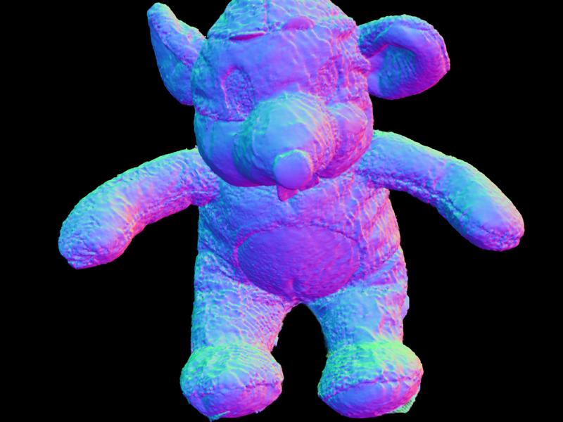
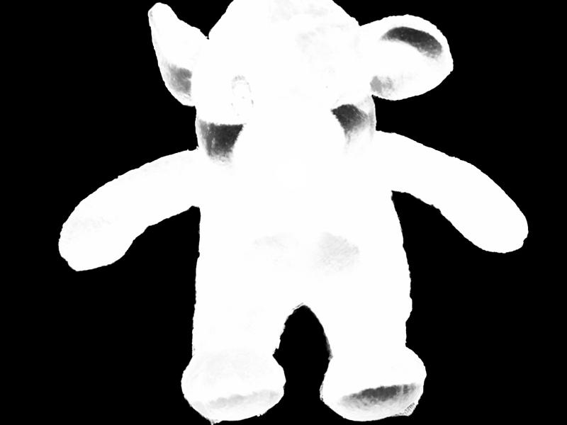
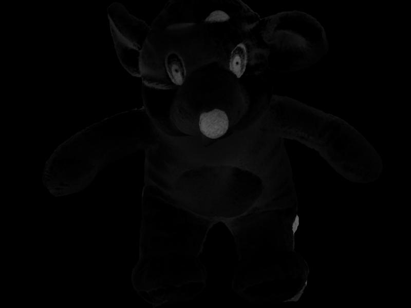
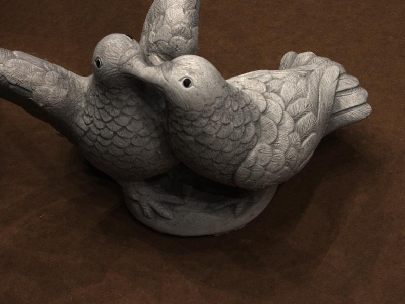
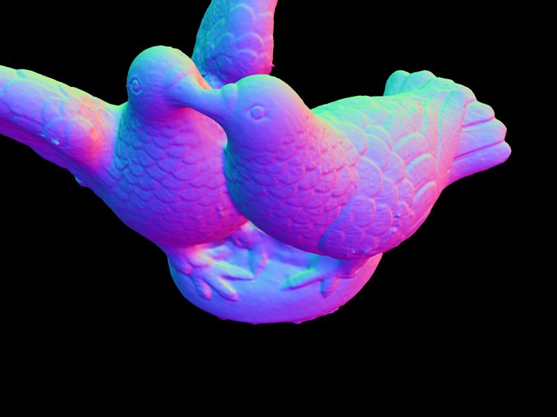
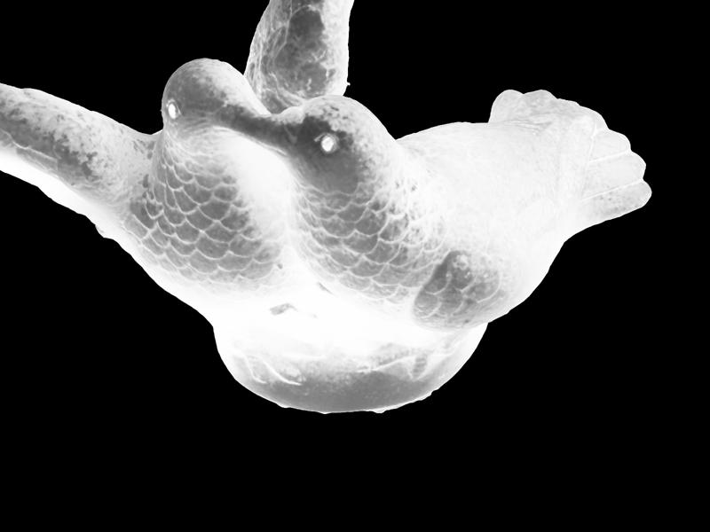
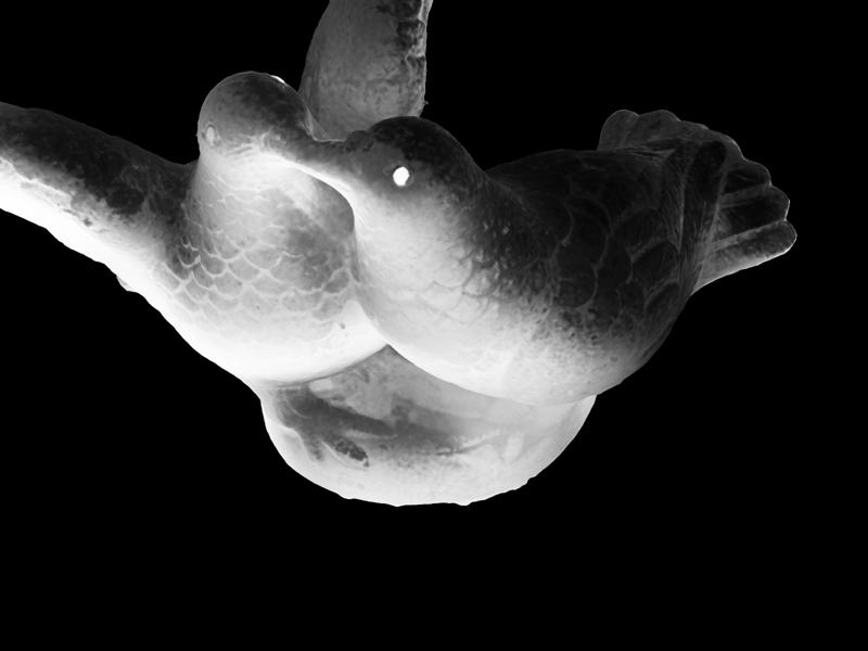
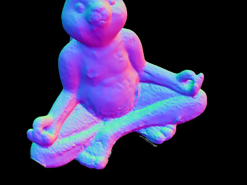
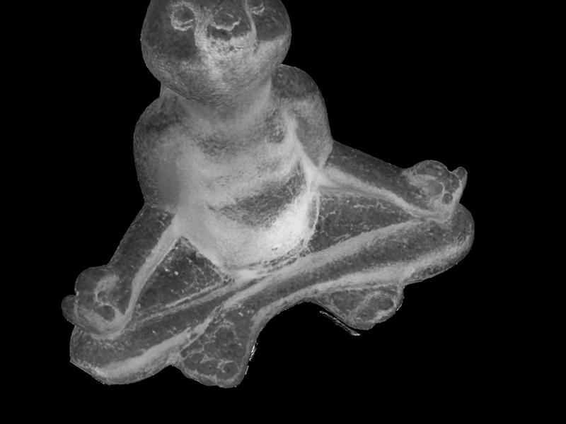
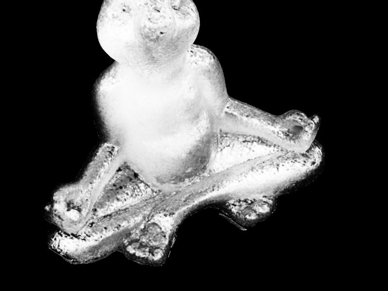
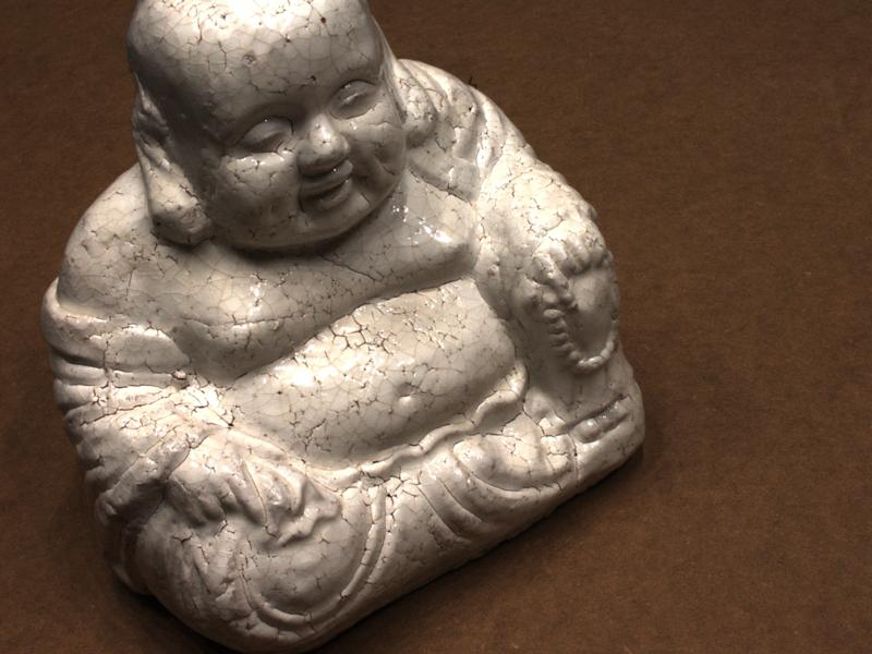
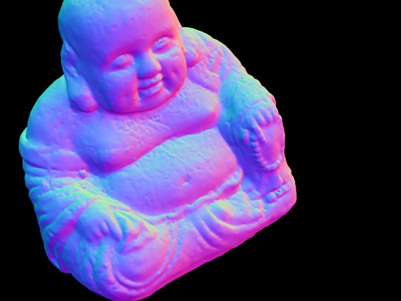
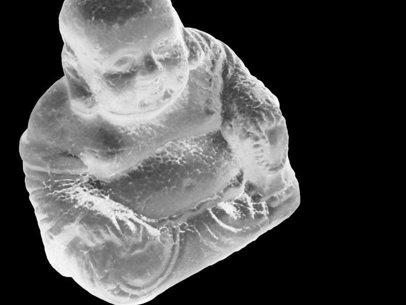
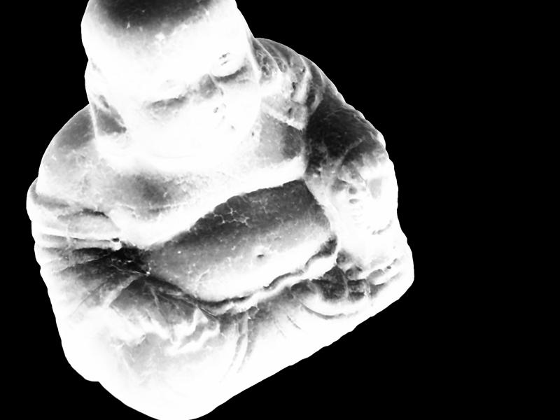
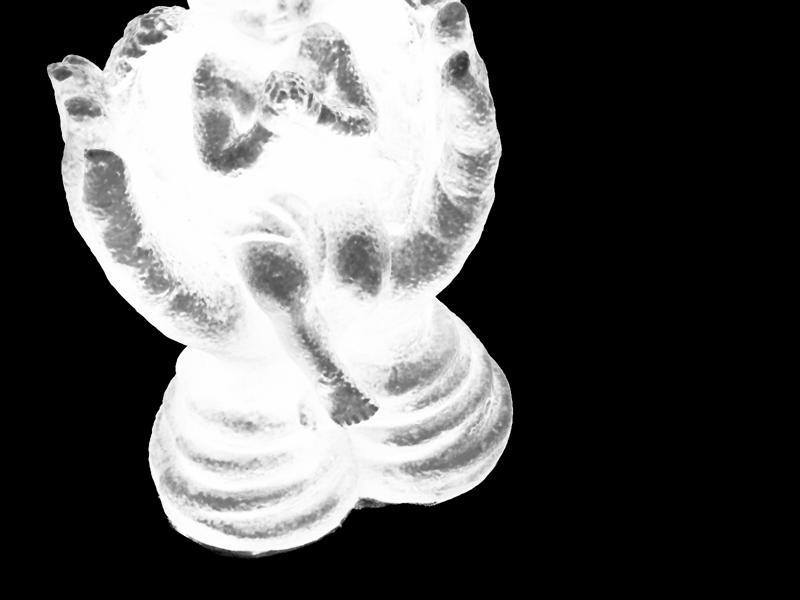
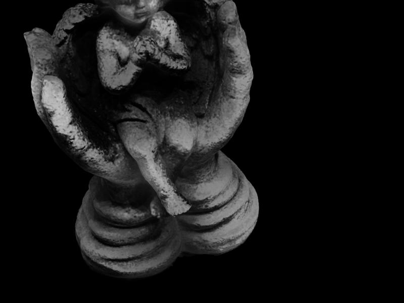
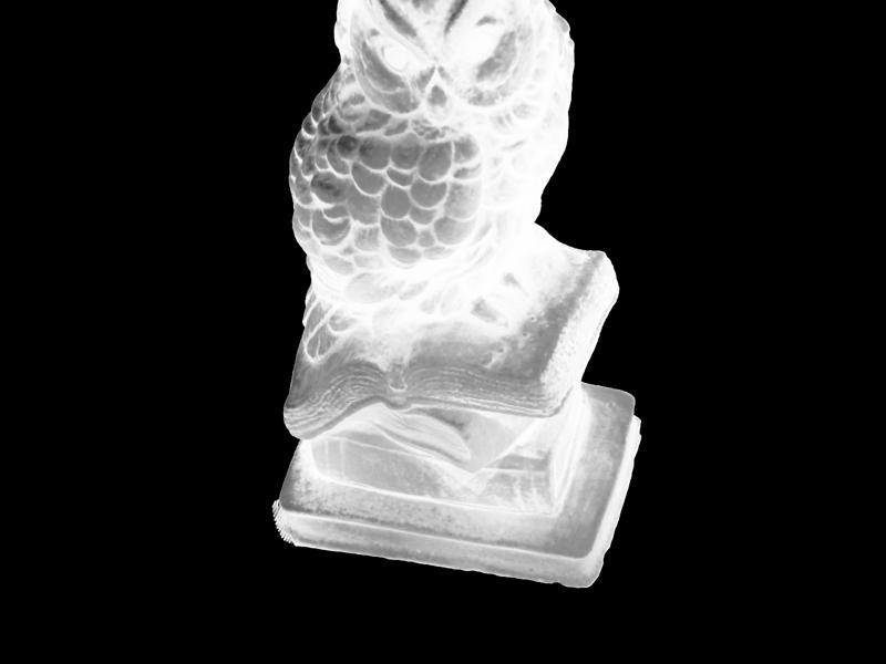
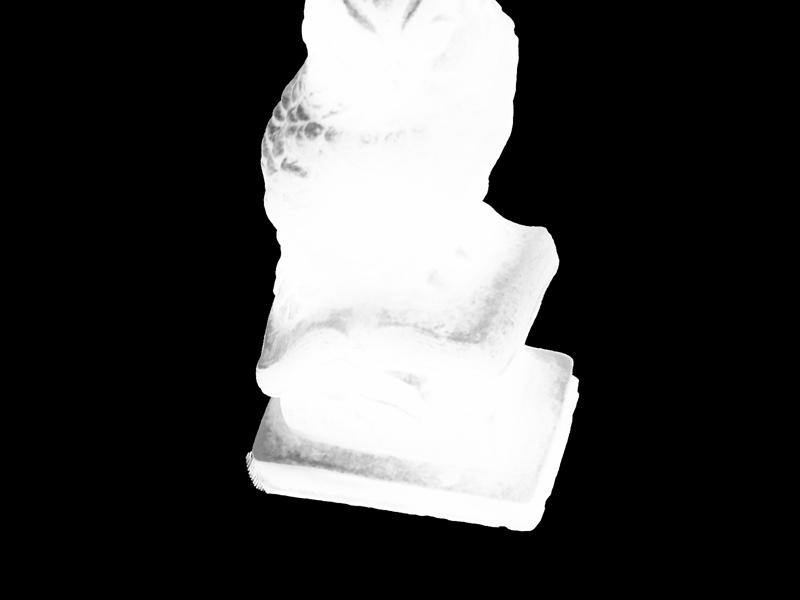
Figure 32: Decomposed scene components on DTU scenes without emissive sources.

Image	Intensity Edit	Color Edit	Intensity & Color Edit	Image	Intensity Edit	Color Edit	Intensity & Color Edit

Image	Intensity Edit	Color Edit	Intensity & Color Edit	Image	Intensity Edit	Color Edit	Intensity & Color Edit

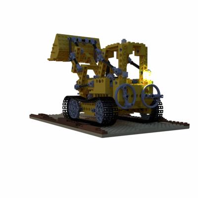
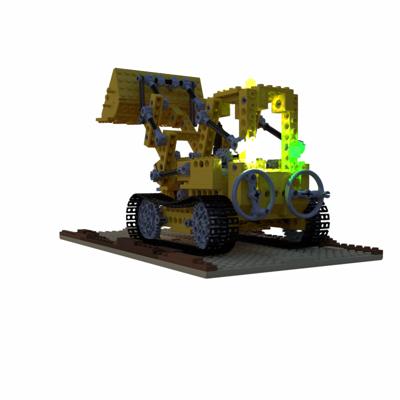
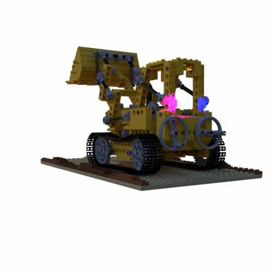
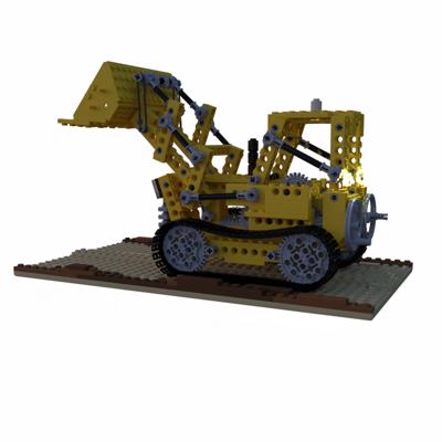
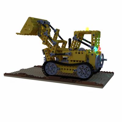
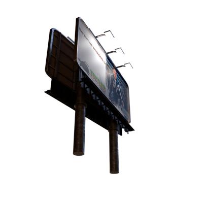
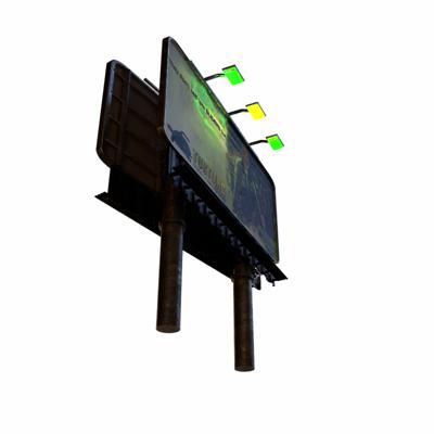
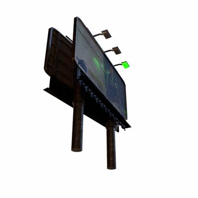
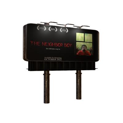
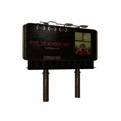
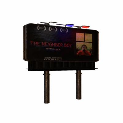
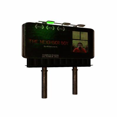
Figure 35: Individual emissive sources control. Left: through fine-tuning radiance fields, Right: computing direct illumination from reconstructed emissive sources.

Image	Intensity Edit	Color Edit	Intensity & Color Edit

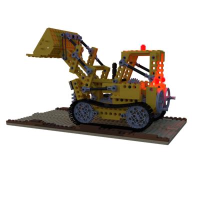
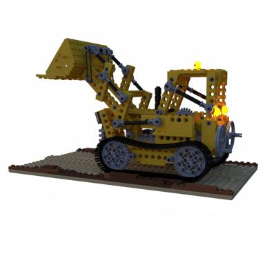
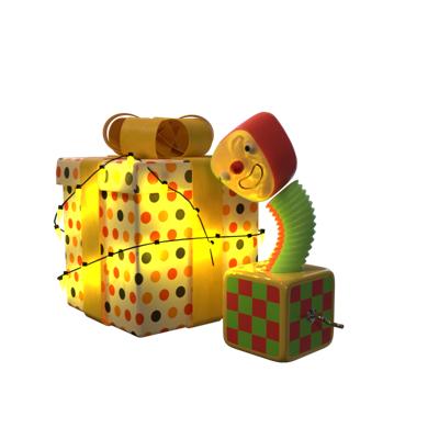
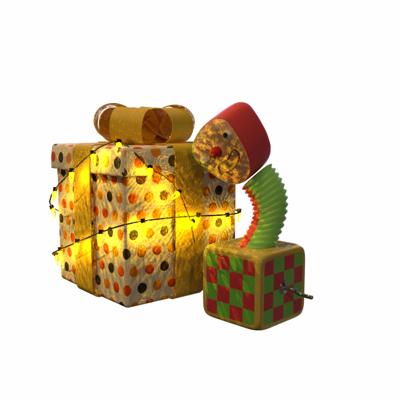
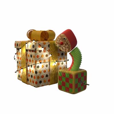
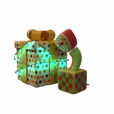
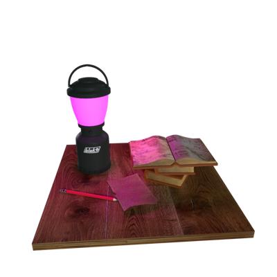
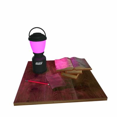
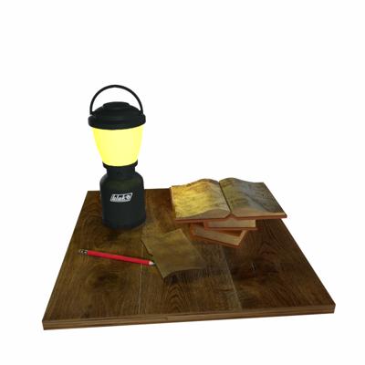
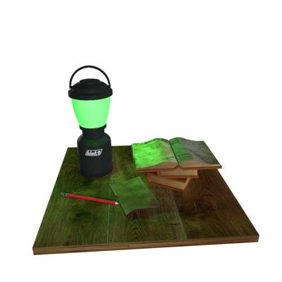
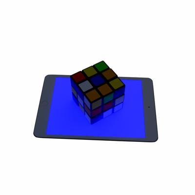
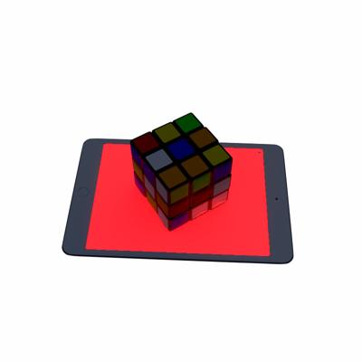
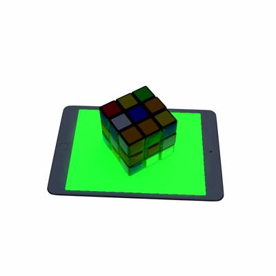
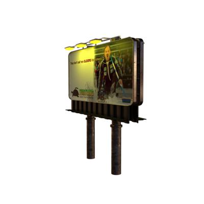
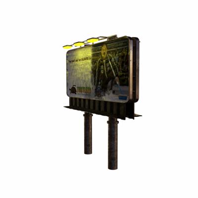
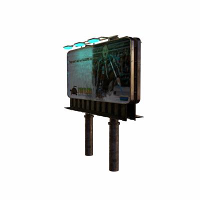
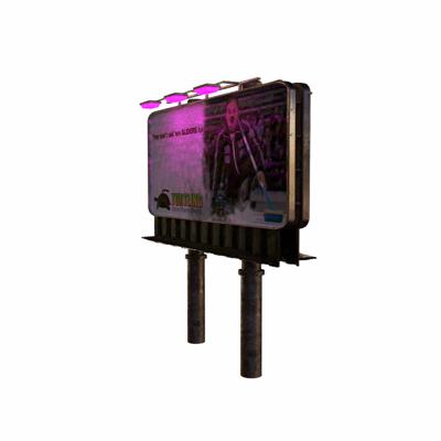
Figure 36: Re-lighting scenes containing vivid-colored emissive sources by computing direct illumination from reconstructed emissive sources.

	White colored
	Lego (C)		Lego (I)		Gift		Book		Cube		Billboard (C)		Billboard (I)		Balls
	PSNR	LPIPS	PSNR	LPIPS	PSNR	LPIPS	PSNR	LPIPS	PSNR	LPIPS	PSNR	LPIPS	PSNR	LPIPS	PSNR	LPIPS
NV	37.77	0.0082	37.77	0.0082	37.72	0.0060	44.95	0.0032	43.60	0.0022	36.23	0.0109	36.23	0.0109	32.49	0.0190
NV + I	32.53	0.0175	29.50	0.0261	27.27	0.0163	30.29	0.0166	31.47	0.0097	29.50	0.0188	30.31	0.0216	29.03	0.0281
NV + C	32.27	0.0220	29.93	0.0259	31.28	0.0140	34.92	0.0123	35.08	0.0083	31.17	0.0197	27.66	0.0322	31.55	0.0221
NV + I + C	29.12	0.0291	30.44	0.0248	31.02	0.0151	34.80	0.0128	34.04	0.0093	31.22	0.0200	31.94	0.0245	30.44	0.0239

Table 9: Editing performance on scenes with white-colored emissive sources by using the fine-tuning method. (C) denotes collective adjustments of emissive sources, while (I) represents individual adjustments of emissive sources. NV denotes novel view synthesis, I denotes intensity editing, and C denotes color editing. A higher PSNR or lower LPIPS value is better.

	White colored
	Lego (C)		Lego (I)		Gift		Book		Cube		Billboard (C)		Billboard (I)		Balls
	PSNR	LPIPS	PSNR	LPIPS	PSNR	LPIPS	PSNR	LPIPS	PSNR	LPIPS	PSNR	LPIPS	PSNR	LPIPS	PSNR	LPIPS
NV	37.77	0.0082	37.77	0.0082	37.72	0.0060	44.95	0.0032	43.60	0.0022	36.23	0.0109	36.23	0.0109	32.49	0.0190
NV + I	27.77	0.0329	29.00	0.0293	22.77	0.0461	28.85	0.0327	24.71	0.0382	26.49	0.0422	31.14	0.0249	28.41	0.0411
NV + C	30.44	0.0292	29.96	0.0284	27.00	0.0316	33.71	0.0191	30.34	0.0229	29.90	0.0328	31.14	0.0320	30.74	0.0282
NV + I + C	30.17	0.0307	30.44	0.0275	27.49	0.0318	33.40	0.0203	27.67	0.0312	29.80	0.0313	32.92	0.0242	29.94	0.0311

Table 10: Editing performance on scenes with white-colored emissive sources by computing direct illumination from reconstructed emissive sources. (C) denotes collective adjustments of emissive sources, while (I) represents individual adjustments of emissive sources. NV denotes novel view synthesis, I denotes intensity editing, and C denotes color editing. A higher PSNR or lower LPIPS value is better.

	Vivid colored
	Lego (C)		Gift		Book		Cube		Billboard (C)		Balls
	PSNR	LPIPS	PSNR	LPIPS	PSNR	LPIPS	PSNR	LPIPS	PSNR	LPIPS	PSNR	LPIPS
NV	39.76	0.0062	38.31	0.0055	44.97	0.0033	45.13	0.0016	34.47	0.0165	32.78	0.0180
NV + I	35.00	0.0154	28.70	0.0163	32.86	0.0141	35.54	0.0072	28.56	0.0288	30.78	0.0231
NV + C	22.80	0.0916	26.00	0.0312	29.11	0.0371	22.50	0.0379	27.82	0.0347	30.05	0.0259
NV + I + C	23.28	0.0873	26.64	0.0290	28.15	0.0419	24.10	0.0361	27.12	0.0367	26.91	0.0329

Table 11: Editing performance on scenes with vivid-colored emissive sources by using the fine-tuning method. (C) denotes collective adjustments of emissive sources. NV denotes novel view synthesis, I denotes intensity editing, and C denotes color editing. A higher PSNR or lower LPIPS value is better.

	Vivid colored
	Lego (C)		Gift		Book		Cube		Billboard (C)		Balls
	PSNR	LPIPS	PSNR	LPIPS	PSNR	LPIPS	PSNR	LPIPS	PSNR	LPIPS	PSNR	LPIPS
NV	39.76	0.0062	38.31	0.0055	44.97	0.0033	45.13	0.0016	34.47	0.0165	32.78	0.0180
NV + I	29.21	0.0330	24.97	0.0378	31.78	0.0216	27.44	0.0314	28.19	0.0356	27.20	0.0352
NV + C	27.41	0.0330	26.49	0.0318	33.95	0.0198	28.81	0.0260	28.51	0.0326	29.57	0.0301
NV + I + C	27.27	0.0348	26.80	0.0312	33.28	0.0232	24.62	0.0447	28.56	0.0329	24.89	0.0388

Table 12: Editing performance on scenes with vivid-colored emissive sources by computing direct illumination from reconstructed emissive sources. (C) denotes collective adjustments of emissive sources. NV denotes novel view synthesis, I denotes intensity editing, and C denotes color editing. A higher PSNR or lower LPIPS value is better.

Image	Edit	G.T

Image	Normal	Rendered

References

- Attal et al. [2022] Benjamin Attal, Jia-Bin Huang, Michael Zollhöfer, Johannes Kopf, and Changil Kim. Learning neural light fields with ray-space embedding. In CVPR, 2022.
- Azinovic et al. [2019] Dejan Azinovic, Tzu-Mao Li, Anton Kaplanyan, and Matthias Nießner. Inverse path tracing for joint material and lighting estimation. In CVPR, 2019.
- Barron et al. [2021] Jonathan T Barron, Ben Mildenhall, Matthew Tancik, Peter Hedman, Ricardo Martin-Brualla, and Pratul P Srinivasan. Mip-nerf: A multiscale representation for anti-aliasing neural radiance fields. In ICCV, 2021.
- Barron et al. [2022] Jonathan T Barron, Ben Mildenhall, Dor Verbin, Pratul P Srinivasan, and Peter Hedman. Mip-nerf 360: Unbounded anti-aliased neural radiance fields. In CVPR, 2022.
- Barron et al. [2023] Jonathan T. Barron, Ben Mildenhall, Dor Verbin, Pratul P. Srinivasan, and Peter Hedman. Zip-nerf: Anti-aliased grid-based neural radiance fields. In ICCV, 2023.
- Bi et al. [2020] Sai Bi, Zexiang Xu, Pratul Srinivasan, Ben Mildenhall, Kalyan Sunkavalli, Miloš Hašan, Yannick Hold-Geoffroy, David Kriegman, and Ravi Ramamoorthi. Neural reflectance fields for appearance acquisition. In arXiv, 2020.
- Boss et al. [2020] Mark Boss, Varun Jampani, Kihwan Kim, Hendrik Lensch, and Jan Kautz. Two-shot spatially-varying brdf and shape estimation. In CVPR, 2020.
- Boss et al. [2021a] Mark Boss, Raphael Braun, Varun Jampani, Jonathan T. Barron, Ce Liu, and Hendrik P.A. Lensch. Nerd: Neural reflectance decomposition from image collections. In ICCV, 2021a.
- Boss et al. [2021b] Mark Boss, Varun Jampani, Raphael Braun, Ce Liu, Jonathan T. Barron, and Hendrik P.A. Lensch. Neural-pil: Neural pre-integrated lighting for reflectance decomposition. In NeurIPS, 2021b.
- Burley and Studios [2012] Brent Burley and Walt Disney Animation Studios. Physically-based shading at disney. In SIGGRAPH, 2012.
- Cai et al. [2023] Bowen Cai, Jinchi Huang, Rongfei Jia, Chengfei Lv, and Huan Fu. Neuda: Neural deformable anchor for high-fidelity implicit surface reconstruction. In CVPR, 2023.
- Chen et al. [2022] Anpei Chen, Zexiang Xu, Andreas Geiger, Jingyi Yu, and Hao Su. Tensorf: Tensorial radiance fields. In ECCV, 2022.
- Community [2018] Blender Online Community. Blender - a 3D modelling and rendering package. Blender Foundation, Stichting Blender Foundation, Amsterdam, 2018.
- Fridovich-Keil et al. [2022] Sara Fridovich-Keil, Alex Yu, Matthew Tancik, Qinhong Chen, Benjamin Recht, and Angjoo Kanazawa. Plenoxels: Radiance fields without neural networks. In CVPR, 2022.
- Garon et al. [2019] Mathieu Garon, Kalyan Sunkavalli, Sunil Hadap, Nathan Carr, and Jean-Francois Lalonde. Fast spatially-varying indoor lighting estimation. In CVPR, 2019.
- Ge et al. [2023] Wenhang Ge, Tao Hu, Haoyu Zhao, Shu Liu, and Ying-Cong Chen. Ref-neus: Ambiguity-reduced neural implicit surface learning for multi-view reconstruction with reflection. In ICCV, 2023.
- Hadadan et al. [2021] Saeed Hadadan, Shuhong Chen, and Matthias Zwicker. Neural radiosity. In ACM TOG, 2021.
- Hadadan et al. [2023] Saeed Hadadan, Geng Lin, Jan Novák, Fabrice Rousselle, and Matthias Zwicker. Inverse global illumination using a neural radiometric prior. In SIGGRAPH Conference Proceedings, 2023.
- Haefner et al. [2021] Bjoern Haefner, Simon Green, Alan Oursland, Daniel Andersen, Michael Goesele, Daniel Cremers, Richard Newcombe, and Thomas Whelan. Recovering real-world reflectance properties and shading from hdr imagery. In 3DV, 2021.
- Hasselgren et al. [2022] Jon Hasselgren, Nikolai Hofmann, and Jacob Munkberg. Shape, light, and material decomposition from images using monte carlo rendering and denoising. In NeurIPS, 2022.
- IEC [1999] IEC. IEC 61966-2-1:1999. Technical report, International Electrotechnical Commission, 1999.
- Jakob et al. [2022] Wenzel Jakob, Sébastien Speierer, Nicolas Roussel, Merlin Nimier-David, Delio Vicini, Tizian Zeltner, Baptiste Nicolet, Miguel Crespo, Vincent Leroy, and Ziyi Zhang. Mitsuba 3 renderer, 2022. https://mitsuba-renderer.org.
- Jensen et al. [2014] Rasmus Jensen, Anders Dahl, George Vogiatzis, Engil Tola, and Henrik Aanæs. Large scale multi-view stereopsis evaluation. In CVPR, 2014.
- Ji et al. [2022] Chaonan Ji, Tao Yu, Kaiwen Guo, Jingxin Liu, and Yebin Liu. Geometry-aware single-image full-body human relighting. In ECCV, 2022.
- Jin et al. [2023] Haian Jin, Isabella Liu, Peijia Xu, Xiaoshuai Zhang, Songfang Han, Sai Bi, Xiaowei Zhou, Zexiang Xu, and Hao Su. Tensoir: Tensorial inverse rendering. In CVPR, 2023.
- Kajiya [1986] James T. Kajiya. The rendering equation. In SIGGRAPH, 1986.
- Kellnhofer et al. [2021] Petr Kellnhofer, Lars C Jebe, Andrew Jones, Ryan Spicer, Kari Pulli, and Gordon Wetzstein. Neural lumigraph rendering. In CVPR, 2021.
- Kuang et al. [2023] Zhengfei Kuang, Fujun Luan, Sai Bi, Zhixin Shu, Gordon Wetzstein, and Kalyan Sunkavalli. Palettenerf: Palette-based appearance editing of neural radiance fields. In CVPR, 2023.
- Li et al. [2020] Zhengqin Li, Mohammad Shafiei, Ravi Ramamoorthi, Kalyan Sunkavalli, and Manmohan Chandraker. Inverse rendering for complex indoor scenes: Shape, spatially-varying lighting and svbrdf from a single image. In CVPR, 2020.
- Li et al. [2022] Zhengqin Li, Jia Shi, Sai Bi, Rui Zhu, Kalyan Sunkavalli, Miloš Hašan, Zexiang Xu, Ravi Ramamoorthi, and Manmohan Chandraker. Physically-based editing of indoor scene lighting from a single image. In ECCV, 2022.
- Li et al. [2023a] Zhaoshuo Li, Thomas Müller, Alex Evans, Russell H Taylor, Mathias Unberath, Ming-Yu Liu, and Chen-Hsuan Lin. Neuralangelo: High-fidelity neural surface reconstruction. In CVPR, 2023a.
- Li et al. [2023b] Zhen Li, Lingli Wang, Mofang Cheng, Cihui Pan, and Jiaqi. Yang. Multi-view inverse rendering for large-scale real-world indoor scenes. In CVPR, 2023b.
- Liang et al. [2023] Ruofan Liang, Huiting Chen, Chunlin Li, Fan Chen, Selvakumar Panneer, and Nandita Vijaykumar. Envidr: Implicit differentiable renderer with neural environment lighting. In ICCV, 2023.
- Luan et al. [2021] Fujun Luan, Shuang Zhao, Kavita Bala, and Zhao Dong. Unified shape and svbrdf recovery using differentiable monte carlo rendering. In EGSR, 2021.
- Lyu et al. [2022] Linjie Lyu, Ayush Tewari, Thomas Leimkuehler, Marc Habermann, and Christian Theobalt. Neural radiance transfer fields for relightable novel-view synthesis with global illumination. In ECCV, 2022.
- Lyu et al. [2023] Linjie Lyu, Ayush Tewari, Marc Habermann, Shunsuke Saito, Michael Zollhöfer, Thomas Leimküehler, and Christian Theobalt. Diffusion posterior illumination for ambiguity-aware inverse rendering. In ACM TOG, 2023.
- Mai et al. [2023] Alexander Mai, Dor Verbin, Falko Kuester, and Sara Fridovich-Keil. Neural microfacet fields for inverse rendering. In ICCV, 2023.
- Martin-Brualla et al. [2021] Ricardo Martin-Brualla, Noha Radwan, Mehdi S. M. Sajjadi, Jonathan T. Barron, Alexey Dosovitskiy, and Daniel Duckworth. Nerf in the wild: Neural radiance fields for unconstrained photo collections. In CVPR, 2021.
- Max [1995] Nelson Max. Optical models for direct volume rendering. IEEE Transactions on Visualization and Computer Graphics, 1(2):99–108, 1995.
- Mildenhall et al. [2020] Ben Mildenhall, Pratul P. Srinivasan, Matthew Tancik, Jonathan T. Barron, Ravi Ramamoorthi, and Ren Ng. Nerf: Representing scenes as neural radiance fields for view synthesis. In ECCV, 2020.
- Müller et al. [2022] Thomas Müller, Alex Evans, Christoph Schied, and Alexander Keller. Instant neural graphics primitives with a multiresolution hash encoding. In ACM TOG, 2022.
- Munkberg et al. [2022] Jacob Munkberg, Jon Hasselgren, Tianchang Shen, Jun Gao, Wenzheng Chen, Alex Evans, Thomas Müller, and Sanja Fidler. Extracting triangular 3d models, materials, and lighting from images. In CVPR, 2022.
- Niemeyer et al. [2020] Michael Niemeyer, Lars Mescheder, Michael Oechsle, and Andreas Geiger. Differentiable volumetric rendering: Learning implicit 3d representations without 3d supervision. In CVPR, 2020.
- Oechsle et al. [2021] Michael Oechsle, Songyou Peng, and Andreas Geiger. Unisurf: Unifying neural implicit surfaces and radiance fields for multi-view reconstruction. In ICCV, 2021.
- Ost et al. [2022] Julian Ost, Issam Laradji, Alejandro Newell, Yuval Bahat, and Felix Heide. Neural point light fields. In CVPR, 2022.
- Pandey et al. [2021] Rohit Pandey, Sergio Orts-Escolano, Chloe LeGendre, Christian Haene, Sofien Bouaziz, Christoph Rhemann, Paul Debevec, and Seann Fanello. Total relighting: Learning to relight portraits for background replacement. In ACM TOG, 2021.
- Park et al. [2019] Jeong Joon Park, Peter Florence, Julian Straub, Richard Newcombe, and Steven Lovegrove. Deepsdf: Learning continuous signed distance functions for shape representation. In CVPR, 2019.
- Philip et al. [2021] Julien Philip, Sébastien Morgenthaler, Michaël Gharbi, and George Drettakis. Free-viewpoint indoor neural relighting from multi-view stereo. In ACM TOG, 2021.
- Piala and Clark [2021] Martin Piala and Ronald Clark. Terminerf: Ray termination prediction for efficient neural rendering. In 3DV, 2021.
- Rudnev et al. [2022] Viktor Rudnev, Mohamed Elgharib, William Smith, Lingjie Liu, Vladislav Golyanik, and Christian Theobalt. Nerf for outdoor scene relighting. In ECCV, 2022.
- Schonberger and Frahm [2016] Johannes L. Schonberger and Jan-Michael Frahm. Structure-from-motion revisited. In CVPR, 2016.
- Sitzmann et al. [2020] Vincent Sitzmann, Julien N.P. Martel, Alexander W. Bergman, David B. Lindell, and Gordon Wetzstein. Implicit neural representations with periodic activation functions. In NeurIPS, 2020.
- Sitzmann et al. [2021] Vincent Sitzmann, Semon Rezchikov, Bill Freeman, Josh Tenenbaum, and Fredo Durand. Light field networks: Neural scene representations with single-evaluation rendering. In NeurIPS, 2021.
- Smith [1978] Alvy Ray Smith. Color gamut transform pairs. In ACM TOG, 1978.
- Srinivasan et al. [2021] Pratul P. Srinivasan, Boyang Deng, Xiuming Zhang, Matthew Tancik, Ben Mildenhall, and Jonathan T. Barron. Nerv: Neural reflectance and visibility fields for relighting and view synthesis. In CVPR, 2021.
- Srinivasan et al. [2023] Pratul P. Srinivasan, Stephan J. Garbin, Dor Verbin, Jonathan T. Barron, and Ben Mildenhall. Nuvo: Neural uv mapping for unruly 3d representations. arXiv, 2023.
- Suhail et al. [2022] Mohammed Suhail, Carlos Esteves, Leonid Sigal, and Ameesh Makadia. Light field neural rendering. In CVPR, 2022.
- Sun et al. [2022a] Cheng Sun, Min Sun, and Hwann-Tzong Chen. Direct voxel grid optimization: Super-fast convergence for radiance fields reconstruction. In CVPR, 2022a.
- Sun et al. [2023] Cheng Sun, Guangyan Cai, Zhengqin Li, Kai Yan, Cheng Zhang, Carl Marshall, Jia-Bin Huang, Shuang Zhao, and Zhao Dong. Neural-pbir reconstruction of shape, material, and illumination. In ICCV, 2023.
- Sun et al. [2022b] Jiaming Sun, Xi Chen, Qianqian Wang, Zhengqi Li, Hadar Averbuch-Elor, Xiaowei Zhou, and Noah Snavely. Neural 3D reconstruction in the wild. In SIGGRAPH Conference Proceedings, 2022b.
- Sun et al. [2021] Tiancheng Sun, Kai-En Lin, Sai Bi, Zexiang Xu, and Ravi Ramamoorthi. Nelf: Neural light-transport field for portrait view synthesis and relighting. In EGSR, 2021.
- Tancik et al. [2020] Matthew Tancik, Pratul P. Srinivasan, Ben Mildenhall, Sara Fridovich-Keil, Nithin Raghavan, Utkarsh Singhal, Ravi Ramamoorthi, Jonathan T. Barron, and Ren Ng. Fourier features let networks learn high frequency functions in low dimensional domains. In NeurIPS, 2020.
- Tang et al. [2023] Jiaxiang Tang, Hang Zhou, Xiaokang Chen, Tianshu Hu, Errui Ding, Jingdong Wang, and Gang Zeng. Delicate textured mesh recovery from nerf via adaptive surface refinement. In ICCV, 2023.
- Tewari et al. [2020] Ayush Tewari, Ohad Fried, Justus Thies, Vincent Sitzmann, Stephen Lombardi, Kalyan Sunkavalli, Ricardo Martin-Brualla, Tomas Simon, Jason Saragih, Matthias Nießner, et al. State of the art on neural rendering. In CGF, 2020.
- Tewari et al. [2022] Ayush Tewari, Justus Thies, Ben Mildenhall, Pratul Srinivasan, Edgar Tretschk, Wang Yifan, Christoph Lassner, Vincent Sitzmann, Ricardo Martin-Brualla, Stephen Lombardi, et al. Advances in neural rendering. In CGF, 2022.
- Toschi et al. [2023] Marco Toschi, Riccardo De Matteo, Riccardo Spezialetti, Daniele De Gregorio, Luigi Di Stefano, and Samuele Salti. Relight my nerf: A dataset for novel view synthesis and relighting of real world objects. In CVPR, 2023.
- Verbin et al. [2022] Dor Verbin, Peter Hedman, Ben Mildenhall, Todd Zickler, Jonathan T Barron, and Pratul P Srinivasan. Ref-nerf: Structured view-dependent appearance for neural radiance fields. In CVPR, 2022.
- Walter et al. [2007] Bruce Walter, Stephen R. Marschner, Hongsong Li, and Kenneth E. Torrance. Microfacet models for refraction through rough surfaces. In Proceedings of the 18th Eurographics Conference on Rendering Techniques, 2007.
- Wang et al. [2023a] Dongqing Wang, Tong Zhang, and Sabine Süsstrunk. Nemto: Neural environment matting for novel view and relighting synthesis of transparent objects. In ICCV, 2023a.
- Wang et al. [2009] Jiaping Wang, Peiran Ren, Minmin Gong, John Snyder, and Baining Guo. All-frequency rendering of dynamic, spatially-varying reflectance. ACM TOG, 2009.
- Wang et al. [2021a] Peng Wang, Lingjie Liu, Yuan Liu, Christian Theobalt, Taku Komura, and Wenping Wang. Neus: Learning neural implicit surfaces by volume rendering for multi-view reconstruction. In NeurIPS, 2021a.
- Wang et al. [2022a] Shaofei Wang, Katja Schwarz, Andreas Geiger, and Siyu Tang. Arah: Animatable volume rendering of articulated human sdfs. In ECCV, 2022a.
- Wang et al. [2023b] Yiming Wang, Qin Han, Marc Habermann, Kostas Daniilidis, Christian Theobalt, and Lingjie Liu. Neus2: Fast learning of neural implicit surfaces for multi-view reconstruction. In ICCV, 2023b.
- Wang et al. [2021b] Zian Wang, Jonah Philion, Sanja Fidler, and Jan Kautz. Learning indoor inverse rendering with 3d spatially-varying lighting. In ICCV, 2021b.
- Wang et al. [2022b] Zian Wang, Wenzheng Chen, David Acuna, Jan Kautz, and Sanja Fidler. Neural light field estimation for street scenes with differentiable virtual object insertion. In ECCV, 2022b.
- Wang et al. [2023c] Zian Wang, Tianchang Shen, Jun Gao, Shengyu Huang, Jacob Munkberg, Jon Hasselgren, Zan Gojcic, Wenzheng Chen, and Sanja Fidler. Neural fields meet explicit geometric representations for inverse rendering of urban scenes. In CVPR, 2023c.
- Weber et al. [2022] Henrique Weber, Mathieu Garon, and Jean-François Lalonde. Editable indoor lighting estimation. In ECCV, 2022.
- Wu et al. [2023a] Haoqian Wu, Zhipeng Hu, Lincheng Li, Yongqiang Zhang, Changjie Fan, and Xin Yu. Nefii: Inverse rendering for reflectance decomposition with near-field indirect illumination. In CVPR, 2023a.
- Wu et al. [2023b] Liwen Wu, Rui Zhu, Mustafa B. Yaldiz, Yinhao Zhu, Hong Cai, Janarbek Matai, Fatih Porikli, Tzu-Mao Li, Manmohan Chandraker, and Ravi Ramamoorthi. Factorized inverse path tracing for efficient and accurate material-lighting estimation. In ICCV, 2023b.
- Wu et al. [2022] Qianyi Wu, Xian Liu, Yuedong Chen, Kejie Li, Chuanxia Zheng, Jianfei Cai, and Jianmin Zheng. Object-compositional neural implicit surfaces. In ECCV, 2022.
- Wu et al. [2023c] Qianyi Wu, Kaisiyuan Wang, Kejie Li, Jianmin Zheng, and Jianfei Cai. Objectsdf++: Improved object-compositional neural implicit surfaces. In ICCV, 2023c.
- Wu et al. [2023d] Tong Wu, Jia-Mu Sun, Yu-Kun Lai, and Lin Gao. De-nerf: Decoupled neural radiance fields for view-consistent appearance editing and high-frequency environmental relighting. In SIGGRAPH ASIA Conference Proceedings, 2023d.
- Wu et al. [2023e] Tong Wu, Jiaqi Wang, Xingang Pan, Xudong Xu, Christian Theobalt, Ziwei Liu, and Dahua Lin. Voxurf: Voxel-based efficient and accurate neural surface reconstruction. In ICLR, 2023e.
- Xiangli et al. [2022] Yuanbo Xiangli, Linning Xu, Xingang Pan, Nanxuan Zhao, Anyi Rao, Christian Theobalt, Bo Dai, and Dahua Lin. Bungeenerf: Progressive neural radiance field for extreme multi-scale scene rendering. In ECCV, 2022.
- Xu et al. [2023] Yingyan Xu, Gaspard Zoss, Prashanth Chandran, Markus Gross, Derek Bradley, and Paulo Gotardo. Renerf: Relightable neural radiance fields with nearfield lighting. In ICCV, 2023.
- Yang et al. [2022a] Wenqi Yang, Guanying Chen, Chaofeng Chen, Zhenfang Chen, and Kwan-Yee K. Wong. Ps-nerf: Neural inverse rendering for multi-view photometric stereo. In ECCV, 2022a.
- Yang et al. [2022b] Wenqi Yang, Guanying Chen, Chaofeng Chen, Zhenfang Chen, and Kwan-Yee K. Wong. S3-nerf: Neural reflectance field from shading and shadow under a single viewpoint. In NeurIPS, 2022b.
- Yao et al. [2022] Yao Yao, Jingyang Zhang, Jingbo Liu, Yihang Qu, Tian Fang, David McKinnon, Yanghai Tsin, and Long Quan. Neilf: Neural incident light field for material and lighting estimation. In ECCV, 2022.
- Yariv et al. [2020] Lior Yariv, Yoni Kasten, Dror Moran, Meirav Galun, Matan Atzmon, Basri Ronen, and Yaron Lipman. Multiview neural surface reconstruction by disentangling geometry and appearance. In NeurIPS, 2020.
- Yariv et al. [2021] Lior Yariv, Jiatao Gu, Yoni Kasten, and Yaron Lipman. Volume rendering of neural implicit surfaces. In NeurIPS, 2021.
- Yu et al. [2021] Alex Yu, Ruilong Li, Matthew Tancik, Hao Li, Ren Ng, and Angjoo Kanazawa. PlenOctrees for real-time rendering of neural radiance fields. In ICCV, 2021.
- Zeng et al. [2023] Chong Zeng, Guojun Chen, Yue Dong, Pieter Peers, Hongzhi Wu, and Xin Tong. Relighting neural radiance fields with shadow and highlight hints. In SIGGRAPH Conference Proceedings, 2023.
- Zhang et al. [2023a] Jingyang Zhang, Yao Yao, Shiwei Li, Jingbo Liu, Tian Fang, David McKinnon, Yanghai Tsin, and Long Quan. Neilf++: Inter-reflectable light fields for geometry and material estimation. In ICCV, 2023a.
- Zhang et al. [2020] Kai Zhang, Gernot Riegler, Noah Snavely, and Vladlen Koltun. Nerf++: Analyzing and improving neural radiance fields. arXiv preprint arXiv:2010.07492, 2020.
- Zhang et al. [2021a] Kai Zhang, Fujun Luan, Qianqian Wang, Kavita Bala, and Noah Snavely. Physg: Inverse rendering with spherical gaussians for physics-based material editing and relighting. In CVPR, 2021a.
- Zhang et al. [2022a] Kai Zhang, Fujun Luan, Zhengqi Li, and Noah Snavely. Iron: Inverse rendering by optimizing neural sdfs and materials from photometric images. In CVPR, 2022a.
- Zhang et al. [2021b] Xiuming Zhang, Sean Fanello, Yun-Ta Tsai, Tiancheng Sun, Tianfan Xue, Rohit Pandey, Sergio Orts-Escolano, Philip Davidson, Christoph Rhemann, Paul Debevec, et al. Neural light transport for relighting and view synthesis. In ACM TOG, 2021b.
- Zhang et al. [2021c] Xiuming Zhang, Pratul P. Srinivasan, Boyang Deng, Paul Debevec, William T. Freeman, and Jonathan T. Barron. Nerfactor: Neural factorization of shape and reflectance under an unknown illumination. In ACM TOG, 2021c.
- Zhang et al. [2022b] Yuanqing Zhang, Jiaming Sun, Xingyi He, Huan Fu, Rongfei Jia, and Xiaowei Zhou. Modeling indirect illumination for inverse rendering. In CVPR, 2022b.
- Zhang et al. [2023b] Y. Zhang, Z. Hu, H. Wu, M. Zhao, L. Li, Z. Zou, and C. Fan. Towards unbiased volume rendering of neural implicit surfaces with geometry priors. In CVPR, 2023b.
- Zheng et al. [2021] Quan Zheng, Gurprit Singh, and Hans-Peter Seidel. Neural relightable participating media rendering. In NeurIPS, 2021.
- Zhu et al. [2022] Jingsen Zhu, Fujun Luan, Yuchi Huo, Zihao Lin, Zhihua Zhong, Dianbing Xi, Rui Wang, Hujun Bao, Jiaxiang Zheng, and Rui Tang. Learning-based inverse rendering of complex indoor scenes with differentiable monte carlo raytracing. In SIGGRAPH ASIA Conference Proceedings, 2022.