A positive answer on the existence of correlations between positive earthquake magnitude differences
Abstract
The identification of patterns in space, time, and magnitude, which could potentially encode the subsequent earthquake magnitude, represents a significant challenge in earthquake forecasting. A pivotal aspect of this endeavor involves the search for correlations between earthquake magnitudes, a task greatly hindered by the incompleteness of instrumental catalogs. A novel strategy to address this challenge is provided by the groundbreaking observation by Van der Elst (Journal of Geophysical Research: Solid Earth, 2021), that positive magnitude differences, under certain conditions, remain unaffected by incompleteness. In this letter we adopt this strategy which provides a clear and unambiguous proof regarding the existence of correlations between subsequent positive magnitude differences. Our results are consistent with a time-dependent -value in the Gutenberg-Richter law, significantly enhancing existing models for seismic forecasting.
Seismic catalogs suffer from significant incompleteness. Small earthquakes often go unreported due to their occurrence at distances beyond the detection range of monitoring stations [1, 2, 3], or they may be overshadowed by the coda-wave of preceding larger earthquakes [4, 5, 6, 7, 8, 9, 10, 11, 12]. This latter mechanism, in particular, renders the catalog inherently incomplete [7, 13] and has left fundamental questions about seismic activity unanswered. One such crucial inquiry involves seismic forecasting and the potential dependence of earthquake magnitudes on the organization of seismic events in time, space, and magnitude preceding its occurrence. Studies have convincingly demonstrated correlations between earthquake magnitudes, with these correlations depending on both temporal and spatial distances [14, 15, 16, 17, 18, 19, 20, 21, 22]. However, the challenge lies in discerning whether these observed correlations are genuine features or spurious artifacts of catalog incompleteness [23, 22, 24, 25, 26, 27, 28, 29, 30, 31, 32, 33, 34]. Consequently, the most commonly adopted statistical forecasting models, such as the ETAS model [35, 36, 37, 38], assume earthquake magnitudes to be independent and identically distributed (i.i.d.) variables. Within this framework, forecasting is severely limited, relying solely on the information that large earthquakes have a higher probability of occurring when and where the seismic rate is higher. Modifications of the ETAS model, incorporating magnitude correlations have been proposed in the literature [14, 39, 29, 30]
Recently, Van der Elst [40] introduced a novel and remarkable tool designed to address issues associated with catalog incompleteness in a simple yet highly effective manner. This tool is grounded in the observation that, under specific conditions, positive magnitude differences remain largely unaffected by incompleteness [40, 41]. Leveraging this approach, researchers have been able to derive the true magnitude distribution, the true occurrence rate [42], and the correct parameters of the ETAS model [43], even when working with incomplete catalogs. In this study, we employ this tool to unequivocally demonstrate the presence of genuine correlations between earthquake magnitudes.
A seismic catalog is a multi-variate dataset consisting of elements, where the -th element is the vector representing the earthquake magnitude, occurrence time, and epicentral coordinates, respectively, of the -th earthquake. Specifically, we examine the relocated catalog for Southern California (SC) [44], spanning from January 1981 to March 2022, encompassing earthquakes with . Additionally, we consider the relocated catalog for Northern California (NC) [45], covering the period from January 1984 to December 2021, including earthquakes with . From the original catalog, we also construct a catalog of magnitude differences, denoted as , where each element is represented by the vector , with representing the magnitude difference between two successive earthquakes in the original catalog.
To investigate correlations between earthquake magnitudes, we extend the method developed in [16]. We define the conditional probability as:
| (1) |
Here, denotes either the epicentral distance or the temporal distance , depending on the context. In Eq.(1), represents the number of pairs of subsequent events where both and , while is the total number of pairs with . Starting from the initial catalog , we generate a catalog with reshuffled magnitude differences , where the -th element is the vector , with , and represents the index of an earthquake randomly chosen within the catalog. Specifically, the catalog retains the same occurrence time and epicentral coordinates as catalog , but the magnitude differences are randomized. From a single instrumental catalog , we can derive multiple reshuffled catalogs . In each reshuffled catalog, we evaluate the quantity , which exhibits a different value in each reshuffled catalog . This quantity follows a Gaussian distribution with a mean value and a standard deviation .
The key quantity of the study is defined as:
| (2) |
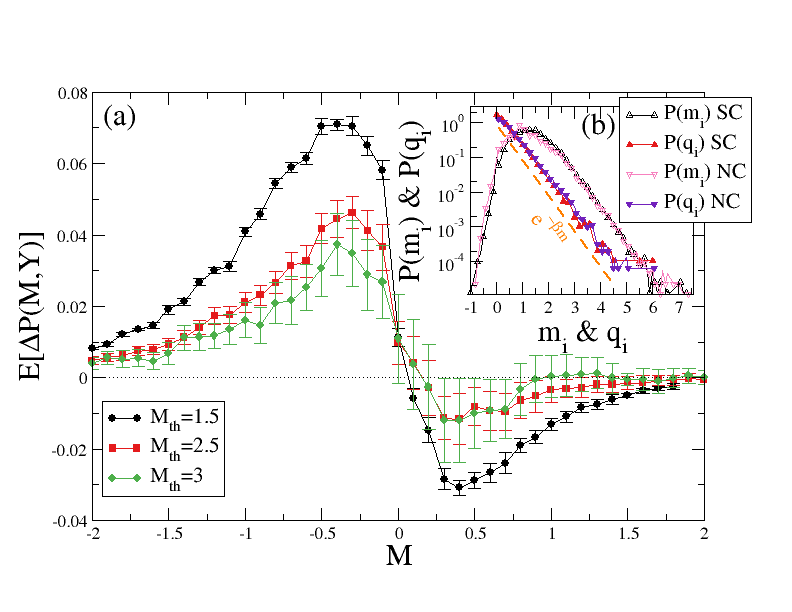
We then calculate the mean value , obtained by averaging over 1000 realizations of the reshuffled catalog . for SC is plotted in Fig.1a for the case where and km. The error bars represent twice the standard deviation . Values such as indicate that it is highly improbable for a catalog with uncorrelated magnitudes, such as , to produce the same probability of observing a given magnitude difference of the real catalog. Therefore, Fig.1a demonstrates that magnitudes in the instrumental catalog are correlated. In Fig.1a, we also examine the influence of a magnitude threshold on . By considering only earthquakes with magnitudes larger than and increasing , we observe a decrease in . This decrease can be interpreted as a signature that magnitude correlations are primarily a spurious effect of incompleteness, as increasing focuses on a catalog less affected by incompleteness. Nevertheless, the observation that even for , which exceeds the completeness magnitude estimated from the magnitude distribution (Fig.1b), suggests the persistence of genuine magnitude correlations beyond incompleteness. This scenario finds further support in the resilience of to variations in the quality of the seismic network [22] and is reinforced by laboratory experiments on rock fracture [33]. These experimental findings demonstrate the existence of magnitude clustering irrespective of loading protocols, rock types, and observable magnitude ranges.
Next, we will review these results in light of recent findings concerning positive magnitude difference statistics. We assume as null hypothesis that magnitudes are i.i.d variables which obey the Gutenberg-Richter (GR) law, for magnitudes larger than a lower limit . Although a precise estimate of is unavailable, it is reasonable to assume that takes on a very negative value [25]. Additionally, we assume that not all magnitudes are reported in the catalog due to detection issues. Therefore, the observed magnitude distribution is given by [41]
| (3) |
where is the completeness magnitude and is a detection function which is a monotonic increasing function of ranging from for to for . Essentially, earthquakes with magnitudes are undetected, while those with are always detected. A realistic functional form for is , with typical estimates placing in the range [46, 40, 41]. Eq.(3) is consistent with the magnitude distribution of instrumental catalogs (Fig.1b), which conforms to the GR law only for magnitudes , determined using the maximum curvature method [47], with for SC and for NC (Fig.1b).
Using Eq.(3) in Eq.(1), we obtain
| (4) | ||||
In the above equation, we explicitly use the notation to specify that the detection function must be evaluated under conditions where the previous earthquake has been identified and reported in the catalog. It is worth noticing that it is exactly this conditioned detection function that introduces correlations between the magnitudes and . Indeed, the same expression Eq.(4) holds for the probability , with instead of . This makes a fundamental difference since, by construction, is a random index, and therefore , independently of .
Accordingly, can be rewritten as
| (5) | ||||
The origin of magnitude correlations in the null hypothesis scenario originates from the difference of the two detection functions in the term between square brackets in Eq.(5). It is evident that, if , and is on average larger than . Indeed, if a previous earthquake has been detected, the probability to detect a subsequent larger one is larger compared to the case where no information about previously detected earthquakes is available. At the same time, imposing and by considering increasing values of , both detection functions and approach , and approaches zero. Accordingly, the behavior of in Fig.1a cannot exclude the null hypothesis scenario where magnitudes are i.i.d variables in the presence of detection problems.
We now explore the prediction of the null hypothesis on the magnitude difference , restricting to and . The parameter is chosen sufficiently small to ensure that earthquake pairs are close enough in space, guaranteeing similarity in the distance to the stations necessary for their identification. Under this condition, since the earthquake has been detected, it implies that , and therefore , for . Accordingly, from Eq.(4), for , , where is a constant given by . After derivation, we therefore obtain, for
| (6) |
showing that, even in the presence of detection problems, the distribution of magnitude differences follows an exponential GR decay for , independently of the previous seismic history. This behavior is observed in instrumental catalogs (Fig.1b), where we find that follows a pure exponential decay when is larger than a completeness threshold , for both SC and NC, consistent with Eq.(6), with the same value of the exponent ( in SC, in NC) extrapolated from the magnitude distribution (Eq.(3)) when (Fig.1b).
It is crucial to note that while detection issues introduce spurious correlations between and , positive magnitude differences remain unaffected by such detection problems. Consequently, when , the null hypothesis predicts no correlations between and . To delve deeper into this aspect, we select the subset of the catalog , denoted as , which contains only those earthquakes satisfying both constraints and , and therefore the -th element of the catalog will be the vector . From the catalog , we next obtain the catalog , whose elements are the vectors with . It is important to note that, in general, , and this equality only holds when and and are both smaller than . We also generate several reshuffled catalogs , where the -th element is the vector with , and is the index of a random earthquake in the catalog . We can define, , , and by simply replacing with and with in all the definitions from Eq.(1) to Eq.(4). Accordingly, from Eq.(5), under the null hypothesis Eq.(3), we obtain
| (7) | ||||
where and represent the conditioned and unconditioned probabilities, respectively, of detecting a magnitude difference . Correlations between and are induced by the term . Nevertheless, in contrast to where the information that event has been detected strongly constrains the detectability of , in this case, the information that the previous magnitude difference has been detected only weakly affects the probability to detect the next magnitude difference . In fact, we expect that , and is expected to be very small under the null-hypothesis scenario. In particular, by considering only magnitude differences , as increases, the detection probability also increases and approaches for . Consequently, we expect that presents small values when , and decreases as increases, vanishing when magnitude differences are detected with probability for .
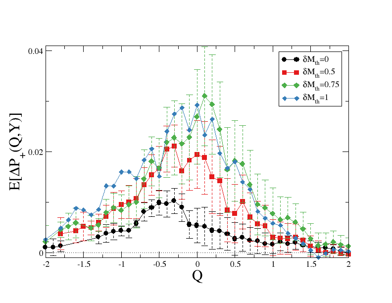
In the following we investigate the behavior of the mean value for the SC catalog. The main result is that exhibits a markedly different pattern (Fig.2) compared to the one predicted by the null hypothesis (Eq.(7)). While data for could be consitent with the null hypothesis Eq.(7), as evidenced by being only slightly larger than , the remarkable finding is that for larger values of , not only fails to decrease but rather increases. Particularly notable is that for , significantly surpassing , when the variables remain unaffected by detection issues (Fig.1b), the correlation between and becomes even more pronounced. The significant growth of as a function of is notable until , after which no substantial increase is observed up to . Results plotted in Fig.2 unequivocally demonstrate the presence of non-trivial correlations among magnitude differences. Consequently, the result derived from the null hypothesis of i.i.d. magnitudes, as expressed in Eq.(7), can be confidently dismissed.
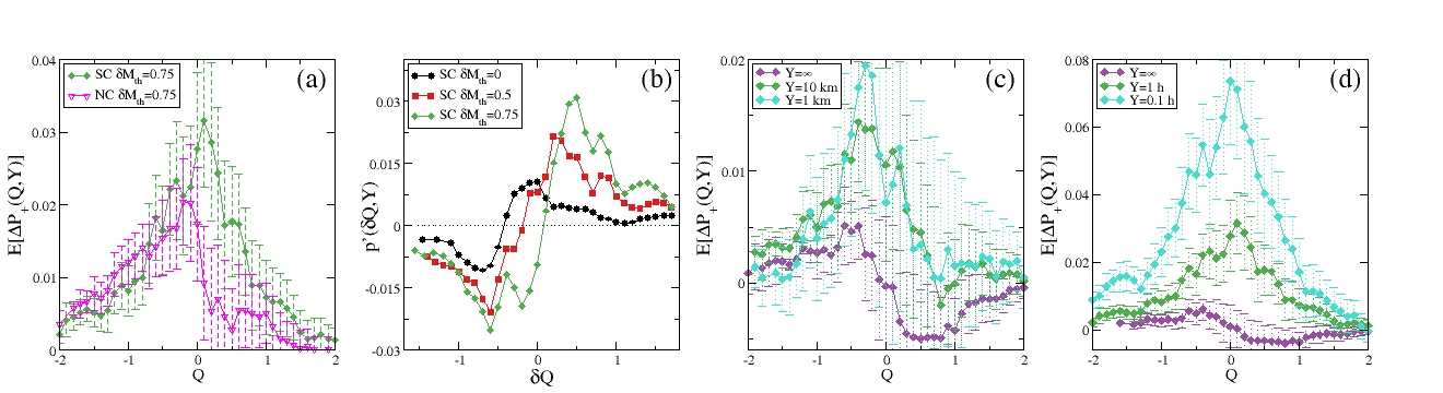
We note that the results presented in Fig.2 were derived by considering only earthquakes with epicentral distances smaller than km as elements of the catalog . Similar results were obtained for other choices of km. Additionally, comparable outcomes were observed when analyzing the NC catalog (Fig.3a). This suggests that correlations between magnitude differences appear to be a consistent characteristic of seismic catalogs, with patterns showing weak dependency on the geographic region.
In order to gain further insights into the mechanisms responsible for correlations between and , we examine the influence of on in Fig.3. Specifically, in Fig.3d, we consider and investigate decreasing values of , ranging from to hours. The results show that as decreases, imposing that earthquake pairs are closer in time, their correlation strengthens. In Fig.3c, we conduct a similar analysis but with , with decreasing from to km. Here, we observe that magnitude correlations become more pronounced as we transition from to km, but then stabilize, remaining roughly constant regardless of the specific value of . Consequently, magnitude correlations are stronger for earthquakes occurring closer in time, whereas they are only weakly affected by the spatial distance between earthquakes.
Further insights are provided by examining the derivative , which measures the difference in probability between the instrumental and reshuffled catalogs to observe . The results (Fig.3b) reveal that it is more probable for a magnitude difference to be followed by a larger one. Given that the inverse of the average value of coincides with [40], the origin of magnitude correlations could be linked to a decreasing value over time during aftershock sequences. This observation aligns with the pattern identified by Gulia & Wiemer [27] from their analysis of main-aftershock sequences. On the contrary, the scarcity of earthquakes preceding significant shocks poses a challenge in deriving conclusive insights from our analysis regarding the behavior of for foreshocks, and in comparing them with the predictive framework proposed in references [48, 49].
In summary, our findings unequivocally demonstrate the presence of non-trivial correlations between subsequent magnitude differences, suggesting potential modifications to be integrated into the ETAS model. One possible approach, as proposed by [29, 30], is to consider two distinct values for aftershocks, , depending on the magnitude of the triggering mainshock. Alternatively, a time-varying value during the aftershock sequence could also be implemented [50]. This novel research direction holds promise for extracting valuable insights from the intricate patterns of seismicity, ultimately enhancing our ability to forecast seismic events and advancing our understanding of the mechanisms governing earthquake triggering.
References
- Schorlemmer and Woessner [2008] D. Schorlemmer and J. Woessner, Bulletin of the Seismological Society of America 98, 2103 (2008).
- Mignan et al. [2011] A. Mignan, M. J. Werner, S. Wiemer, C.-C. Chen, and Y.-M. Wu, Bulletin of the Seismological Society of America 101, 1371 (2011).
- Mignan and Woessner [2012] A. Mignan and J. Woessner, Community Online Resource for Statistical Seismicity Analysis 10.5078/corssa-00180805 (2012).
- Kagan [2004] Y. Y. Kagan, Bulletin of the Seismological Society of America 94, 1207 (2004).
- Helmstetter et al. [2006] A. Helmstetter, Y. Y. Kagan, and D. D. Jackson, Bulletin of the Seismological Society of America 96, 90 (2006).
- Peng et al. [2007] Z. Peng, J. E. Vidale, M. Ishii, and A. Helmstetter, Journal of Geophysical Research: Solid Earth 112, n/a (2007), b03306.
- Lippiello et al. [2016] E. Lippiello, A. Cirillo, G. Godano, E. Papadimitriou, and V. Karakostas, Geophysical Research Letters 43, 6252 (2016), 2016GL069748.
- Hainzl [2016a] S. Hainzl, Journal of Geophysical Research: Solid Earth 121, 6499 (2016a), 2016JB013319.
- Hainzl [2016b] S. Hainzl, Seismological Research Letters 87, 337 (2016b).
- de Arcangelis et al. [2018] L. de Arcangelis, C. Godano, and E. Lippiello, Journal of Geophysical Research: Solid Earth 123, 5661 (2018).
- Petrillo et al. [2020] G. Petrillo, F. Landes, E. Lippiello, and A. Rosso, Nature Communications 11, 3010 (2020).
- Hainzl [2021] S. Hainzl, Bulletin of the Seismological Society of America 112, 494 (2021).
- Lippiello et al. [2019] E. Lippiello, C. Petrillo, C. Godano, A. Tramelli, E. Papadimitriou, and V. Karakostas, Nature Communications 10, 2953 (2019).
- Lippiello et al. [2007a] E. Lippiello, C. Godano, and L. de Arcangelis, Phys. Rev. Lett. 98, 098501 (2007a).
- Lippiello et al. [2007b] E. Lippiello, M. Bottiglieri, C. Godano, and L. de Arcangelis, Geophysical Research Letters 34, L23301 (2007b).
- Lippiello et al. [2008] E. Lippiello, L. de Arcangelis, and C. Godano, Phys. Rev. Lett. 100, 038501 (2008).
- Shcherbakov et al. [2005] R. Shcherbakov, G. Yakovlev, D. L. Turcotte, and J. B. Rundle, Phys. Rev. Lett. 95, 218501 (2005).
- Varotsos et al. [2005] P. A. Varotsos, N. V. Sarlis, H. K. Tanaka, and E. S. Skordas, Phys. Rev. E 72, 041103 (2005).
- Sarlis et al. [2010a] N. V. Sarlis, E. S. Skordas, and P. A. Varotsos, Phys. Rev. E 82, 021110 (2010a).
- Sarlis et al. [2010b] N. V. Sarlis, E. S. Skordas, and P. A. Varotsos, Phys. Rev. E 82, 021110 (2010b).
- Sarlis [2011] N. V. Sarlis, Phys. Rev. E 84, 022101 (2011).
- Lippiello et al. [2012] E. Lippiello, C. Godano, and L. de Arcangelis, Geophysical Research Letters 39, L05309 (2012).
- Davidsen and Green [2011] J. Davidsen and A. Green, Phys. Rev. Lett. 106, 108502 (2011).
- Nichols and Schoenberg [2014] K. Nichols and F. P. Schoenberg, Environmetrics 25, 143 (2014).
- de Arcangelis et al. [2016] L. de Arcangelis, C. Godano, J. R. Grasso, and E. Lippiello, Physics Reports 628, 1 (2016).
- Spassiani and Sebastiani [2016a] I. Spassiani and G. Sebastiani, Phys. Rev. E 93, 042134 (2016a).
- Gulia et al. [2018] L. Gulia, A. P. Rinaldi, T. Tormann, G. Vannucci, B. Enescu, and S. Wiemer, Geophysical Research Letters 45, 13,277 (2018).
- Ogata et al. [2018] Y. Ogata, K. Katsura, H. Tsuruoka, and N. Hirata, Seismological Research Letters 89, 1298 (2018).
- Nandan et al. [2019] S. Nandan, G. Ouillon, and D. Sornette, Journal of Geophysical Research: Solid Earth 124, 2762 (2019).
- Nandan et al. [2022] S. Nandan, G. Ouillon, and D. Sornette, Journal of Geophysical Research: Solid Earth 127, e2022JB024380 (2022), e2022JB024380 2022JB024380.
- Petrillo and Zhuang [2022] G. Petrillo and J. Zhuang, Sci Rep 12, 20683 (2022).
- Petrillo and Zhuang [2023] G. Petrillo and J. Zhuang, Phys. Rev. Lett. 131, 154101 (2023).
- Xiong et al. [2023] Q. Xiong, M. R. Brudzinski, D. Gossett, et al., Nature Communications 14, 2056 (2023).
- Taroni [2024] M. Taroni, Geophysical Journal International 236, 1596 (2024).
- Ogata [1985] Y. Ogata, Research Memo. Technical report Inst. Statist. Math., Tokyo. 288 (1985).
- Ogata [1988a] Y. Ogata, J. Amer. Statist. Assoc. 83, 9 – 27 (1988a).
- Ogata [1988b] Y. Ogata, Ann. Inst. Math.Statist. 50, 379–402 (1988b).
- Ogata [1989] Y. Ogata, Numerische Mathematik 55, 137 (1989).
- Spassiani and Sebastiani [2016b] I. Spassiani and G. Sebastiani, Journal of Geophysical Research: Solid Earth 121, 903 (2016b), 2015JB012398.
- van der Elst [2021] N. J. van der Elst, Journal of Geophysical Research: Solid Earth 126, e2020JB021027 (2021), e2020JB021027 2020JB021027.
- Lippiello and Petrillo [2024] E. Lippiello and G. Petrillo, Journal of Geophysical Research: Solid Earth 129, e2023JB027849 (2024), e2023JB027849 2023JB027849.
- van der Elst and Page [2023] N. J. van der Elst and M. T. Page, Journal of Geophysical Research: Solid Earth 128, e2023JB027089 (2023), e2023JB027089 2023JB027089.
- van der Elst [2023] N. J. van der Elst, AGU assembly (2023).
- Hauksson et al. [2012] E. Hauksson, W. Yang, and P. M. Shearer, Bulletin of the Seismological Society of America 102, 2239 (2012).
- Waldhauser and Schaff [2008] F. Waldhauser and D. P. Schaff, Journal of Geophysical Research: Solid Earth 113 (2008).
- Ogata and Katsura [1993] Y. Ogata and K. Katsura, Geophysical Journal International 113, 727 (1993).
- Woessner and Wiemer [2005] J. Woessner and S. Wiemer, Bulletin of the Seismological Society of America 95, 684 (2005).
- Gulia and Wiemer [2019] L. Gulia and S. Wiemer, Nature 574, 193 (2019).
- Gulia et al. [2020] L. Gulia, S. Wiemer, and G. Vannucci, Seismological Research Letters 91, 2828 (2020).
- Gulia et al. [2016] L. Gulia, T. Tormann, S. Wiemer, M. Herrmann, and S. Seif, Geophysical Research Letters 43, 1100 (2016).