An MRP Formulation for Supervised Learning:
Generalized Temporal Difference Learning Models

Abstract

In traditional statistical learning, data points are usually assumed to be independently and identically distributed (i.i.d.) following an unknown probability distribution. This paper presents a contrasting viewpoint, perceiving data points as interconnected and employing a Markov reward process (MRP) for data modeling. We reformulate the typical supervised learning as an on-policy policy evaluation problem within reinforcement learning (RL), introducing a generalized temporal difference (TD) learning algorithm as a resolution. Theoretically, our analysis draws connections between the solutions of linear TD learning and ordinary least squares (OLS). We also show that under specific conditions, particularly when noises are correlated, the TD’s solution proves to be a more effective estimator than OLS. Furthermore, we establish the convergence of our generalized TD algorithms under linear function approximation. Empirical studies verify our theoretical results, examine the vital design of our TD algorithm and show practical utility across various datasets, encompassing tasks such as regression and image classification with deep learning.

1 Introduction

The primary objective of statistical supervised learning (SL) is to learn the relationship between the features and the output (response) variable. To achieve this, generalized linear models (Nelder & Wedderburn, 1972; McCullagh & Nelder, 1989) are considered a generic algorithmic framework employed to derive objective functions. These models make specific assumptions regarding the conditional distribution of the response variable given input features, which can take forms such as Gaussian (resulting in ordinary least squares), Poisson (resulting in Poisson regression), or multinomial (resulting in logistic regression or multiclass softmax cross-entropy loss).

In recent years, reinforcement learning (RL), widely utilized in interactive learning settings, has witnessed a surge in popularity. This surge has attracted growing synergy between RL and SL, where each approach complements the other in various ways. In SL-assisted RL, the area of imitation learning (Hussein et al., 2017) may leverage expert data to regularize/speed up RL, while weakly supervised methods (Lee et al., 2020) have been adopted to constrain RL task spaces, and relabeling techniques contributed to goal-oriented policy learning (Ghosh et al., 2021). Ghugare et al. (2024) studied the generalization benefits of RL and proposed data augmentation from SL to improve RL.

Conversely, RL has also expanded its application into traditional SL domains. RL has proven effective in fine-tuning large language models (MacGlashan et al., 2017), aligning them with user preferences. Additionally, RL algorithms (Gupta et al., 2021) have been tailored for training neural networks (NNs), treating individual network nodes as RL agents. In the realm of imbalanced classification, RL-based control algorithms have been developed, where predictions correspond to actions, rewards are based on heuristic correctness criteria, and episodes conclude upon incorrect predictions within minority classes (Lin et al., 2020). Permative prediction (Perdomo et al., 2020) provides a theoretical framework that can deal with nonstationary data and it can be reframed within a RL context.

Existing approaches that propose a RL framework for solving SL problems often exhibit a heuristic nature. These approaches involve crafting specific formulations, including elements like agents, reward functions, action spaces, and termination conditions, based on intuitive reasoning tailored to particular tasks. Consequently, they lack generality, and their heuristic nature leaves theoretical assumptions, connections between optimal RL and SL solutions, and convergence properties unclear. To the best of our knowledge, it remains uncertain whether a unified and systematic RL formulation capable of modeling a wide range of conventional SL problems exists. Such a formulation should be agnostic to learning settings, including various tasks such as ordinary least squares regression, Poisson regression, binary or multi-class classification, etc.

In this study, we introduce a generic Markov process formulation for data generation, offering an alternative to the conventional i.i.d. data assumption in SL. Specifically, when faced with a SL dataset, we view the data points as originating from a Markov reward process (MRP) (Szepesvari, 2010). To accommodate a wide range of problems, such as Poisson regression, binary or multi-class classification, we introduce a generalized TD learning model in Section 3. Section 4 explores the relationship between the solutions obtained through TD learning and the original linear regression. Furthermore, we prove that under specific conditions with correlated noise, TD estimator is more efficient than the traditional ordinary least squares (OLS) estimator. We provide convergence result in Section 5 under linear function approximation. Our paper concludes with an empirical evaluation of our TD algorithm in Section 6, verifying our theoretical results, assessing its critical design choices and practical utility when integrated with a deep neural network across various tasks, achieving competitive results and, in some cases, improvements in generalization performance. We view our work as a step towards unifying diverse learning tasks from two pivotal domains within a single, coherent theoretical framework.

2 Background

This section provides a brief overview of the relevant concepts from statistical SL and RL settings, laying the groundwork for the rest of this paper.

2.1 Conventional Supervised Learning

In the context of statistical learning, we make the assumption that data points, in the form of $(\mathbf{\bm{x}},y)\in\mathcal{X}\times\mathcal{Y}$, are independently and identically distributed (i.i.d.) according to some unknown probability distribution $P$. The goal is to find the relationship between the feature $\mathbf{\bm{x}}$ and response variable $y$ given a training dataset $\mathcal{D}=\{(\mathbf{\bm{x}}_{i},y_{i})\}_{i=1}^{n}$.

In a simple linear function approximation case, a commonly seen algorithm is ordinary least squares (OLS) that optimizes squared error objective function

$$\min_{\mathbf{\bm{w}}}\ ||\mathbf{X}\mathbf{\bm{w}}-\mathbf{\bm{y}}||^{2}_{2}.$$ (1)

where $\mathbf{X}$ is the $n\times d$ feature matrix and $\mathbf{\bm{y}}$ is the corresponding $n$-dimensional training label vector, and the $\mathbf{\bm{w}}$ is the parameter vector we aim to optimize.

From a probabilistic perspective, this objective function can be derived by assuming $p(y|\mathbf{\bm{x}})$ follows a Gaussian distribution with mean $\mathbf{\bm{x}}^{\top}\mathbf{\bm{w}}$ and conducting maximum likelihood estimation (MLE) for $\mathbf{\bm{w}}$ with the training dataset. It is well known that $\mathbb{E}[Y|\mathbf{\bm{x}}]$ is the optimal predictor (Bishop, 2006). For many other choices of distribution $p(y|\mathbf{\bm{x}})$, generalized linear models (GLMs) (Nelder & Wedderburn, 1972) are commonly employed for estimating $\mathbb{E}[Y|\mathbf{\bm{x}}]$. This includes OLS, Poisson regression (Nelder, 1974) and logistic regression, etc.

An important concept in GLMs is the inverse link function, which we denoted as $f$, that establishes a connection between the linear prediction (also called the logit), and the conditional expectation: $\mathbb{E}[Y|\mathbf{\bm{x}}]=f(\mathbf{\bm{x}}^{\top}\mathbf{\bm{w}})$. For example, in logistic regression, the inverse link function is the sigmoid function. We later propose generalized TD learning models within the framework of RL that correspond to GLMs, enabling us to handle a wide range of data.

2.2 Reinforcement Learning

Reinforcement learning is often formulated within the Markov decision process (MDP) framework. An MDP can be represented as a tuple $(\mathcal{S},\mathcal{A},r,P,\gamma)$ (Puterman, 2014), where $\mathcal{S}$ is the state space, $\mathcal{A}$ is the action space, $r:{\mathcal{S}}\times\mathcal{A}\mapsto\mathbb{R}$ is the reward function, $P(\cdot|s,a)$ defines the transition probability, and $\gamma\in(0,1]$ is the discount factor. Given a policy $\pi:\mathcal{S}\times\mathcal{A}\rightarrow[0,1]$, the return at time step $t$ is $G_{t}=\sum_{i=0}^{\infty}\gamma^{i}r(S_{t+i},A_{t+i})$, and value of a state $s\in\mathcal{S}$ is the expected return starting from that state $v^{\pi}(s)=\mathbb{E}_{\pi}[G_{t}|S_{t}=s]$. In this work, we focus on the policy evaluation problem for a fixed policy, thus the MDP can be reduced to a Markov reward process (MRP) (Szepesvari, 2010) described by $(\mathcal{S},r^{\pi},P^{\pi},\gamma)$ where $r^{\pi}(s)\overset{\text{\tiny def}}{=}\sum_{a}\pi(a|s)r(s,a)$ and $P^{\pi}(s^{\prime}|s)\overset{\text{\tiny def}}{=}\sum_{a}\pi(a|s)P(s^{\prime}|s,a)$. When it is clear from the context, we will slightly abuse notations and ignore the superscript $\pi$.

In policy evaluation problem, the objective is to estimate the state value function of a fixed policy $\pi$ by using the trajectory $s_{0},r_{1},s_{1},r_{2},s_{2},...$ generated from $\pi$. Under linear function approximation, the value function is approximated by a parametrized function $v(s)\approx\mathbf{\bm{x}}(s)^{\top}\mathbf{\bm{w}}$ with parameters $\mathbf{\bm{w}}$ and some fixed feature mapping $\mathbf{\bm{x}}:\mathcal{S}\mapsto\mathbb{R}^{d}$ where $d$ is the feature dimension. Note that the state value satisfies the Bellman equation

$$v(s)=r(s)+\gamma\mathbb{E}_{S^{\prime}\sim P(\cdot|s)}[v(S^{\prime})].$$ (2)

One fundamental approach for the evaluation problem is the temporal difference (TD) learning (Sutton, 1988), which uses a sampled transition $s_{t},r_{t+1},s_{t+1}$ to update the parameters $\mathbf{\bm{w}}$ through stochastic fixed point iteration based on (2) with a step-size $\alpha>0$:

$$\mathbf{\bm{w}}\leftarrow\mathbf{\bm{w}}+\alpha(y_{t,td}-\mathbf{\bm{x}}(s_{t})^{\top}\mathbf{\bm{w}})\mathbf{\bm{x}}(s_{t}),$$ (3)

where $y_{t,td}\overset{\text{\tiny def}}{=}r_{t+1}+\gamma\mathbf{\bm{x}}(s_{t+1})^{\top}\mathbf{\bm{w}}$. To simplify notations and align concepts, we will use $\mathbf{\bm{x}}_{t}\overset{\text{\tiny def}}{=}\mathbf{\bm{x}}(s_{t})$. In linear function approximation setting, TD converges to the solution that solves the system $\mathbf{A}\mathbf{\bm{w}}=\mathbf{\bm{b}}$ (Bradtke & Barto, 1996; Tsitsiklis & Van Roy, 1997), where

$$\mathbf{A} =\mathbb{E}[\mathbf{\bm{x}}_{t}(\mathbf{\bm{x}}_{t}-\gamma\mathbf{\bm{x}}_{t+1})^{\top}]=\mathbf{X}^{\top}\mathbf{D}(\mathbf{I}-\gamma\mathbf{P})\mathbf{X},$$ (4)

$$\mathbf{\bm{b}} =\mathbb{E}[r_{t+1}\mathbf{\bm{x}}_{t}]=\mathbf{X}^{\top}\mathbf{D}\mathbf{\bm{r}}$$ (5)

with $\mathbf{X}\in\mathbb{R}^{|{\mathcal{S}}|\times d}$ being the feature matrix whose rows are the state features $\mathbf{\bm{x}}_{t}$, $\mathbf{D}\in\mathbb{R}^{|{\mathcal{S}}|\times|{\mathcal{S}}|}$ being the diagonal matrix with the stationary distribution $D(s_{t})$ on the diagonal, $\mathbf{P}\in\mathbb{R}^{|{\mathcal{S}}|\times|{\mathcal{S}}|}$ being the transition probability matrix (i.e., $\mathbf{P}_{ij}=P(s_{j}|s_{i})$) and $\mathbf{\bm{r}}\in\mathbb{R}^{|{\mathcal{S}}|}$ being the reward vector. To facilitate later discussions, we define $\mathbf{S}\overset{\text{\tiny def}}{=}\mathbf{D}(\mathbf{I}-\gamma\mathbf{P})$. Note that the matrix $\mathbf{A}$ is often invertible under mild conditions (Tsitsiklis & Van Roy, 1997).

3 MRP View and Generalized TD Learning

This section describes our MRP construction given the same dataset $\mathcal{D}=\{(\mathbf{\bm{x}}_{i},y_{i})\}_{i=1}^{n}$ and proposes our generalized TD learning algorithm to solve it. This approach is based on the belief that these data points originate from some MRP, rather than being i.i.d. generated.

Regression. We start by considering the basic regression setting with linear models before introducing our generalized TD algorithm. Table 1 summarizes how we can view concepts in the conventional SL from an RL perspective. The key is to treat the original training label as a state value that we are trying to learn, and then the reward function can be derived from the Bellman equation (2) as

$$r(s)=v(s)-\gamma\mathbb{E}_{S^{\prime}\sim P(\cdot|s)}[v(S^{\prime})].$$ (6)

We will discuss the choice of $P$ later. At each iteration (or time step in RL), the reward can be approximated using a stochastic example. For instance, assume that at iteration $t$ (i.e., time step in RL), we obtain an example $(\mathbf{\bm{x}}^{(t)}_{i},y^{(t)}_{i})$. We use superscripts and subscripts to denote that the $i$th training example is sampled at the $t$th time step. Then the next example $(\mathbf{\bm{x}}^{(t+1)}_{j},y^{(t+1)}_{j})$ is sampled according to $P(\cdot|\mathbf{\bm{x}}^{(t)}_{i})$ and the reward can be estimated as $r^{(t+1)}=y^{(t)}_{i}-\gamma y^{(t+1)}_{j}$ by approximating the expectation in Equation 6 with a stochastic example. As one might notice that, in a sequential setting the $t$ is monotonically increasing, hence we will simply use a simplified notation $(\mathbf{\bm{x}}_{t},y_{t})$ to denote the training example sampled at time step $t$.

SL Definitions	RL Definitions
Feature matrix $\mathbf{X}$	Feature matrix $\mathbf{X}$
Feature of the $i$th example $\mathbf{\bm{x}}_{i}$	The state feature $\mathbf{\bm{x}}(s_{i})=\mathbf{\bm{x}}_{i}$
Training target $y_{i}$ of $\mathbf{\bm{x}}_{i}$	The state value $v(s_{i})=y_{i}$

Table 1: How definitions in SL correspond to those in RL

We now summarize and compare the updating rules in conventional SL and in our TD algorithm under linear function approximation. At time step $t$, the conventional updating rule based on stochastic gradient descent (SGD) is

$$\mathbf{\bm{w}} \leftarrow\mathbf{\bm{w}}+\alpha(y_{t}-\mathbf{\bm{x}}_{t}^{\top}\mathbf{\bm{w}})\mathbf{\bm{x}}_{t},$$ (7)

while our TD updating rule is

$$\mathbf{\bm{w}} \leftarrow\mathbf{\bm{w}}+\alpha(y_{t,td}-\mathbf{\bm{x}}_{t}^{\top}\mathbf{\bm{w}})\mathbf{\bm{x}}_{t}$$ (8)

$$\text{where }\ y_{t,td} \overset{\text{\tiny def}}{=}r_{t+1}+\gamma{\color[rgb]{1,0,0}\widehat{y}_{t+1}}=y_{t}-\gamma y_{t+1}+\gamma{\color[rgb]{1,0,0}\mathbf{\bm{x}}_{t+1}^{\top}\mathbf{\bm{w}}}$$ (9)

and $\mathbf{\bm{x}}_{t+1}\sim P(\cdot|\mathbf{\bm{x}}_{t})$ with ground-truth label $y_{t+1}$. The critical difference is that TD uses a bootstrap, so it does not cancel the $\gamma y_{t+1}$ term from the reward when computing the TD training target $y_{t,td}$. By setting $\gamma=0$, one recovers the original supervised learning updating rule (7).

Generalized TD: An extension to general learning tasks. A natural question regarding TD is how to extend it to different types of data, such as those with counting, binary, or multiclass labels. Recall that in generalized linear models (GLMs), it is assumed that the output variable $y\in\mathcal{Y}$ follows an exponential family distribution. In addition, there exists an inverse link function $f$ that maps a linear prediction $z\overset{\text{\tiny def}}{=}\mathbf{\bm{w}}^{\top}\mathbf{\bm{x}}$ to the output/label space $\mathcal{Y}$ (i.e., $f(z)\in\mathcal{Y},\forall z\in\mathbb{R}$). Examples of GLMs include linear regression (where $y$ follows a Gaussian distribution, $f$ is the identity function and the loss is the squared loss) and logistic regression (where $y$ is Bernoulli, $f$ is the sigmoid function and the loss is the log loss). More generally, the output may be in higher dimensional space and both $z$ and $y$ will be vectors instead of scalars. As an example, multinomial regression uses the softmax function $f$ to convert a vector $\mathbf{\bm{z}}$ to another vector $\mathbf{\bm{y}}$ in the probability simplex. Interested readers can refer to Banerjee et al. (2005); Helmbold et al. (1999); McCullagh & Nelder (1989, Table 2.1) for more details. As per convention, we refer to $z$ as logit.

Back to TD algorithm, the significance of the logit $z$ is that it is naturally additive, which mirrors the additive nature of returns (cumulative sum of rewards) in RL. It also implies that one can add two linear predictions and the resultant $z=z_{1}+z_{2}$ can still be transformed to a valid output $f(z)\in\mathcal{Y}$. In contrast, adding two labels does not necessarily produce a valid label $y_{1}+y_{2}\notin\mathcal{Y}$. Therefore, the idea is to construct a bootstrapped target in the real line (logit space, or $z$-space)

$$\begin{split}z_{t,td}&\overset{\text{\tiny def}}{=}r_{t+1}+\gamma\widehat{z}_{t+1}=(z_{t}-\gamma z_{t+1})+\gamma\mathbf{\bm{x}}_{t+1}^{\top}\mathbf{\bm{w}}\end{split}$$

and then convert it back to the original label space to get the TD target $y_{t,td}=f(z_{t,td})$. In multiclass classification problems, we often use a one-hot vector to represent the original training target. For instance, in the case of MNIST, the target is a ten-dimensional one-hot vector. Consequently, the reward becomes a vector, with each component corresponding to a class. This can be interpreted as evaluating the policy under ten different reward functions in parallel and selecting the highest value for prediction.

Algorithm 1 provides the pseudo-code of our algorithm when using linear models. At time step $t$, the process begins by sampling the state $\mathbf{\bm{x}}_{t}$, and then we sample the next state according to the predefined $P$. The reward is computed as the difference in logits after converting the original labels $y_{t},y_{t+1}$ into the logit space with the link function. Subsequently TD bootstrap target is constructed in the logit space. Finally, the TD target is transformed back to the original label space before it is used to calculate the loss. Note that in standard regression is a special case where the (inverse) link function is simply the identity function, so it reduces to the standard update (7) with squared loss. In practice, we might need some smoothing parameter when the function $f^{-1}$ goes to infinity. For example, in binary classification, $\mathcal{Y}=\{0,1\}$ and the corresponding logits are $z=-\infty$ and $z=\infty$. To avoid this, we subtract/add some small value to the label before applying $f^{-1}$.

  Input: A dataset $\mathcal{D}$; randomly sample a data point $(\mathbf{\bm{x}}_{t},y_{t})\in\mathcal{D}$ as the starting point. (One can also use mini-batch starting points in NNs.)

  for $t=1,2,\ldots$ do

    Sample $\mathbf{\bm{x}}_{t+1}\sim P(\cdot|\mathbf{\bm{x}}_{t})$, let $y_{t+1}$ be its label

    $r_{t+1}\!=\!f^{-1}(y_{t})-\gamma f^{-1}(y_{t+1})$ // $f^{-1}$ converts to logits

    $z_{t,td}\!=\!r_{t+1}\!+\!\gamma\mathbf{\bm{x}}_{t+1}^{\top}\mathbf{\bm{w}}$

    $\mathbf{\bm{w}}\!\leftarrow\!\mathbf{\bm{w}}\!-\!\alpha\nabla l(f(\mathbf{\bm{x}}_{t}^{\top}\mathbf{\bm{w}}),f(z_{t,td}))$ // $f$ converts back to label

  end for

Algorithm 1 Generalized TD for SL

4 MRP v.s. i.i.d. for Supervised Learning

As our MRP formulation is fundamentally different from the traditional i.i.d. view, this section discusses the property of TD’s solution and its potential benefits in the linear setting and beyond. The section concludes with a discussion on the merits of adopting an MRP versus an i.i.d. perspective.

4.1 Connections between TD and OLS

The following proposition characterizes the connections between TD and OLS in the linear setting. Proof is in Appendix A.

Proposition 4.1.

[Connection between TD and OLS] When $\mathbf{D}$ has full support and $\mathbf{X}$ has linearly independent rows, TD and OLS have the same minimum norm solution. Moreover, any solution to the linear system $\mathbf{X}\mathbf{\bm{w}}=\mathbf{\bm{y}}$ must be also an solution to TD’s linear system $\mathbf{A}\mathbf{\bm{w}}=\mathbf{\bm{b}}$ as defined in Equation 5.

Remark. 1) The condition for equivalence holds when the transition probability matrix $\mathbf{P}$ is irreducible in overparametrization regime; 2) the min-norm property of TD’s solution is not new and was discussed by Xiao et al. (2022).

Empirical verification. Table 2 illustrates the distance between the closed-form solutions of our linear TD and OLS under various choices of the transition matrix by using a synthetic dataset (details are in Appendix B.1). Two key observations emerge: 1) As the feature dimension increases towards the overparameterization regime, both solutions become nearly indistinguishable, implying that designing $\mathbf{P}$ may be straightforward when employing a powerful model like NN. 2) Deficient choices for $\mathbf{P}$ with non-full support can pose issues and should be avoided. In practice, one might opt for a computationally and memory-efficient $\mathbf{P}$, such as a uniform constant matrix where every entry is set to $1/n$. Such a matrix is ergodic and, therefore, not deficient. We will delve deeper into the selection of $\mathbf{P}$ below.

	70	90	110	130
Random	0.027	0.075	$\leq 10^{-10}$	$\leq 10^{-10}$
Uniform	0.026	0.074	$\leq 10^{-10}$	$\leq 10^{-10}$
Distance (Far)	0.028	0.075	$\leq 10^{-10}$	$\leq 10^{-10}$
Distance (Close)	0.182	0.249	$\leq 10^{-10}$	$\leq 10^{-10}$
Deficient	0.035	0.172	0.782	0.650

Table 2: Distance between closed-form min-norm solutions of TD and OLS $\|\mathbf{\bm{w}}_{TD}-\mathbf{\bm{w}}_{LS}\|_{2}$. Input matrix $\mathbf{X}$ has normally distributed features with $n=100$ and various dimensions $d$. Results are average over $10$ runs. All standard errors are $\leq 0.02$ except the deficient case $\leq 0.25$. Details can be found in Appendix B.1.

4.2 Statistical Efficiency and Variance Analysis

A natural question is under what condition the TD solution is better than the OLS solution, especially given that they may find the same solution under specific conditions. Although the OLS estimator is known to be the best linear unbiased estimator (BLUE) under the i.i.d. assumption, our TD algorithm demonstrates the potential for a lower variance in settings with correlated noise, even when using a uniform transition matrix. Recall that conventional linear models assume $y_{i}=\mathbf{\bm{x}}_{i}^{\top}\mathbf{\bm{w}}^{*}+\epsilon_{i}$, where $\mathbf{\bm{w}}^{*}$ is the true parameters and $\epsilon_{i}$ is assumed to be independent noise. In contrast, under the MRP perspective, we consider the possibility of correlated noise. The following proposition shows when a TD estimator will be the most efficient one:

Proposition 4.2.

Suppose $\mathbf{A}$ is invertible and the error vector $\mathbf{\bm{\epsilon}}$ satisfies $\mathbb{E}[\mathbf{\bm{\epsilon}}|\mathbf{X}]=\mathbf{\bm{0}}$ and $\mathrm{Cov}[\mathbf{\bm{\epsilon}}|\mathbf{X}]=\mathbf{C}$. Then $\mathbb{E}[\mathbf{\bm{w}}_{TD}|\mathbf{X}]=\mathbf{\bm{w}}^{*}$ and the conditional covariance is

$$\mathrm{Cov}[\mathbf{\bm{w}}_{TD}|\mathbf{X}]=\mathbf{A}^{-1}\mathbf{X}^{\top}\mathbf{S}\mathbf{C}\mathbf{S}^{\top}\mathbf{X}(\mathbf{A}^{-1})^{\top}$$ (10)

Moreover, if $\mathbf{S}=\mathbf{S}^{\top}$, the TD estimator is the BLUE for problems with $\mathbf{C}=c\cdot\mathbf{S}^{-1},\forall c>0$.

Proof.

Recall from Equation 5 that $\mathbf{\bm{w}}_{TD}=\mathbf{A}^{-1}\mathbf{\bm{b}},\mathbf{\bm{b}}=\mathbf{X}^{\top}\mathbf{D}\mathbf{\bm{r}}$, and $\mathbf{\bm{r}}=(\mathbf{I}-\gamma\mathbf{P})\mathbf{\bm{y}}$. Therefore $\mathbf{\bm{w}}_{TD}\!-\!\mathbf{\bm{w}}^{*}$ equals

$$\mathbf{\bm{w}}_{TD}\!-\!\mathbf{\bm{w}}^{*}\! =\!\mathbf{A}^{-1}(\mathbf{\bm{b}}\!-\!\mathbf{A}\mathbf{\bm{w}}^{*})\!=\!\mathbf{A}^{-1}(\mathbf{X}^{\top}\mathbf{D}\mathbf{\bm{r}}\!-\!\mathbf{A}\mathbf{\bm{w}}^{*})$$ (11)

$$=\!\mathbf{A}^{-1}(\mathbf{X}^{\top}\!\mathbf{D}(\mathbf{I}\!-\!\gamma\mathbf{P})\mathbf{\bm{y}}\!-\!\mathbf{A}\mathbf{\bm{w}}^{*})\!$$ (12)

$$=\!\mathbf{A}^{-1}(\mathbf{X}^{\top}\!\mathbf{S}\mathbf{\bm{y}}\!-\!\mathbf{X}^{\top}\mathbf{S}\mathbf{X}\mathbf{\bm{w}}^{*})\!=\!\mathbf{A}^{-1}\mathbf{X}\mathbf{S}\mathbf{\bm{\epsilon}}$$ (13)

When $\mathbb{E}[\mathbf{\bm{\epsilon}}|\mathbf{X}]=\mathbf{\bm{0}}$, the conditional expectation of the above equation is zero. Thus $\mathbf{\bm{w}}_{TD}$ is conditionally unbiased and its conditional covariance is

$$\mathrm{Cov}[\mathbf{\bm{w}}_{TD}|\mathbf{X}] =\mathbf{A}^{-1}\mathbf{X}^{\top}\mathbf{S}\cdot\mathrm{Cov}[\mathbf{\bm{\epsilon}}|\mathbf{X}]\cdot\mathbf{S}^{\top}\mathbf{X}(\mathbf{A}^{-1})^{\top}$$ (14)

$$=\mathbf{A}^{-1}\mathbf{X}^{\top}\mathbf{S}\cdot\mathbf{C}\cdot\mathbf{S}^{\top}\mathbf{X}(\mathbf{A}^{-1})^{\top}$$ (15)

Finally, when $\mathbf{S}=\mathbf{S}^{\top}$ and $\mathbf{C}=c\cdot\mathbf{S}^{-1},c>0$, the TD estimator and its covariance become

$$\mathbf{\bm{w}}_{TD}\!=\!(\mathbf{X}^{\top}\mathbf{S}\mathbf{X})^{-1}\mathbf{X}\mathbf{S}\mathbf{\bm{y}},\ \mathrm{Cov}[\mathbf{\bm{w}}_{TD}|\mathbf{X}]\!=\!(c\mathbf{X}^{\top}\mathbf{S}\mathbf{X})^{-1}$$ (16)

By using the Cholesky decomposition $\mathbf{S}=\mathbf{L}\mathbf{L}^{\top}$, one can see that the TD estimator is equivalent to the OLS solution to a rescaled problem $\widetilde{\mathbf{\bm{y}}}=\widetilde{\mathbf{X}}\mathbf{\bm{w}}+\widetilde{\mathbf{\bm{\epsilon}}}$ where

$$\widetilde{\mathbf{\bm{y}}}=\mathbf{L}\mathbf{\bm{y}}\qquad\widetilde{\mathbf{X}}=\mathbf{L}\mathbf{X}\qquad\widetilde{\mathbf{\bm{\epsilon}}}=\mathbf{L}\mathbf{\bm{\epsilon}}$$ (17)

Here $\mathrm{Cov}[\widetilde{\mathbf{\bm{\epsilon}}}|\mathbf{X}]=\mathbf{L}\mathbf{C}\mathbf{L}^{\top}=c\mathbf{I}$ so the TD estimator is the OLS solution to this problem and thus is the BLUE. ∎

Remark 1. This proposition identifies a situation in which our TD estimator outperforms other estimators, OLS included, in terms of efficiency. The condition $\mathbf{S}=\mathbf{S}^{\top}$ is needed so that there exists a corresponding symmetric covariance matrix $\mathbf{C}$ for the data. This condition implies that $\mathbf{D}\mathbf{P}=\mathbf{P}^{\top}\mathbf{D}$, or $D(s_{i})P(s_{j}|s_{i})=D(s_{j})P(s_{i}|s_{j})$, which means the Markov chain is reversible (i.e., detailed balance). Also note that $\mathbf{S},\mathbf{A}$ are invertible under mild conditions (e.g., ergodic Markov chain). In such cases, the TD estimator is also the generalized least squares (GLS) estimator (Aitken, 1936; Kariya & Kurata, 2004). In practice, covariance matrix may be unknown and needs to be estimated, thereby resorting to Feasible GLS (FGLS) (Baltagi, 2008). However, estimating a covariance matrix is nontrivial as demonstrated in Section 6. It should be emphasized that GLS/FGLS methods do not naturally support incremental learning, nor is it readily adaptable to deep learning models.

Remark 2. TD’s application can be made more flexible by introducing emphatic TD (Sutton et al., 2016), which allows for transition-based $\gamma$ and interest weighting, thereby offering more flexibility in designing the matrix $\mathbf{S}$. We leave such extension as a future work. It is important to note that the variance of the current TD estimator does not have an interpretable closed form expression under more general $\mathbf{S}$ or when extending beyond the linear case. Below, we provide a more general perspective to understand the benefits of TD in terms of variance reduction. The basic idea is that when the ground truth target variables of consecutive time steps are positively correlated, the TD target benefits from a reduction in variance.

Proposition 4.3.

Assume the estimated next-state value $\widehat{y}_{t+1}$ satisfies $\widehat{y}_{t+1}=\mathbb{E}[y_{t+1}]+\epsilon$ where $\epsilon$ is some independent noise with zero mean and standard deviation $\sigma_{\epsilon}$. Let $\sigma_{t}$ be the standard deviation of $y_{t}$ and $\rho_{t,t+1}$ be the Pearson correlation coefficient between $y_{t}$ and $y_{t+1}$. If $\rho_{t,t+1}\geq\frac{\gamma^{2}\sigma_{t+1}^{2}+\sigma_{\epsilon}^{2}}{2\gamma\sigma_{t}\sigma_{t+1}}$, then $\mathrm{Var}(y_{t,td})\leq\mathrm{Var}(y_{t})$.

Proof.

We rewrite the TD target (9) as

$$y_{t,td}\! =\!(y_{t}\!-\!\gamma y_{t+1})\!+\!\gamma\mathbb{E}[y_{t+1}]\!+\!\epsilon\!=\!y_{t}\!-\!\gamma(y_{t+1}\!-\!\mathbb{E}[y_{t+1}])\!+\!\epsilon$$

This means we can treat $y_{t+1}$ as a control variate and the variance of this estimate is

$$\mathrm{Var}(y_{t,td})\! =\!\mathrm{Var}(y_{t})\!+\!\gamma^{2}\mathrm{Var}(y_{t+1})\!-\!2\gamma\mathrm{Cov}(y_{t},y_{t+1})\!+\!\mathrm{Var}(\epsilon)$$

$$=\sigma_{t}^{2}+\gamma^{2}\sigma_{t+1}^{2}-2\gamma\rho_{t,t+1}\sigma_{t}\sigma_{t+1}+\sigma_{\epsilon}^{2}$$

Plugging into the condition on $\rho_{t,t+1}$ would yield $\mathrm{Var}(y_{t,td})\leq\mathrm{Var}(y_{t})$. ∎

Remark. To better interpret the result, we can consider $\sigma_{t}=\sigma_{t+1}$, then the variance of TD’s target is simplified to

$$\mathrm{Var}(y_{t,td})=\sigma_{t}^{2}+\gamma^{2}\sigma_{t}^{2}-2\gamma\rho_{t,t+1}\sigma_{t}^{2}+\sigma_{\epsilon}^{2},$$ (18)

which achieves its lowest value, $(1-\rho^{2}_{t,t+1})\sigma_{t}^{2}+\sigma_{\epsilon}^{2}$ when $\gamma=\rho_{t,t+1}$. This suggests that the stronger correlation it is, the more (i.e. a larger $\gamma$) we might rely on the bootstrap term to reduce variance, coinciding with our intuition.

Empirical verification. Here we verify that when the outputs are indeed positively correlated, our method can generalize better than OLS. To this end, we construct a Gaussian process where the covariance matrix has ones on the diagonal and $\rho\in(0,1)$ on the off-diagonals. We compare the test losses between the OLS solution and our TD solution when using different $\rho$ values. Figure 1(a) shows that as the outputs become more positively correlated, TD generalizes better than OLS. Additionally, we test on a different setting where points within the same cluster are positively correlated and otherwise uncorrelated, and check if transitioning to correlated points as specified by $\mathbf{P}$ can help. Figure 1(b) shows that as $\mathbf{P}$ aligns more with the correlation, TD performs better. Detail setup can be found in Appendix B.2.

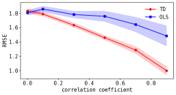
(a) RMSE v.s. correlation

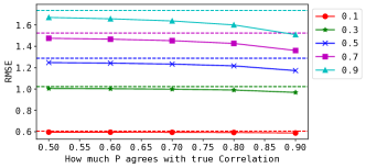
(b) RMSE v.s. P agreement

Figure 1: (a) shows when employing a uniform transition probability matrix $\mathbf{P}$, TD increasingly outperforms OLS as the correlation increases. (b) illustrates that under different levels of correlation, as indicated by various colors, TD (solid lines) increasingly outperforms OLS (dashed lines) when the transition probability matrix $\mathbf{P}$ more closely aligns with the correlation strength. $\mathbf{P}$ is designed such that a higher transition probability is assigned between two points when their outputs exhibits a stronger positive correlation.

Practical choices: MRP view v.s. i.i.d. view. In machine learning, the selection of algorithms often depends on whether their underlying assumptions align with the ground truth of the data – a factor that is fundamentally unknowable. Thus, the decision often boils down to personal belief – whether to treat the data as MRP or i.i.d. It is noteworthy that the TD algorithm demonstrates greater generality as it: 1) accommodates the solution of the linear system as demonstrated in Proposition 4.1 and is equivalent to OLS under certain conditions; 2) offers a straightforward approach to setting the discount factor to zero, effectively reducing the bootstrap target to the original SL training target.

The theoretical and empirical results from this section suggest: 1) in the absence of prior knowledge, adopting TD with small $\gamma$ values and a uniform $\mathbf{P}$ could be beneficial for computational and memory efficiency; if the ground truth suggests that the data points are positively correlated, this approach might yield a performance gain; 2) when it is known that two points are positively or negatively correlated, one might enhance variance reduction by strategically choosing to transition from one point to another or avoid such transitions.

5 Convergence Analysis

In this section, we present convergence results for our generalized TD algorithm (Algorithm 1) under both the expected updating rule and the sample-based updating rule. Detailed proofs are provided in Section A.2.

Here we show the finite-time convergence when using our TD(0) updates with linear function approximation. We primarily follow the convergence framework presented in (Bhandari et al., 2018), making nontrivial adaptations due to the presence of the inverse link function. Let $z(s)=\mathbf{\bm{x}}(s)^{\top}\mathbf{\bm{w}}$, or $z=\mathbf{\bm{x}}^{\top}\mathbf{\bm{w}}$ for conciseness.

Assumption 5.1 (Feature regularity).

$\forall s\in{\mathcal{S}},\|\mathbf{\bm{x}}(s)\|_{2}\leq 1$ and the steady-state covariance matrix $\mathbf{\Sigma}\overset{\text{\tiny def}}{=}D(s)\mathbf{\bm{x}}(s)\mathbf{\bm{x}}(s)^{\top}$ has full rank.

5.1 is a typical assumption necessary for the existence of the fixed point when there is no transform function (Tsitsiklis & Van Roy, 1997).

Assumption 5.2.

The inverse link function $f:\mathbb{R}\mapsto\mathcal{Y}$ is continuous, invertible and strictly increasing. Moreover, it has bounded derivative $f^{\prime}$ on any bounded domain.

5.2 is satisfied for those inverse link functions commonly used in GLMs, including but not limit to identity function (linear regression), exponential function (Poisson regression), and sigmoid function (logistic regression) (McCullagh & Nelder, 1989, Table 2.1). We can consider training in a sufficiently large compact $\mathcal{W}\subset\mathbb{R}^{d}$ such that the fixed point $\mathbf{\bm{w}}^{*}\in\mathcal{W}$. Then the following lemma holds.

Lemma 5.3.

Under 5.1, 5.2 and $\mathbf{\bm{w}}\in\mathcal{W}$, there exists $L\geq 1$ such that $\forall s_{1},s_{2}\in{\mathcal{S}}$ with $z_{1}=\mathbf{\bm{x}}(s_{1})^{\top}\mathbf{\bm{w}},z_{2}=\mathbf{\bm{x}}(s_{2})^{\top}\mathbf{\bm{w}}$,

$$\frac{1}{L}|z_{1}-z_{2}|\leq|f(z_{1})-f(z_{2})|\leq L|z_{1}-z_{2}|.$$ (19)

The next assumption is necessary later to ensure that the step size is positive.

Assumption 5.4 (Bounded discount).

The discount factor satisfies $\gamma<\frac{1}{L^{2}}$ for the $L$ in Lemma 5.3.

Convergence under expected update. The expected update rule is given by

$$\mathbf{\bm{w}}_{t+1}=\mathbf{\bm{w}}_{t}+\alpha\overline{g}(\mathbf{\bm{w}}_{t})\quad\text{ with }\quad\overline{g}(\mathbf{\bm{w}}_{t})\overset{\text{\tiny def}}{=}\mathbb{E}[(y_{td}-y)\mathbf{\bm{x}}]$$ (20)

where $y\overset{\text{\tiny def}}{=}f(z),y_{td}\overset{\text{\tiny def}}{=}f(r+\gamma\mathbf{\bm{x}}^{\prime\top}\mathbf{\bm{w}}_{t})$ and $\mathbf{\bm{x}}^{\prime}\overset{\text{\tiny def}}{=}\mathbf{\bm{x}}(s^{\prime})$.

One can expand the distance from $\mathbf{\bm{w}}_{t+1}$ to $\mathbf{\bm{w}}^{*}$ as

$$\|\mathbf{\bm{w}}^{*}\!\!\!-\!\mathbf{\bm{w}}_{t+1}\!\|_{2}^{2}\!=\!\|\mathbf{\bm{w}}^{*}\!\!\!-\!\mathbf{\bm{w}}_{t}\|_{2}^{2}\!-\!2\alpha(\mathbf{\bm{w}}^{*}\!\!\!-\!\mathbf{\bm{w}}_{t})^{\top}\!\overline{g}(\mathbf{\bm{w}}_{t})\!+\!\alpha^{2}\!\|\overline{g}(\mathbf{\bm{w}}_{t})\|_{2}^{2}$$

The common strategy is to make sure that the second term can outweigh the third term on the RHS so that $\mathbf{\bm{w}}_{t+1}$ can get closer to $\mathbf{\bm{w}}^{*}$ than $\mathbf{\bm{w}}_{t}$ in each iteration. This can be achieved by choosing an appropriate step size as shown below:

Theorem 5.5.

[Convergence with Expected Update] Under 5.1-5.4, consider the sequence $(\mathbf{\bm{w}}_{0},\mathbf{\bm{w}}_{1},\cdots)$ satisfying Equation 20. Let $\overline{\mathbf{\bm{w}}}_{T}\overset{\text{\tiny def}}{=}\frac{1}{T}\sum_{t=0}^{T-1}\mathbf{\bm{w}}_{t}$, $\overline{z}_{T}=\mathbf{\bm{x}}^{\top}\overline{\mathbf{\bm{w}}}_{T}$ and $z^{*}=\mathbf{\bm{x}}^{\top}\mathbf{\bm{w}}^{*}$. By choosing $\alpha=\frac{1-\gamma L^{2}}{4L^{3}}>0$, we have

$$\mathbb{E}\left[(z^{*}\!-\!\overline{z}_{T})^{2}\right] \!\leq\!\left(\frac{2L^{2}}{1\!-\!\gamma L^{2}}\!\right)^{2}\frac{\|\mathbf{\bm{w}}^{*}-\mathbf{\bm{w}}_{0}\|_{2}^{2}}{T}$$ (21)

$$\|\mathbf{\bm{w}}^{*}\!-\!\mathbf{\bm{w}}_{T}\|_{2}^{2} \leq\exp\left(-T\omega\left(\!\frac{1\!-\!\gamma L^{2}}{2L^{2}}\right)^{2}\!\right)\|\mathbf{\bm{w}}^{*}\!-\!\mathbf{\bm{w}}_{0}\|_{2}^{2}$$ (22)

Equation 21 shows that in expectation, the average prediction converges to the true value in the $z$-space, while Equation 22 shows that the last iterate converges to the fixed point exponentially fast when using expected update. In practice, we prefer sample-based updates is preferred and we discuss its convergence next.

Convergence under sample-based update. Below theorem shows the convergence under i.i.d. sample setting. Suppose $s_{t}$ is sampled from the stationary distribution $D(s)$ and $s_{t+1}\sim P(\cdot|s_{t})$. For conciseness, let $\mathbf{\bm{x}}_{t}\overset{\text{\tiny def}}{=}\mathbf{\bm{x}}(s_{t})$ and $\mathbf{\bm{x}}_{t+1}\overset{\text{\tiny def}}{=}\mathbf{\bm{x}}(s_{t+1})$. Then the sample-based update rule is

$$\mathbf{\bm{w}}_{t+1}=\mathbf{\bm{w}}_{t}+\alpha_{t}g_{t}(\mathbf{\bm{w}}_{t})\text{ with }g_{t}(\mathbf{\bm{w}}_{t})\overset{\text{\tiny def}}{=}(y_{t,td}-y_{t})\mathbf{\bm{x}}_{t}$$ (23)

where $y_{t}\!\overset{\text{\tiny def}}{=}\!f(\mathbf{\bm{x}}_{t}^{\top}\mathbf{\bm{w}}_{t}),y_{t,td}\!\overset{\text{\tiny def}}{=}f(z_{t,td})\!=\!f(r_{t+1}\!+\!\gamma\mathbf{\bm{x}}_{t+1}^{\top}\mathbf{\bm{w}}_{t})$.

The following theorem shows the convergence when using i.i.d. sample for the update:

Theorem 5.6.

[Convergence with Sampled-based Update] Under 5.1-5.4, with sample-based update Equation 23, let $\sigma^{2}=\mathbb{E}[\|g_{t}(\mathbf{\bm{w}}^{*})\|_{2}^{2}]$, $\overline{\mathbf{\bm{w}}}_{T}\overset{\text{\tiny def}}{=}\frac{1}{T}\sum_{t=0}^{T-1}\mathbf{\bm{w}}_{t}$, $\overline{z}_{T}=\mathbf{\bm{x}}^{\top}\overline{\mathbf{\bm{w}}}_{T}$ and $z^{*}=\mathbf{\bm{x}}^{\top}\mathbf{\bm{w}}^{*}$. For $T\geq\frac{64L^{6}}{(1-\gamma L^{2})^{2}}$ and a constant step size $\alpha_{t}=1/\sqrt{T},\forall t$, we have

$$\mathbb{E}\left[(z^{*}-\overline{z}_{T})^{2}\right]\leq\frac{L\left(\|\mathbf{\bm{w}}^{*}-\mathbf{\bm{w}}_{0}\|_{2}^{2}+2\sigma^{2}\right)}{\sqrt{T}(1-\gamma L^{2})}.$$ (24)

This shows that the generalized TD update converges even when using sample-based update. Not surprisingly, it is slower than using the expected update (21).

6 Empirical Studies

This section aims at: 1) validating whether the theoretical results of variance analysis still apply in real-world datasets in both linear and NN setting; 2) investigating the practical utility of our algorithm in a standard learning setting. Our conclusions are as follows: 1) TD learning performs in line with our theoretical expectations in either linear or neural network settings with correlated noise; 2) in a standard SL setting, TD demonstrates performance on par with traditional SL methods. Results on additional data and any missing details are in Appendix C.

Setup overview. For regression with real targets, we adopt the popular dataset execution time (Paredes & Ballester-Ripoll, 2018). For image classification, we use the popular MNIST (LeCun et al., 2010), Fashion-MNIST (Xiao et al., 2017), Cifar10 and Cifar100 (Krizhevsky, 2009) datasets. Additional results on other popular datasets (e.g. house price, bike rental, weather, insurance) are in  Appendix C. In TD algorithms, unless otherwise specified, we use a fixed transition probability matrix with all entries set to $1/n$, which is memory and computation efficient, and simplifies sampling processes.

Baselines and naming rules. TDReg: our TD approach, with its direct competitor being Reg (conventional $l_{2}$ regression). Reg-WP: Utilizes the same probability transition matrix as TDReg but does not employ bootstrap targets. This baseline can be used to assess the effect of bootstrap and transition probability matrix.

Linear setting with correlated noise. As outlined in Section 4.2, we anticipate that in scenarios where the target noise exhibits positive correlation, TD learning should leverage the advantages of using a transition matrix. When this matrix transitions between points with correlated noise, the TD target counterbalances the noise, thereby reducing variance. As depicted in Figure 2, we observe that with an increasing correlation coefficient (indicative of progressively positively correlated noise), TD consistently shows improved generalization performance towards the underlying best baseline.

In these figures, alongside TD and OLS, we include two baselines known for their efficacy in handling correlated noise: generalized least squares (GLS) and feasible GLS (FGLS) (Aitken, 1936). It is noteworthy that GLS operates under the assumption that the covariance of noise generation is fully known, aiming to approximate the underlying optimal estimator $\mathbf{\bm{w}}^{*}$. FGLS has two procedures: estimate the covariance matrix followed by applying this estimation to resolve the linear system. Please refer to Section C.2 for details.

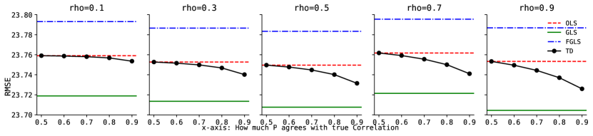
Figure 2: Test root mean squared error (RMSE) versus different values of $P$ on exec time dataset. From left to right, the noise correlation coefficient increases ($\rho\in\{0.1,0.3,0.5,0.7,0.9\}$). Each plot’s x-axis represents the degree of alignment between the transition matrix $P$ and the true covariance matrix that generates the noise. As $P$ aligns better – implying a higher likelihood of data points with positively correlated noise transitioning from one to another – the solution of TD increasingly approximates the $\mathbf{\bm{w}}^{*}$. Furthermore, as the correlation among the data intensifies, one can see larger gap between TD and OLS/FGLS.

Deep learning: regression with correlated noise. Similar to the previous experiment, we introduced noise to the original training target using a GP and opted for a uniform transition matrix. The results, depicted in Figure 3, reveal two key observations: 1) As the noise level increases, the performance advantage of TD over the baselines becomes more pronounced; 2) The baseline Reg-WP performs just as poorly as conventional Reg, underscoring the pivotal role of the TD target in achieving performance gains. Additionally, it was observed that all algorithms select the same optimal learning rate even when smaller learning rates are available, and TD consistently chooses a large $\gamma=0.95$. This implies that TD’s stable performance is attributed NOT to the choice of a smaller learning rate, but rather to the bootstrap target. Additional results are in Figure 6.

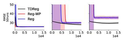
Figure 3: Learning curves on execute time dataset. From left to right, the noise defined as $c\times\epsilon$ where $\epsilon$ is noise generated by GP process and $c\in\{10,20,30\}$. Due to the addition of large-scale noise, Reg-WP and Reg exhibit high instability during the early learning stages and ultimately converge to a suboptimal solution compared to our TD (in black line) approach.

Deep learning: standard problems. We found that there is no clear gain/lose with TD’s bootstrap target in either regression (Table 3) or image classification tasks (Table 4). For image datasets, we employed a convolutional neural network (CNN) architecture and ResNN$18$ (He et al., 2016) to demonstrate TD’s practical utility.

	TD-Reg	Reg-WP	Reg
house	3.384 $\pm$ 0.21	3.355 $\pm$ 0.23	3.319 $\pm$ 0.16
exectime	23.763 $\pm$ 0.38	23.794 $\pm$ 0.36	23.87 $\pm$ 0.36
bikeshare	40.656 $\pm$ 0.77	40.904 $\pm$ 0.36	40.497 $\pm$ 0.45

Table 3: Test root mean squared error (RMSE) with standard error. The results have been smoothed using a 5-point window before averaging over 5 runs.

	TD-Classify	Classify
mnist	$99.06\%$	$99.00\%$
mnistfashion	$89.10\%$	$88.96\%$
cifar10	$67.42\%$	$67.13\%$
cifar100	$31.55\%$	$31.21\%$
cifar10(Resnn18)	$84.28\%$	$84.37\%$
cifar100(Resnn18)	$56.42\%$	$56.36\%$

Table 4: Image classification test accuracy. The results are smoothed over $10$ evaluations before averaging over $3$ random seeds. The standard errors are small with no definitive advantage observed for either algorithm.

We then further study the hyperparameter sensitivity in  Figure 4. With NNs, TD can pose challenges due to the interplay of two additional hyperparameters: $\gamma$ and the target NN moving rate $\tau$ (Mnih et al., 2015). Optimizing these hyperparameters can often be computationally expensive. Therefore, we investigate their impact on performance by varying $\gamma,\tau$. We find that selecting appropriate parameters tends to be relatively straightforward. Figure 4 displays the testing performance across various parameter settings. It is evident that performance does not vary significantly across settings, indicating that only one hyperparameter or a very small range of hyperparameters needs to be considered during the hyperparameter sweep. It should be noted that Figure 4 also illustrates the sensitivity analysis when employing three intuitive types of transition matrices that do not require prior knowledge. It appears that there is no clear gain/lose with these choices in a standard task. We refer readers to Appendix C.5 for details.

(a) Bikeshare

(b) ExecutionTime

(c) House

Figure 4: Sensitivity to hyperparameter settings. We show test RMSE with error bars while sweeping over discount rate $\gamma\in\{0.1,0.2,0.4,0.9\}$, target NN moving rate $\tau\in\{0.001,0.01,0.1,0.2,0.4,0.9\}$, and three types of transition probability. $\gamma$ hurts when it goes to the largest value on bikeshare, and it is likely because the exponential term in Poisson regression needs a unusually small learning rate. When generating curves for $\tau$ and $\gamma$, we maintain $P_{\text{type}}$ as a simple uniform constant.

7 Conclusion

This paper introduces a universal framework that transforms traditional SL problems into RL problems, alongside proposing a generalized TD algorithm. We highlight a specific set of problems for which such algorithms are apt and the potential variance reduction benefits of TD. Additionally, we establish the convergence properties of our algorithm. Empirical evidence, encompassing both linear and deep learning contexts, is provided to validate our theoretical findings and to evaluate the algorithm’s design and practical applicability. This research represents a foundational step towards bridging classic SL and RL paradigms. Our MRP formulation essentially offers a perspective that links various data points, corresponding to an interconnected worldview.

Future work and limitations. Our current analysis of covariance does not account for the potential advantages in scenarios where the matrix $\mathbf{S}$ is non-symmetric. This gap is due to both the absence of relevant literature and the lack of interpretable closed-form expressions. It is plausible that specific types of transition matrix designs could be advantageous in certain applications – particularly when they align with the underlying data assumptions. Additionally, our discussion does not encompass the potential benefits of incorporating more recent TD algorithms such as emphatic TD (Sutton et al., 2016), gradient TD (Maei, 2011), or accelerated TD (Pan et al., 2017b, a), which have been shown to enhance stability or convergence. Furthermore, it would be more intriguing to explore the utility of the probability transition matrix in a broader context, such as transfer learning, domain adaptation, or continual learning settings. Lastly, extending our approach to test its effectiveness with more modern NNs, such as transformers, could be of significant interest to a broader community.

Impact Statement

This paper presents work whose goal is to advance the field of machine learning. There may be potential societal consequences of our work, none of which we feel must be specifically highlighted here.

Table of Contents

1. Appendix A provides the proof of Proposition 4.1 and convergence proof details.

2. Appendix B provides implementation details on synthetic datasets from Section 4.1 and Section 4.2.

3. Appendix C provides implementation details and additional results on those real-world datasets:

   • Linear regression ( Section C.2),

   • Regression with Neural Networks (NNs) ( Section C.3),

   • Binary classification with NNs ( Section C.4),

   • Implementation details of different heuristically designed $\mathbf{P}$ are in Section C.5.

Appendix A Proofs

A.1 Proof for Proposition 4.1

See 4.1

Proof.

In our TD formulation, the reward is $\mathbf{\bm{r}}=(\mathbf{I}-\gamma\mathbf{P})\mathbf{\bm{y}}$. With $\mathbf{S}=\mathbf{D}(\mathbf{I}-\gamma\mathbf{P})$, we have $\mathbf{A}=\mathbf{X}^{\top}\mathbf{S}\mathbf{X}$, and $\mathbf{\bm{b}}=\mathbf{X}^{\top}\mathbf{S}\mathbf{\bm{y}}$. To verify the first claim, define The min-norm solutions found by TD and OLS are respectively $\mathbf{\bm{w}}_{TD}=\mathbf{A}^{\dagger}\mathbf{\bm{b}}$, and $\mathbf{\bm{w}}_{LS}=\mathbf{X}^{\dagger}\mathbf{\bm{y}}$, where

$$\mathbf{\bm{w}}_{TD}=\mathbf{A}^{\dagger}\mathbf{\bm{b}}=(\mathbf{X}^{\top}\mathbf{S}\mathbf{X})^{\dagger}\cdot\mathbf{X}^{\top}\mathbf{S}\mathbf{\bm{y}}.$$ (25)

When $\mathbf{D}$ has full support, $\mathbf{S}$ is invertible (thus has linearly independent rows/columns). Additionally, $\mathbf{X}$ has linearly independent rows so $(\mathbf{X}^{\top}\mathbf{S}\mathbf{X})^{\dagger}=\mathbf{X}^{\dagger}\mathbf{S}^{-1}(\mathbf{X}^{\top})^{\dagger}$ (Greville, 1966, Thm.3) and the TD solution becomes

$$\mathbf{\bm{w}}_{TD}=\mathbf{A}^{\dagger}\mathbf{\bm{b}}=\mathbf{X}^{\dagger}\mathbf{S}^{-1}(\mathbf{X}^{\top})^{\dagger}\mathbf{X}^{\top}\mathbf{S}\mathbf{\bm{y}}$$ (26)

Finally, when $\mathbf{X}$ has linearly independent rows, $(\mathbf{X}^{\top})^{\dagger}\mathbf{X}^{\top}=\mathbf{I}_{n}$ so $\mathbf{\bm{w}}_{TD}=\mathbf{X}^{\dagger}\mathbf{\bm{y}}=\mathbf{\bm{w}}_{LS}$.

To verify the second part, the TD’s linear system is

$$\mathbf{X}^{\top}\mathbf{S}\mathbf{X}\mathbf{\bm{w}}=\mathbf{X}^{\top}\mathbf{S}\mathbf{\bm{y}},$$ (27)

which is essentially preconditioning the linear system $\mathbf{X}\mathbf{\bm{w}}=\mathbf{\bm{y}}$ by $\mathbf{X}^{\top}\mathbf{S}$. Hence, any solution to the latter is also an solution to TD. ∎

A.2 Convergence under Expected Update

The convergence proofs resemble those in Bhandari et al. (2018), adapted to handle our specific case with a transformation function $f$.

See 5.3

Proof.

5.1 and the compactness of $\mathcal{W}$ ensure that the linear prediction $z=\mathbf{\bm{x}}(s)^{\top}\mathbf{\bm{w}},\forall s\in{\mathcal{S}}$ will also be in a compact domain. Given that $f$ is continuous and invertible (5.2), effectively the domain and image of will also be compact. Furthermore, since $f^{\prime}$ is bounded, there exists a constant $L=\max(L_{f},L_{f^{-1}})\geq 1$ such that Equation 19 holds $\forall s_{1},s_{2}\in{\mathcal{S}}$ with $z_{1}=\mathbf{\bm{x}}(s_{1})^{\top}\mathbf{\bm{w}},z_{2}=\mathbf{\bm{x}}(s_{2})^{\top}\mathbf{\bm{w}}$, where $L_{f},L_{f^{-1}}$ are the Lipschitz constants of $f$ and $f^{-1}$ respectively. ∎

As mentioned in the main text, the strategy is to bound the second and third terms of the RHS of

$$\|\mathbf{\bm{w}}^{*}-\mathbf{\bm{w}}_{t+1}\|_{2}^{2}=\|\mathbf{\bm{w}}^{*}-\mathbf{\bm{w}}_{t}\|_{2}^{2}-2\alpha(\mathbf{\bm{w}}^{*}-\mathbf{\bm{w}}_{t})^{\top}\overline{g}(\mathbf{\bm{w}}_{t})+\alpha^{2}\|\overline{g}(\mathbf{\bm{w}}_{t})\|_{2}^{2}$$ (28)

Denote $y^{*}=f(z^{*})=f(\mathbf{\bm{x}}^{\top}\mathbf{\bm{w}}^{*})$ and $y^{*}_{td}=f(z^{*}_{td})=f(r+\mathbf{\bm{x}}^{\prime\top}\mathbf{\bm{w}}^{*})$. The next two lemmas bound the second and third terms respectively.

Lemma A.1.

For $\mathbf{\bm{w}}\in\mathcal{W}$, $(\mathbf{\bm{w}}^{*}-\mathbf{\bm{w}})^{\top}\overline{g}(\mathbf{\bm{w}})\geq\left(\frac{1}{L}-\gamma L\right)\cdot\mathbb{E}\left[(z^{*}-z)^{2}\right]$

Proof.

Note that

$$(\mathbf{\bm{w}}^{*}-\mathbf{\bm{w}})^{\top}\overline{g}(\mathbf{\bm{w}}) =(\mathbf{\bm{w}}^{*}-\mathbf{\bm{w}})^{\top}[\overline{g}(\mathbf{\bm{w}})-\overline{g}(\mathbf{\bm{w}}^{*})]$$ (29)

$$=(\mathbf{\bm{w}}^{*}-\mathbf{\bm{w}})^{\top}\mathbb{E}[\ [(y_{td}-y)-(y^{*}_{td}-y^{*})]\mathbf{\bm{x}}\ ]$$ (30)

$$=\mathbb{E}[\ (z^{*}-z)\cdot[(y^{*}-y)-(y^{*}_{td}-y_{td})]\ ]$$ (31)

By Lemma 5.3 and using the assumption that $f$ is strictly increasing, we have $(z^{*}-z)(y^{*}-y)\geq\frac{1}{L}(z^{*}-z)^{2}$. Moreover, the function $\mathbf{\bm{z}}\mapsto f(\mathbf{\bm{r}}+\gamma\mathbf{P}\mathbf{\bm{z}})$ is ($\gamma L$)-Lipschitz so

$$\mathbb{E}\left[\ (z^{*}-z)(y_{td}^{*}-y_{td})\ \right]\leq\gamma L\cdot\mathbb{E}[(z^{*}-z)^{2}].$$ (32)

Plug these two to Equation 31 completes the proof. ∎

Lemma A.2.

For $\mathbf{\bm{w}}\in\mathcal{W}$, $\|\overline{g}(\mathbf{\bm{w}})\|_{2}\leq 2L\sqrt{\mathbb{E}\left[(z^{*}-z)^{2}\right]}$

Proof.

To start

$$\|\overline{g}(\mathbf{\bm{w}})\|_{2} =\|\overline{g}(\mathbf{\bm{w}})-\overline{g}(\mathbf{\bm{w}}^{*})\|_{2}$$ (33)

$$=\|\mathbb{E}[\ [(y_{td}-y)-(y^{*}_{td}-y^{*})]\mathbf{\bm{x}}\ ]\|_{2}$$ (34)

$$\leq\sqrt{\mathbb{E}[\|\mathbf{\bm{x}}\|_{2}^{2}]}\sqrt{\mathbb{E}\left[[(y_{td}-y)-(y^{*}_{td}-y^{*})]^{2}\right]}$$ Cauchy-Schwartz (35)

$$\leq\sqrt{\mathbb{E}\left[[(y^{*}-y)-(y^{*}_{td}-y_{td})]^{2}\right]}$$ (36)

Let $\delta\overset{\text{\tiny def}}{=}y^{*}-y$ and $\delta_{td}\overset{\text{\tiny def}}{=}y^{*}_{td}-y_{td}$, then

$$\mathbb{E}\left[(\delta-\delta_{td})^{2}\right] =\mathbb{E}[\delta^{2}]+\mathbb{E}[\delta_{td}^{2}]-2\mathbb{E}[\delta\delta_{td}]$$ (37)

$$\leq\mathbb{E}[\delta^{2}]+\mathbb{E}[\delta_{td}^{2}]+2|\mathbb{E}[\delta\delta_{td}]|$$ (38)

$$\leq\mathbb{E}[\delta^{2}]+\mathbb{E}[\delta_{td}^{2}]+2\sqrt{\mathbb{E}[\delta^{2}]\mathbb{E}[\delta^{2}_{td}]}$$ Cauchy-Schwartz (39)

$$=\left(\sqrt{\mathbb{E}[\delta^{2}]}+\sqrt{\mathbb{E}[\delta^{2}_{td}]}\right)^{2}$$ (40)

As a result,

$$\|\overline{g}(\mathbf{\bm{w}})\|_{2} \leq\sqrt{\mathbb{E}\left[(y^{*}-y)^{2}\right]}+\sqrt{\mathbb{E}\left[(y^{*}_{td}-y_{td})^{2}\right]}$$ (41)

$$\leq L\left\{\sqrt{\mathbb{E}\left[(z^{*}-z)^{2}\right]}+\sqrt{\mathbb{E}\left[(z^{*}_{td}-z_{td})^{2}\right]}\right\}$$ (42)

Finally, note that

$$\mathbb{E}\left[(z_{td}^{*}-z_{td})^{2}\right] =\mathbb{E}\left[\ [(r+\gamma\mathbf{\bm{x}}^{\prime\top}\mathbf{\bm{w}}^{*})-(r+\gamma\mathbf{\bm{x}}^{\prime\top}\mathbf{\bm{w}})]^{2}\ \right]$$ (43)

$$=\gamma^{2}\mathbb{E}\left[\ (\mathbf{\bm{x}}^{\prime\top}\mathbf{\bm{w}}^{*}-\mathbf{\bm{x}}^{\prime\top}\mathbf{\bm{w}})^{2}\ \right]$$ (44)

$$=\gamma^{2}\mathbb{E}\left[\ (z^{*}-z)^{2}\ \right]$$ (45)

where the last line is because both $s,s^{\prime}$ are assumed to be from the stationary distribution. Plugging this to Equation 42 and use the fact that $\gamma\leq 1$ complete the proof. ∎

Now we are ready to prove the main theorem:

See 5.5

Proof.

With probability 1, for any $t\in\mathbb{N}_{0}$

$$\|\mathbf{\bm{w}}^{*}-\mathbf{\bm{w}}_{t+1}\|_{2}^{2} =\|\mathbf{\bm{w}}^{*}-\mathbf{\bm{w}}_{t}\|_{2}^{2}-2\alpha(\mathbf{\bm{w}}^{*}-\mathbf{\bm{w}}_{t})^{\top}\overline{g}(\mathbf{\bm{w}}_{t})+\alpha^{2}\|\overline{g}(\mathbf{\bm{w}}_{t})\|_{2}^{2}$$ (46)

$$\leq\|\mathbf{\bm{w}}^{*}-\mathbf{\bm{w}}_{t}\|_{2}^{2}-\left(2\alpha\left(\frac{1}{L}-\gamma L\right)-4L^{2}\alpha^{2}\right)\mathbb{E}\left[(z^{*}-z_{t})^{2}\right]$$ (47)

where $z_{t}\overset{\text{\tiny def}}{=}\mathbf{\bm{x}}^{\top}\mathbf{\bm{w}}_{t}$. Using $\alpha=\frac{1-\gamma L^{2}}{4L^{3}}>0$

$$\|\mathbf{\bm{w}}^{*}-\mathbf{\bm{w}}_{t+1}\|_{2}^{2} \leq\|\mathbf{\bm{w}}^{*}-\mathbf{\bm{w}}_{t}\|_{2}^{2}-\left(\frac{1-\gamma L^{2}}{2L^{2}}\right)^{2}\mathbb{E}\left[(z^{*}-z_{t})^{2}\right]$$ (48)

Telescoping sum gives

$$\left(\frac{1-\gamma L^{2}}{2L^{2}}\right)^{2}\times\sum_{t=0}^{T-1}\mathbb{E}\left[(z^{*}-z_{t})^{2}\right]\leq\sum_{t=0}^{T-1}(\|\mathbf{\bm{w}}^{*}-\mathbf{\bm{w}}_{t}\|_{2}^{2}-\|\mathbf{\bm{w}}^{*}-\mathbf{\bm{w}}_{t+1}\|_{2}^{2})\leq\|\mathbf{\bm{w}}^{*}-\mathbf{\bm{w}}_{0}\|_{2}^{2}$$ (49)

By Jensen’s inequality

$$\mathbb{E}\left[(z^{*}-\overline{z}_{T})^{2}\right]\leq\frac{1}{T}\sum_{t=0}^{T-1}\mathbb{E}\left[(z^{*}-z_{t})^{2}\right]\leq\left(\frac{2L^{2}}{1-\gamma L^{2}}\right)^{2}\frac{\|\mathbf{\bm{w}}^{*}-\mathbf{\bm{w}}_{0}\|_{2}^{2}}{T}$$ (50)

Finally since we assume that $\|\mathbf{\bm{x}}(s)\|_{2}^{2}\leq 1,\forall s$, we have $\mathbb{E}\left[(z^{*}-z_{t})^{2}\right]\geq\omega\|\mathbf{\bm{w}}^{*}-\mathbf{\bm{w}}_{t}\|_{2}^{2}$ where $\omega$ is the maximum eigenvalue of the steady-state feature covariance matrix $\mathbf{\Sigma}=\mathbf{X}^{\top}\mathbf{D}\mathbf{X}=\sum_{s}D(s)\mathbf{\bm{x}}(s)\mathbf{\bm{x}}(s)^{\top}$. Therefore, Equation 48 leads to

$$\|\mathbf{\bm{w}}^{*}-\mathbf{\bm{w}}_{t+1}\|_{2}^{2} \leq\left(1-\omega\left(\frac{1-\gamma L^{2}}{2L^{2}}\right)^{2}\right)\|\mathbf{\bm{w}}^{*}-\mathbf{\bm{w}}_{t}\|_{2}^{2}$$ (51)

$$\leq\exp\left(-\omega\left(\frac{1-\gamma L^{2}}{2L^{2}}\right)^{2}\right)\|\mathbf{\bm{w}}^{*}-\mathbf{\bm{w}}_{t}\|_{2}^{2} \forall x\in\mathbb{R},1-x\leq e^{-x}$$ (52)

Repeatedly applying this bound gives Equation 22. ∎

A.3 Convergence under Sample-based Update

To account for the randomness, let $\sigma^{2}\overset{\text{\tiny def}}{=}\mathbb{E}[\|g_{t}(\mathbf{\bm{w}}^{*})\|_{2}^{2}]$, the variance of the TD update at the stationary point $\mathbf{\bm{w}}^{*}$ under the stationary distribution. Similar to Lemma A.2, the following lemma bounds the expected norm of the update:

Lemma A.3.

For $\mathbf{\bm{w}}\in\mathcal{W}$, $\mathbb{E}[\|g_{t}(\mathbf{\bm{w}})\|_{2}^{2}]\leq 2\sigma^{2}+8L^{2}\mathbb{E}[(z_{t}^{*}-z_{t})^{2}]$ where $\sigma^{2}=\mathbb{E}[\|g_{t}(\mathbf{\bm{w}}^{*})\|_{2}^{2}]$.

Proof.

To start

$$\mathbb{E}[\|g_{t}(\mathbf{\bm{w}})\|_{2}^{2}] =\mathbb{E}[\|g_{t}(\mathbf{\bm{w}})-g_{t}(\mathbf{\bm{w}}^{*})+g_{t}(\mathbf{\bm{w}}^{*})\|_{2}^{2}]$$ (53)

$$\leq\mathbb{E}[(\|g_{t}(\mathbf{\bm{w}}^{*})\|_{2}+\|g_{t}(\mathbf{\bm{w}})-g_{t}(\mathbf{\bm{w}}^{*})\|_{2})^{2}]$$ Triangle inequality (54)

$$\leq 2\mathbb{E}[(\|g_{t}(\mathbf{\bm{w}}^{*})\|_{2}^{2}]+2\mathbb{E}[\|g_{t}(\mathbf{\bm{w}})-g_{t}(\mathbf{\bm{w}}^{*})\|_{2}^{2}] (a+b)^{2}\leq 2a^{2}+2b^{2}$$ (55)

$$\leq 2\sigma^{2}+2\mathbb{E}\left[\ \|[(y_{t,td}-y_{t})-(y_{t,td}^{*}-y_{t}^{*})]\mathbf{\bm{x}}_{t}\|_{2}^{2}\ \right]$$ (56)

$$\leq 2\sigma^{2}+2\mathbb{E}\left[\ ((y_{t,td}-y_{t})-(y_{t,td}^{*}-y_{t}^{*}))^{2}\ \right]$$ (57)

$$=2\sigma^{2}+2\mathbb{E}\left[\ ((y_{t}^{*}-y_{t})-(y_{t,td}^{*}-y_{t,td}))^{2}\ \right]$$ (58)

$$\leq 2\sigma^{2}+4\left(\mathbb{E}[(y_{t}^{*}-y_{t})^{2}]+\mathbb{E}[(y_{t,td}^{*}-y_{t,td})^{2}]\right) (a-b)^{2}\leq 2a^{2}+2b^{2}$$ (59)

where $y_{t}^{*}\overset{\text{\tiny def}}{=}f(z_{t}^{*})=f(\mathbf{\bm{x}}_{t}^{\top}\mathbf{\bm{w}}^{*})$ and $y^{*}_{t,td}\overset{\text{\tiny def}}{=}f(z^{*}_{t,td})=f(r_{t}+\mathbf{\bm{x}}_{t+1}^{\top}\mathbf{\bm{w}}^{*})$. Note that by Lemma 5.3

$$\mathbb{E}[(y_{t}^{*}-y_{t})^{2}]+\mathbb{E}[(y_{t,td}^{*}-y_{t,td})^{2}]\leq L^{2}\left\{\mathbb{E}\left[(z_{t}^{*}-z_{t})^{2}\right]+\mathbb{E}\left[(z^{*}_{t,td}-z_{t,td})^{2}\right]\right\}.$$ (60)

Finally,

$$\mathbb{E}\left[(z_{t,td}^{*}-z_{t,td})^{2}\right] =\mathbb{E}\left[\ [(r_{t}+\gamma\mathbf{\bm{x}}_{t+1}^{\top}\mathbf{\bm{w}}^{*})-(r_{t}+\gamma\mathbf{\bm{x}}_{t+1}^{\top}\mathbf{\bm{w}}_{t})]^{2}\ \right]$$ (61)

$$=\gamma^{2}\mathbb{E}\left[\ (\mathbf{\bm{x}}_{t+1}^{\top}\mathbf{\bm{w}}^{*}-\mathbf{\bm{x}}_{t+1}^{\top}\mathbf{\bm{w}}_{t})^{2}\ \right]$$ (62)

$$=\gamma^{2}\mathbb{E}\left[\ (z_{t}^{*}-z_{t})^{2}\ \right]$$ (63)

where the last line is because both $s_{t},s_{t+1}$ are from the stationary distribution. Combining these with Equation 59 gives

$$\mathbb{E}[\|g_{t}(\mathbf{\bm{w}})\|_{2}^{2}] \leq 2\sigma^{2}+4L^{2}(1+\gamma^{2})\mathbb{E}\left[(z_{t}^{*}-z_{t})^{2}\right]$$ (64)

$$\leq 2\sigma^{2}+8L^{2}\mathbb{E}\left[(z_{t}^{*}-z_{t})^{2}\right]. 0\leq\gamma\leq 1$$ (65)

∎

Now we are ready to present the convergence when using i.i.d. sample for the update:

See 5.6

Proof.

Note that Lemma A.1 holds for any $\mathbf{\bm{w}}\in\mathcal{W}$ and the expectation in $\overline{g}(\mathbf{\bm{w}})=\mathbb{E}[g_{t}(\mathbf{\bm{w}})]$ is based on the sample $(s_{t},r_{t},s_{t+1})$, regardless of the choice of $\mathbf{\bm{w}}$. Thus, one can choose $\mathbf{\bm{w}}=\mathbf{\bm{w}}_{t}$ and then $\mathbb{E}[g_{t}(\mathbf{\bm{w}}_{t})|\mathbf{\bm{w}}_{t}]=\overline{g}(\mathbf{\bm{w}}_{t})$. As a result, both Lemma A.1 and Lemma A.3 can be applied to $\mathbb{E}[(\mathbf{\bm{w}}^{*}-\mathbf{\bm{w}}_{t})^{\top}g_{t}(\mathbf{\bm{w}}_{t})|\mathbf{\bm{w}}_{t}]$ and $\mathbb{E}[\|g_{t}(\mathbf{\bm{w}}_{t})\|_{2}^{2}|\mathbf{\bm{w}}_{t}]$, respectively, in the following. For any $t\in\mathbb{N}_{0}$

$$\mathbb{E}[\|\mathbf{\bm{w}}^{*}-\mathbf{\bm{w}}_{t+1}\|_{2}^{2}] =\mathbb{E}[\|\mathbf{\bm{w}}^{*}-\mathbf{\bm{w}}_{t}\|_{2}^{2}]-2\alpha_{t}\mathbb{E}[(\mathbf{\bm{w}}^{*}-\mathbf{\bm{w}}_{t})^{\top}g_{t}(\mathbf{\bm{w}}_{t})]+\alpha_{t}^{2}\mathbb{E}[\|g_{t}(\mathbf{\bm{w}}_{t})\|_{2}^{2}]$$ (66)

$$=\mathbb{E}[\|\mathbf{\bm{w}}^{*}-\mathbf{\bm{w}}_{t}\|_{2}^{2}]-2\alpha_{t}\mathbb{E}[\mathbb{E}[(\mathbf{\bm{w}}^{*}-\mathbf{\bm{w}}_{t})^{\top}g_{t}(\mathbf{\bm{w}}_{t})|\mathbf{\bm{w}}_{t}]]+\alpha_{t}^{2}\mathbb{E}[\mathbb{E}[\|g_{t}(\mathbf{\bm{w}}_{t})\|_{2}^{2}|\mathbf{\bm{w}}_{t}]]$$ (67)

$$\leq\mathbb{E}[\|\mathbf{\bm{w}}^{*}-\mathbf{\bm{w}}_{t}\|_{2}^{2}]-\left(2\alpha_{t}\left(\frac{1}{L}-\gamma L\right)-8L^{2}\alpha_{t}^{2}\right)\mathbb{E}\left[(z^{*}-z_{t})^{2}\right]+2\alpha_{t}^{2}\sigma^{2}$$ (68)

$$\leq\mathbb{E}[\|\mathbf{\bm{w}}^{*}-\mathbf{\bm{w}}_{t}\|_{2}^{2}]-\alpha_{t}\left(\frac{1}{L}-\gamma L\right)\mathbb{E}\left[(z^{*}-z_{t})^{2}\right]+2\alpha_{t}^{2}\sigma^{2}$$ (69)

where the last inequality is due to $\alpha_{t}=\frac{1}{\sqrt{T}}\leq\frac{1-\gamma L^{2}}{8L^{3}}$. Then telescoping sum gives

$$\frac{1}{\sqrt{T}}\left(\frac{1}{L}-\gamma L\right)\sum_{t=0}^{T-1}\mathbb{E}\left[(z^{*}-z_{t})^{2}\right]\leq\|\mathbf{\bm{w}}^{*}-\mathbf{\bm{w}}_{0}\|_{2}^{2}+2\sigma^{2}$$ (70)

$$\Longleftrightarrow\sum_{t=0}^{T-1}\mathbb{E}\left[(z^{*}-z_{t})^{2}\right]\leq\frac{\sqrt{T}L}{1-\gamma L^{2}}\left(\|\mathbf{\bm{w}}^{*}-\mathbf{\bm{w}}_{0}\|_{2}^{2}+2\sigma^{2}\right).$$ (71)

Finally, Jensen’s inequality completes the proof

$$\mathbb{E}\left[(z^{*}-\overline{z}_{T})^{2}\right]\leq\frac{1}{T}\sum_{t=0}^{T-1}\mathbb{E}\left[(z^{*}-z_{t})^{2}\right]\leq\frac{L\left(\|\mathbf{\bm{w}}^{*}-\mathbf{\bm{w}}_{0}\|_{2}^{2}+2\sigma^{2}\right)}{\sqrt{T}(1-\gamma L^{2})}.$$ (72)

∎

Appendix B Experiment Details: Synthetic Data

This section describes details for reproducing all experiments in this paper, with additional results that are not shown in the main body due to space limit.

B.1 Verifying Min-Norm Equivalence

This subsection provides details of the empirical verification in Section 4.1.

Each element of the input matrix $\mathbf{X}$ is drawn from the standard normal distribution $\mathcal{N}(0,1)$. This (almost surely) guarantees that $\mathbf{X}$ has linearly independent rows in the overparametrization regime (i.e., when $n<d$). The true model $\mathbf{\bm{w}}^{*}$ is set to be a vector of all ones. Each label $y_{i}$ is generated by $y_{i}=\mathbf{\bm{x}}_{i}^{\top}\mathbf{\bm{w}}^{*}+\epsilon_{i}$ with noise $\epsilon_{i}\sim\mathcal{N}(0,0.1^{2})$.

We test various transition matrices $\mathbf{P}$ as shown in Table 2. For Random, each element of $\mathbf{P}$ is drawn from the uniform distribution $U(0,1)$ and then normalized so that each row sums to one. The Deficient variant is exact the same as Random, except that the last column is set to all zeros before row normalization. This ensures that the last state is never visited from any state, thus not having full support in its stationary distribution. Uniform simply means every element of $\mathbf{P}$ is set to $1/n$ where $n=100$ is the number of training points. Distance (Close) assigns higher transition probability to points closer to the current point, where the element in the $i$th row and the $j$th column is first set to $\exp(-(y_{i}-y_{j})^{2}/2)$ then the whole matrix is row-normalized. Finally, Distance (Far) uses $1-\exp(-(y_{i}-y_{j})^{2}/2)$ before normalization. The last two variants are used to see if similarity between points can play a role in the transition when using our TD algorithm.

As shown in Table 2, the min-norm solution $\mathbf{\bm{w}}_{TD}$ is very close to the min-norm solution of OLS as long as $n<d$ and $\mathbf{D}$ has full support (non-deficient $\mathbf{P}$). The choice of $\mathbf{P}$ only has little effect in such cases. This synthetic experiment verifies our analysis in the main text.

B.2 Positively Correlated Data

This subsection provides details of the empirical verification in Section 4.2.

For Figure 1(a), the Gaussian process has a mean function $m(\mathbf{\bm{x}})=\mathbf{\bm{x}}^{\top}\mathbf{\bm{w}}^{*}$ where $\mathbf{\bm{w}}^{*}$ is a vector of all ones and a covariance function where $k(\mathbf{\bm{x}}_{i},\mathbf{\bm{x}}_{j})=\mathbb{I}(\mathbf{\bm{x}}_{i}=\mathbf{\bm{x}}_{j})+\mathbb{I}(\mathbf{\bm{x}}_{i}\neq\mathbf{\bm{x}}_{j})\rho$ where $\mathbb{I}$ is the indicator function and $\rho$ is a tuning parameter for the correlation. In each run, we jointly sample $n=200$ data points (100 for training and 100 for test) from the process where each element of the input matrix $\mathbf{X}$ is drawn from the standard normal distribution $\mathcal{N}(0,1)$ and the outputs as specified above. When $\rho>0$, all outputs will be positively correlated. Then we add an independent noise (with zero mean and standard deviation of 0.1) to each of the output before training and testing. We set $\gamma=0.99$ and the input dimension to be $d=70$. With 100 training points, we learn both the TD solution $\mathbf{\bm{w}}_{TD}$ and OLS solution $\mathbf{\bm{w}}_{LS}$ and plot their test RMSE. The experiment is repeated 50 times and Figure 1(a) reports the mean and standard deviation for different $\rho$ values.

We also tried negative correlations. However, $\rho$ cannot be very negative here otherwise the covariance fails to be positive semi-definite (PSD). When $\rho$ is a small negative number (e.g. $-0.005$, still ensuring PSD), the generalization performance of $\mathbf{\bm{w}}_{TD}$ and $\mathbf{\bm{w}}_{LS}$ are very similar.

For Figure 1(b), we generate the covariance matrix by taking the block diagonal matrix with block size $20$ of the above Gaussian covariance matrix. We then design the probability matrix as an interpolation between an inversely covariance matrix $\mathbf{\bm{1}}-\mathbf{\Sigma}$ and $\mathbf{\Sigma}$, defined as $\mathbf{P}=(1-\eta)(\mathbf{\bm{1}}-\mathbf{\Sigma})+\eta\mathbf{\Sigma}$, followed by normalization to ensure it forms a valid stochastic matrix. We vary $\eta$ over the set {0.5, 0.6, 0.7, 0.8, 0.9} and the correlation coefficient $\rho$ over {0.1, 0.3, 0.5, 0.7, 0.9}.

Appendix C Experiment Details: Real-world Data

C.1 Implementation Details

Deep learning experiments are based on tensorflow (Abadi et al., 2015), version 2.11.0, except that the ResNN18 experiments are using pytorch (Paszke et al., 2017). Datasets and Code for running our experiments will be published. Below introduce common setup; different settings will be specified when mentioned.

Datasets. We use three popular datasets house price (Lichman, 2015), execution time (Paredes & Ballester-Ripoll, 2018) and Bikeshare (Fanaee-T & Gama, 2013) as benchmark datasets. We have performed one-hot encoding for all categorical variables and removed irrelevant features such as date and year as done by (Pan et al., 2020). This preprocessing results in $114$ features. The Bikeshare dataset, which uses count numbers as its target variable, is popularly used for testing Poisson regressions.

For image datasets, we employ CNN consisting of three convolution layers with the number of kernels $32$, $64$, and $64$, each with a filter size of $2\times 2$. This was followed by two fully connected hidden layers with $256$ and $128$ units, respectively, before the final output layer. The ResNN18 is imported from pytorch. On all image datasets, Adam optimizer is used and the learning rate sweeps over $\{0.003,0.001,0.0003\}$, $\gamma\in\{0.01,0.1,0.2\}$, $\tau\in\{0.01,0.1\}$. The neural network is trained with mini-batch size $128$. For ResNN18, we use learning rate $0.001$ and $\tau=0.01$.

Hyperparameter settings. For regression and binary classification tasks, we employ neural networks with two hidden layers of size 256x256 and ReLU activation functions. These networks are trained with a mini-batch size of 128 using the Adam optimizer (Kingma & Ba, 2015). In our TD algorithm, we perform hyperparameter sweeps for $\gamma\in\{0.1,0.9\}$, target network moving rate $\tau\in\{0.01,0.1\}$. For all algorithms we sweep learning rate $\alpha\in\{0.0003,0.001,0.003,0.01\}$, except for cases where divergence occurs, such as in Poisson regression on the Bikeshare dataset, where we additionally sweep $\{0.00003,0.0001\}$. Training iterations are set to $15$k for the house data, $25$k for Bikeshare, and $30$k for other datasets. We perform random splits of each dataset into $60\%$ for training and $40\%$ for testing for each random seed or independent run. Hyperparameters are optimized over the final $25\%$ of evaluations to avoid divergent settings. The reported results in the tables represent the average of the final two evaluations after smoothing window.

Naming rules. For convenience, we repeat naming rules from the main body here. TDReg: our TD approach, with its direct competitor being Reg (conventional $l_{2}$ regression). Reg-WP: Utilizes the same probability transition matrix as TDReg but does not employ bootstrap targets. This baseline can be used to assess the effect of bootstrap and transition probability matrix. On Bikesharedata, TDReg uses an exponential link function designed for handling counting data, and the baseline becomes Poisson regression correspondingly.

C.2 Additional Results on Linear Regression

As complementary results to the execute time dataset presented in  Section 6, we provide results on two other regression datasets below (see  Figure 5). We consistently observe that the TD algorithm performs more closely to the underlying best estimator. Notably, the performance gain tends to increase as the correlation strengthens or as the transition probability matrix better aligns with the data correlation.

When implementing FGLS, we initially run OLS to obtain the residuals. Subsequently, an algorithm is employed to fit these residuals for estimating the noise covariance matrix. This matrix is then utilized to compute the closed-form solution. The implementation is done by API from Seabold & Perktold (2010).

In this set of experiments, to speed up multiple matrix inversion and noise sampling, we randomly take $500$ subset of the original datasets for training and testing.

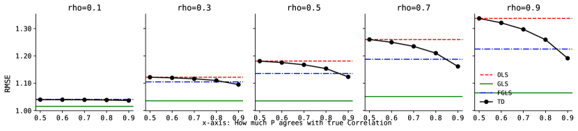
(a) bikeshare dataset

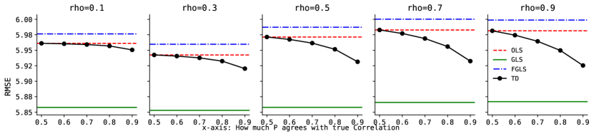
(b) house price dataset

Figure 5: Test Root Mean Squared Error (RMSE) versus different values of $P$ on bikeshare and execution time dataset. From left to right, the noise correlation coefficient increases ($\rho\in\{0.1,0.3,0.5,0.7,0.9\}$). Each plot’s x-axis represents the degree of alignment between the transition matrix $P$ and the true covariance matrix that generates the noise. Consistent with our expectations, as $P$ approaches the true correlation – implying a higher likelihood of data points with positively correlated noise transitioning from one to another – the solution derived from TD increasingly approximates the optimal one. Furthermore, as the correlation among the data intensifies, TD’s solution is closer to optimum and one can see larger gap between TD and OLS/FGLS. The results are averaged over $30$ runs.

C.3 Additional Results: Regression with Correlated Noise with NNs

Similar to that has been shown in  Figure 3, we show learning curves on increasingly strong correlated noise in  Figure 6. In this set of experiments, to speed up noise sampling, we randomly take $1$k subset of the original datasets for training and testing. The covariance matrix used to generate correlated noise is specified in Appendix B.

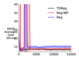
(a) House, $\sigma=10$

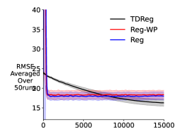
(b) House, $\sigma=20$

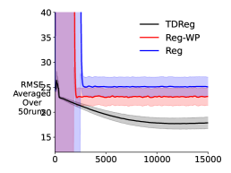
(c) House, $\sigma=30$

Figure 6: Learning curves on house dataset. From left to right, the noise variance increases, with $\sigma\in{10,20,30}$. The results are averaged over 50 runs. Due to the addition of large-scale noise, the two baseline algorithms, Reg-WP and Reg, exhibit high instability during the early learning stages and ultimately converge to a suboptimal solution compared to our TD approach.

C.4 Additional Results: Binary Classification with NNs

For binary classification, we utilize datasets from Australian weather (Joe Young, Owner), and travel insurance (Company, 2021). The aim of this series of experiments is to examine: 1) the impact of utilizing a link function; 2) with a specially designed transition probability matrix, the potential unique benefits of the TD algorithm in an imbalanced classification setting. Our findings indicate that: 1) the link function significantly influences performance; and 2) while the transition matrix proves beneficial in addressing class imbalance, this advantage seems to stem primarily from up/down-sampling rather than from the TD bootstrap targets.

Recall that we employ three intuitive types of transition matrices: $P(\mathbf{\bm{x}}^{\prime}|\mathbf{\bm{x}})$ is larger when the two points $\mathbf{\bm{x}},\mathbf{\bm{x}}^{\prime}$ are 1) similar (denoted as $P_{s}$); 2) far apart ($P_{f}$); 3) $P(\mathbf{\bm{x}}^{\prime}|\mathbf{\bm{x}})=1/n,\forall\mathbf{\bm{x}},\mathbf{\bm{x}}^{\prime}\in\mathcal{X}$ ($P_{c}$).

Since our results in Table 2 and Figure 4 indicate that $\mathbf{P}$ does not significantly impact regular regression, we conducted experiments on binary classification tasks and observed their particular utility when dealing with imbalanced labels. We define $P_{s}$ by defining the probability of transitioning to the same class as $0.9$ and to the other class as $0.1$. Table 5 presents the reweighted balanced results for three binary classification datasets with class imbalance. It is worth noting that in such cases, Classify-WP serves as both 1) no bootstrap baseline and 2) the upsampling techniques for addressing class imbalance in the literature (Kubát & Matwin, 1997).

Observing that TD-Classify and Classify-WP yield nearly identical results and Classify (without using TD’s sampling) is significantly worse, suggesting that the benefit of TD arises from the sampling distribution rather than the bootstrap estimate in the imbalanced case. Furthermore, $P_{f},P_{s}$ yield almost the same results in this scenario since they provide the same stationary distribution (equal weight to each class), so here Classify-WP represents both. We also conducted tests using $P_{c}$, which yielded results that are almost the same as Classify, and have been omitted from the table. In conclusion, the performance difference of TD in the imbalanced case arises from the transition probability matrix rather than the bootstrap target. The transition matrix’s impact is due to the implied difference in the stationary distribution.

	TD-Classify	Classify-WP	Classify	TD-WOF
Insurance	$0.0073\pm 0.0001$	$0.0073\pm 0.0001$	$0.0144\pm 0.0003$	$0.4994\pm 0.0005$
Weather	$0.0695\pm 0.0008$	$0.0701\pm 0.0008$	$0.0913\pm 0.0010$	$0.4965\pm 0.0031$

Table 5: Binary classification with imbalance. $0.0073$ means $0.73\%$ misclassification rate. The results are smoothed over $5$ evaluations before averaging over $5$ random seeds.

The usage of inverse link function. The results of TD on classification without using a transformation/link function are presented in Table 5 and are marked by the suffix ’WOF.’ These results are not surprising, as the bootstrap estimate can potentially disrupt the TD target entirely. Consider a simple example where a training example $\mathbf{\bm{x}}$ has a label of one and transitions to another example, also labeled one. Then the reward ($r=y-\gamma y^{\prime}$) will be $1-\gamma$. If the bootstrap estimate is negative, the TD target might become close to zero or even negative, contradicting the original training label of one significantly.

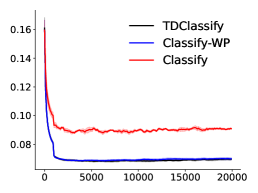
(a) weather

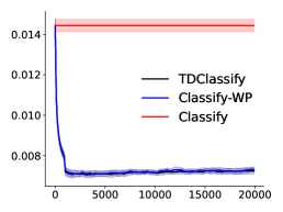
(b) insurance

Figure 7: Learning curves of binary classification with imbalance: balanced testing error v.s. training steps. The results have been smoothed using a $5$-point window before averaging over $5$ runs.

On binary classification dataset, weather and insurance, the imbalance ratios (proportion of zeros) are around $72.45\%,88.86\%$ respectively. We set number of iterations to $20$k for both and it is sufficient to see convergence. Additionally, in our TD algorithm, to prevent issues with inverse link functions, we add or subtract $1\times 10^{-15}$ when applying them to values of $0$ or $1$ in classification tasks. It should be noted that this parameter can result in invalid values depending on concrete loss implementation, usually setting $<10^{-7}$ should be generally good.

On those class-imbalanced datasets, when computing the reweighted testing error, we use the function from https://scikit-learn.org/stable/modules/generated/sklearn.metrics.balanced_accuracy_score.html.

C.5 On the Implementation of P

As we mentioned in Section 6, to investigate the effect of transition matrix, we implemented three types of transition matrices: $\mathbf{P}(\mathbf{\bm{x}}^{\prime}|\mathbf{\bm{x}})$ is larger when the two points $x,x^{\prime}$ 1) are similar; 2) when they are far apart; 3) $\mathbf{P}(\mathbf{\bm{x}}^{\prime}|\mathbf{\bm{x}})=1/n,\forall\mathbf{\bm{x}},\mathbf{\bm{x}}^{\prime}\in\mathcal{X}$. To expedite computations, $P_{s},P_{f}$ are computed based on the training targets instead of the features. The rationale for choosing these options is as follows: the first two may lead to a reduction in the variance of the bootstrap estimate if two consecutive points are positively or negatively correlated.

The resulting matrix may not be a valid stochastic matrix, we use DSM projection (Wang et al., 2010) to turn it into a valid one.

We now describe the implementation details. For first choice, given two points $(\mathbf{\bm{x}}_{1},y_{1}),(\mathbf{\bm{x}}_{2},y_{2})$, the formulae to calculate the similarity is:

$$k(y_{1},y_{2})=\exp(-(y_{1}-y_{2})^{2}/v)+0.1$$ (73)

where $v$ is the variance of all training targets divided by training set size. The second choice is simply $1-\exp(-(y_{1}-y_{2})^{2}/v)$.

Note that the constructed matrix may not be a valid probability transition matrix. To turn it into a valid stochastic matrix, we want: $\mathbf{P}$ itself must be row-normalized (i.e., $\mathbf{P}\mathbf{\bm{1}}=\mathbf{\bm{1}}$). To ensure fair comparison, we want equiprobable visitations for all nodes/points, that is, the stationary distribution is assumed to be uniform: $\mathbf{\bm{\pi}}=\frac{1}{n}\mathbf{\bm{1}}$.

The following proposition shows the necessary and sufficient conditions of the uniform stationary distribution property:

Proposition C.1.

$\mathbf{\bm{\pi}}=\frac{1}{n}\mathbf{\bm{1}}$ is the stationary distribution of an ergodic $\mathbf{P}$ if and only if $\mathbf{P}$ is a doubly stochastic matrix (DSM).

Proof.

If: Note that

$$\pi_{j}=\sum_{i}\pi_{i}p_{ij}\quad\text{and}\quad 1=\sum_{i}p_{ij}$$ (74)

Subtracting these two gives

$$1-\pi_{j}=\sum_{i}(1-\pi_{i})p_{ij}\quad\text{and}\quad\frac{1-\pi_{j}}{n}=\sum_{i}\frac{1-\pi_{i}}{n}p_{ij}.$$

This last equation indicates that $\left(\frac{1-\pi_{1}}{n},\frac{1-\pi_{2}}{n},\cdots,\frac{1-\pi_{n}}{n}\right)^{\top}$ is also the stationary distribution of $\mathbf{P}$. Due to the uniqueness of the stationary distribution, we must have

$$\frac{1-\pi_{i}}{n}=\pi_{i}$$

and thus $\pi_{i}=\frac{1}{n},\forall i$.

Only if: Since $\mathbf{\bm{\pi}}=\frac{1}{n}\mathbf{\bm{1}}$ is the stationary distribution of $\mathbf{P}$, we have

$$\frac{1}{n}\mathbf{\bm{1}}^{\top}\mathbf{P}=\frac{1}{n}\mathbf{\bm{1}}^{\top}$$

and thus $\mathbf{\bm{1}}^{\top}\mathbf{P}=\mathbf{\bm{1}}^{\top}$ showing that $\mathbf{P}$ is also column-normalized. ∎

With linear function approximation,

$$\mathbf{A} =\mathbf{X}^{\top}\mathbf{D}(\mathbf{I}-\gamma\lambda\mathbf{P})^{-1}(\mathbf{I}-\gamma\mathbf{P})\mathbf{X}$$ (75)

$$\mathbf{\bm{b}} =\mathbf{X}^{\top}\mathbf{D}(\mathbf{I}-\gamma\lambda\mathbf{P})^{-1}(\mathbf{I}-\gamma\mathbf{P})\mathbf{\bm{y}}$$ (76)

$$\mathbf{A} =\mathbf{X}^{\top}\mathbf{D}(\mathbf{I}-\gamma\mathbf{P})\mathbf{X}$$ (77)

$$\mathbf{\bm{b}} =\mathbf{X}^{\top}\mathbf{D}(\mathbf{I}-\gamma\mathbf{P})\mathbf{\bm{y}}$$ (78)

where $\mathbf{X}\in\mathbb{R}^{n\times d}$ is the feature matrix, and $\mathbf{D}$ is uniform when $\mathbf{P}$ is a DSM.

As a result, we can apply a DSM (Wang et al., 2010) projection method to our similarity matrix.

References

- Abadi et al. (2015) Abadi, M., Agarwal, A., Barham, P., and et al. TensorFlow: Large-scale machine learning on heterogeneous systems, 2015. Software available from tensorflow.org.
- Aitken (1936) Aitken, A. C. Iv.—on least squares and linear combination of observations. Proceedings of the Royal Society of Edinburgh, pp. 42–48, 1936.
- Baltagi (2008) Baltagi, B. H. Econometrics. Springer Books. Springer, 2008.
- Banerjee et al. (2005) Banerjee, A., Merugu, S., Dhillon, I. S., Ghosh, J., and Lafferty, J. Clustering with bregman divergences. Journal of machine learning research, 6(10), 2005.
- Bhandari et al. (2018) Bhandari, J., Russo, D., and Singal, R. A finite time analysis of temporal difference learning with linear function approximation. In Conference on learning theory, pp. 1691–1692. PMLR, 2018.
- Bishop (2006) Bishop, C. M. Pattern Recognition and Machine Learning. Springer, 2006.
- Bradtke & Barto (1996) Bradtke, S. J. and Barto, A. G. Linear least-squares algorithms for temporal difference learning. Machine Learning, 1996.
- Company (2021) Company, T. Travel insurance data, 2021. URL https://www.kaggle.com/datasets/tejashvi14/travel-insurance-prediction-data/data.
- Fanaee-T & Gama (2013) Fanaee-T, H. and Gama, J. Event labeling combining ensemble detectors and background knowledge. Progress in Artificial Intelligence, pp. 1–15, 2013.
- Ghosh et al. (2021) Ghosh, D., Gupta, A., Reddy, A., Fu, J., Devin, C. M., Eysenbach, B., and Levine, S. Learning to reach goals via iterated supervised learning. In International Conference on Learning Representations, 2021.
- Ghugare et al. (2024) Ghugare, R., Geist, M., Berseth, G., and Eysenbach, B. Closing the gap between td learning and supervised learning - a generalisation point of view. International Conference on Learning Representations, 2024.
- Greville (1966) Greville, T. N. E. Note on the generalized inverse of a matrix product. Siam Review, 8(4):518–521, 1966.
- Gupta et al. (2021) Gupta, D., Mihucz, G., Schlegel, M., Kostas, J., Thomas, P. S., and White, M. Structural credit assignment in neural networks using reinforcement learning. In Advances in Neural Information Processing Systems, pp. 30257–30270, 2021.
- He et al. (2016) He, K., Zhang, X., Ren, S., and Sun, J. Deep residual learning for image recognition. Computer Vision and Pattern Recognition (CVPR), pp. 770–778, 2016.
- Helmbold et al. (1999) Helmbold, D. P., Kivinen, J., and Warmuth, M. K. Relative loss bounds for single neurons. IEEE Transactions on Neural Networks, 10(6):1291–1304, 1999.
- Hussein et al. (2017) Hussein, A., Gaber, M. M., Elyan, E., and Jayne, C. Imitation learning: A survey of learning methods. ACM Comput. Surv., 2017.
- Joe Young (Owner) Joe Young (Owner), A. E. Rain in Australia, Copyright Commonwealth of Australia 2010, Bureau of Meteorology. https://www.kaggle.com/datasets/jsphyg/weather-dataset-rattle-package, 2020. URL http://www.bom.gov.au/climate/dwo/,http://www.bom.gov.au/climate/data.
- Kariya & Kurata (2004) Kariya, T. and Kurata, H. Generalized least squares. John Wiley & Sons, 2004.
- Kingma & Ba (2015) Kingma, D. P. and Ba, J. Adam: A method for stochastic optimization. International Conference on Learning Representations, 2015.
- Krizhevsky (2009) Krizhevsky, A. Learning multiple layers of features from tiny images. Technical report, 2009.
- Kubát & Matwin (1997) Kubát, M. and Matwin, S. Addressing the curse of imbalanced training sets: One-sided selection. International Conference on Machine Learning, 1997.
- LeCun et al. (2010) LeCun, Y., Cortes, C., and Burges, C. Mnist handwritten digit database. ATT Labs [Online]. Available: http://yann.lecun.com/exdb/mnist, 2, 2010.
- Lee et al. (2020) Lee, L., Eysenbach, B., Salakhutdinov, R., Gu, S. S., and Finn, C. Weakly-supervised reinforcement learning for controllable behavior. In Advances in Neural Information Processing Systems, 2020.
- Lichman (2015) Lichman, M. UCI machine learning repository, 2015. URL http://archive.ics.uci.edu/ml.
- Lin et al. (2020) Lin, E., Chen, Q., and Qi, X. Deep reinforcement learning for imbalanced classification. Applied Intelligence, pp. 2488–2502, 2020.
- MacGlashan et al. (2017) MacGlashan, J., Ho, M. K., Loftin, R., Peng, B., Wang, G., Roberts, D. L., Taylor, M. E., and Littman, M. L. Interactive learning from policy-dependent human feedback. In International Conference on Machine Learning, pp. 2285–2294, 2017.
- Maei (2011) Maei, H. R. Gradient temporal-difference learning algorithms. 2011.
- McCullagh & Nelder (1989) McCullagh, P. and Nelder, J. A. Generalized Linear Models, volume 37. CRC Press, 1989.
- Mnih et al. (2015) Mnih, V., Kavukcuoglu, K., Silver, D., Rusu, A. A., and et al. Human-level control through deep reinforcement learning. Nature, 2015.
- Nelder (1974) Nelder, J. A. Log linear models for contingency tables: A generalization of classical least squares. Journal of the Royal Statistical Society. Series C (Applied Statistics), pp. 323–329, 1974.
- Nelder & Wedderburn (1972) Nelder, J. A. and Wedderburn, R. W. M. Generalized linear models. Journal of the Royal Statistical Society. Series A (General), pp. 370–384, 1972.
- Pan et al. (2017a) Pan, Y., Azer, E. S., and White, M. Effective sketching methods for value function approximation. Conference on Uncertainty in Artificial Intelligence, 2017a.
- Pan et al. (2017b) Pan, Y., White, A., and White, M. Accelerated gradient temporal difference learning. AAAI Conference on Artificial Intelligence, pp. 2464–2470, 2017b.
- Pan et al. (2020) Pan, Y., Imani, E., Farahmand, A.-m., and White, M. An implicit function learning approach for parametric modal regression. Advances in Neural Information Processing Systems, 33:11442–11452, 2020.
- Paredes & Ballester-Ripoll (2018) Paredes, E. and Ballester-Ripoll, R. SGEMM GPU kernel performance. UCI Machine Learning Repository, 2018.
- Paszke et al. (2017) Paszke, A., Gross, S., Chintala, S., Chanan, G., Yang, E., DeVito, Z., Lin, Z., Desmaison, A., Antiga, L., and Lerer, A. Automatic differentiation in pytorch. 2017.
- Perdomo et al. (2020) Perdomo, J., Zrnic, T., Mendler-Dünner, C., and Hardt, M. Performative prediction. International Conference on Machine Learning, pp. 7599–7609, 2020.
- Puterman (2014) Puterman, M. L. Markov decision processes: discrete stochastic dynamic programming. John Wiley & Sons, 2014.
- Seabold & Perktold (2010) Seabold, S. and Perktold, J. statsmodels: Econometric and statistical modeling with python. In 9th Python in Science Conference, 2010.
- Sutton (1988) Sutton, R. S. Learning to predict by the methods of temporal differences. Machine Learning, pp. 9–44, 1988.
- Sutton et al. (2016) Sutton, R. S., Mahmood, A. R., and White, M. An emphatic approach to the problem of off-policy temporal-difference learning. Journal of Machine Learning Research, 2016.
- Szepesvari (2010) Szepesvari, C. Algorithms for Reinforcement Learning. Morgan & Claypool Publishers, 2010.
- Tsitsiklis & Van Roy (1997) Tsitsiklis, J. N. and Van Roy, B. An analysis of temporal-difference learning with function approximation. IEEE Transactions on Automatic Control, 42(5), 1997.
- Wang et al. (2010) Wang, F., Li, P., and Konig, A. C. Learning a bi-stochastic data similarity matrix. In 2010 IEEE International Conference on Data Mining, pp. 551–560. IEEE, 2010.
- Xiao et al. (2022) Xiao, C., Dai, B., Mei, J., Ramirez, O. A., Gummadi, R., Harris, C., and Schuurmans, D. Understanding and leveraging overparameterization in recursive value estimation. In International Conference on Learning Representations, 2022.
- Xiao et al. (2017) Xiao, H., Rasul, K., and Vollgraf, R. Fashion-mnist: a novel image dataset for benchmarking machine learning algorithms. CoRR, 2017. URL http://arxiv.org/abs/1708.07747.