A Rotational/Roto-translational Constraint Method for Condensed Matter

Abstract

In condensed matter physics, particularly in perovskite materials, the rotational motion of molecules and ions is associated with important issues such as ion conduction mechanism. Constrained Molecular Dynamics (MD) simulations offer a means to separate translational, vibrational, and rotational motions, enabling the independent study of their effects. In this study, we introduce a rotational and roto-translational constraint algorithm based on the Velocity Verlet integrator, which has been implemented into a homebrew version of the CP2K package. The MD results show that our program can selectively constrain the molecules and ions in the system and support long-time MD runs. The algorithm can help the future study of important rotation-related dynamic problems in condensed matter systems.

jlu] Institute of Theoretical Chemistry, College of Chemistry, Jilin University, 2519 Jiefang Road, Changchun 130023, P.R.China jlu] Institute of Theoretical Chemistry, College of Chemistry, Jilin University, 2519 Jiefang Road, Changchun 130023, P.R.China jlu] Institute of Theoretical Chemistry, College of Chemistry, Jilin University, 2519 Jiefang Road, Changchun 130023, P.R.China jlu] Institute of Theoretical Chemistry, College of Chemistry, Jilin University, 2519 Jiefang Road, Changchun 130023, P.R.China IR,NMR,UV

1 Introduction

Rotation of molecules/ions in condensed matter, especially in perovskite crystals, can have close relation with important problems: the molecular rotation can drive phase transition in amorphous ice¹; the volumetric lattice strain and CH3NH3 molecular rotational degrees of freedom(DOF) can cooperate to create and stabilize polarons in perovskite solar cell materials²; in the study of solid electrolytes, anion rotation is associated with fast ion conduction, the coupling between anion rotation and cation diffusion is named as paddle-wheel mechanism which has drawn general interest³.

Experimental techniques can provide statistically averaged information on molecule/ion rotation. When combined with ab initio molecular dynamics(AIMD), further microscopic information can be obtained. In addition, fixing the motion of molecules/ions in AIMD allows for an approximate calculation of the rotation effect on material properties^{4, 5, 6}. However, in these studies, vibration and translation of the molecules/ions were also fixed. A more rational approach would be to fix only the rotation of the molecules/ions.

The Nola group derived a roto-translational constraint algorithm ⁷. Their method has been implemented in GROMOS⁸ and GROMACS⁹. They hope that the algorithm will improve the efficiency of molecular dynamics(MD) running and be used in molecular docking research. Their work is rigorous and original, however, the method is implemented from a biomolecule perspective and based on the leap frog integrator¹⁰. Most popular material MD software, including LAMMPS¹¹, VASP^{12, 13}, and CP2K¹⁴, do not support the leap frog integrator, which hindered the application of the method to condensed matter.

The application of rotational constraint in AIMD is also a problem. Most biomolecule simulation software is specialized in MD simulations using the empirical force field or simple QM/MM methods^{15, 16}, and do not support AIMD. The interfaces of biomolecule simulation software are improving, for instance, GROMACS can be combined with CP2K to use the quantum mechanical/molecular mechanical(QM/MM) method. However, it is still not as convenient and efficient as implementing the constraint algorithms directly in material simulation software. To apply the rotational constraint algorithm in AIMD, it is necessary to rely on software such as VASP, CP2K, etc.

The Krimm group derived a general constraint algorithm named WIGGLE¹⁷; an angular momentum constraint method was mentioned in their work. The constrained accelerations are used in their derivation. They claimed that the WIGGLE algorithm is almost an order of magnitude more accurate than the RATTLE algorithm, but the algorithm is rarely used, probably because it has not been implemented in popular dynamics software.

To the best of our knowledge, there is no popular material simulation software that implements the rotational constraint algorithm. This work presents a rotational/roto-translational constraint algorithm based on the Velocity Verlet integrator¹⁸, which is commonly used in materials simulation software. The algorithm has been implemented into a homebrew version of the CP2K program, and has been tested in MD running. The results indicate that our program can selectively constrain the rotational/roto-translational motions of molecules in the system and support stable long-time runs.

2 Theory

The theoretical derivation of the rotational constraints using the Velocity Verlet integrator is presented in this section. Our derivation follows the RATTLE algorithm¹⁹, which is widely applied in MD software. Constraints for linear molecules are special cases and are not discussed in this work. Since the roto-translational constraints differ only in the initial conditions from the rotational constraints, their derivation is presented in the supporting information.

We describe the constrained atoms using the center-of-mass(COM) coordinates system for convenience:

$$\mathbf{r}_{a}=\mathbf{R}_{a}-\frac{\sum_{a=1}^{n_{a}}m_{a}\mathbf{R}_{a}}{\sum_{a=1}^{n_{a}}m_{a}},$$ (1)

$$\sum_{a=1}^{n_{a}}m_{a}\mathbf{r}_{a}=\mathbf{0}.$$

$n_{a}$ is the total number of constrained atoms, $m_{a}$ is the mass of $a$th atom. $\mathbf{R}_{a}$ is the position vector of $a$th atom in Cartesian coordinates system, while $\mathbf{r}_{a}$ is the position vector of $a$th atom in the COM coordinates system.

We use the same rotational constraint conditions as Amadei groups⁷.

$$\boldsymbol{\chi}^{(r)}=\sum^{n_{a}}_{a=1}\mathbf{r}^{0}_{a}\times m_{a}\mathbf{r}_{a}(t)=\mathbf{0}.$$ (2)

The superscript $r$ indicates the quantity corresponds to a positional constraint, and $\mathbf{r}_{a}^{0}$ is the rotational reference position of $a$th atom. Another option is to use condition equations without mass. We prefer the condition equations with mass because it is close to the rotational Eckart conditions which divide the nuclear motion into translations, rotations, and vibrations approximately²⁰.

The constraints are applied to the whole molecule, some bond wiggling is allowed. In particular, if some atom’s rotational reference position is at the COM($\mathbf{r}_{a}^{0}=\mathbf{0}$), the atom will be constrained in a manner that is related to the COM and has no direct contribution to the constraint conditions.

Differentiating the equations at time $t$ yields the velocity constraints

$$\boldsymbol{\chi}^{(v)}=\sum^{n_{a}}_{a=1}\mathbf{r}^{0}_{a}\times m_{a}\mathbf{v}_{a}(t)=\mathbf{0}.$$ (3)

The superscript $v$ indicates the quantity corresponds to a velocity constraint, $\mathbf{v}_{a}(t)$ is the velocity of $a$th atom at time $t$. The rotational reference positions are constants. If we replace $\mathbf{r}_{a}^{0}$ with $\mathbf{r}_{a}(t)$, $\boldsymbol{\chi}^{(v)}$ will be the total angular moment of the constrained atoms.

Verlocity Verlet integrator has position part and velocity part

$$\mathbf{r}_{a}(t+\delta t)=\mathbf{r}_{a}(t)+\delta t\,\mathbf{v}_{a}(t)+\frac{1}{2m_{a}}\delta t^{2}\mathbf{f}_{a}(t),$$ (4)

$$\mathbf{v}_{a}(t+\delta t)=\mathbf{v}_{a}(t)+\frac{1}{2m_{a}}\delta t\left(\mathbf{f}_{a}(t)+\mathbf{f}_{a}(t+\delta t)\right).$$

Consider the position part with the constraint force first

$$\mathbf{r}_{a}(t+\delta t)=\mathbf{r}_{a}^{\prime}(t+\delta t)+\frac{1}{2m_{a}}\delta t^{2}\mathbf{g}_{a}^{(\mathrm{r})}(t).$$ (5)

$\mathbf{g}_{a}^{(\mathrm{r})}$ is the positional constraint force on $a$th atom, the prime symbol in $\mathbf{r}_{a}^{\prime}$ indicates the quantities without constraints. Multiply both sides of the equation by $m_{a}$, cross product both sides of the equation by $\mathbf{r}_{a}^{0}$ from left, then sum over atoms, we get

$$\sum^{n_{a}}_{a=1}\mathbf{r}_{a}^{0}\times m_{a}\mathbf{r}_{a}(t+\delta t)=\sum^{n_{a}}_{a=1}\mathbf{r}_{a}^{0}\times[m_{a}\mathbf{r}_{a}^{\prime}(t+\delta t)+\frac{1}{2}\delta t^{2}\,\mathbf{g}_{a}^{(\mathrm{r})}(t)].$$ (6)

The left side of the equation is the same as our rotational constraint conditions Eq. (2), which should be zero at anytime. So

$$\sum^{n_{a}}_{a=1}\mathbf{r}_{a}^{0}\times[m_{a}\mathbf{r}_{a}^{\prime}(t+\delta t)+\frac{1}{2}\delta t^{2}\,\mathbf{g}_{a}^{(\mathrm{r})}(t)]=\mathbf{0}.$$ (7)

The positional constraint force can be written as

$$\mathbf{g}_{a}^{(r)}=-\sum_{i=1}^{n_{r}}\lambda_{i}^{(r)}\nabla_{\!\mathbf{r}_{a}}\,\chi_{i}^{(r)}.$$ (8)

$n_{r}$ is the number of DOF are constrainted, $n_{r}=3$ in rotational constraint for nonlinear molecule. $\lambda_{i}^{(r)}$ is the $i$th Lagrange multipliers of position constraint. The minus symbol on the right side is just for definition because we can write it into the $\lambda_{i}^{(r)}$.

Substitute Eq. (2) into Eq. (8). Take $(x_{1},y_{1},z_{1},x_{2},y_{2},z_{2},\dots,x_{a},y_{a},z_{a})$ as atoms position in COM coordinate system, $(X_{1},Y_{1},Z_{1},X_{2},Y_{2},Z_{2},\dots,X_{a},Y_{a},Z_{a})$ as atoms position of rotational reference in COM coordinate system. We get

$$g_{a,x}^{(r)}=-\sum_{i=1}^{n_{r}}\lambda_{i}^{(r)}\frac{\partial\chi_{i}^{(r)}}{\partial x_{a}}=m_{a}\left(-Z_{a}\lambda_{2}^{(r)}+Y_{a}\lambda_{3}^{(r)}\right),$$ (9)

$$g_{a,y}^{(r)}=-\sum_{i=1}^{n_{r}}\lambda_{i}^{(r)}\frac{\partial\chi_{i}^{(r)}}{\partial y_{a}}=m_{a}\left(\ \ Z_{a}\lambda_{1}^{(r)}-X_{a}\lambda_{3}^{(r)}\right),$$

$$g_{a,z}^{(r)}=-\sum_{i=1}^{n_{r}}\lambda_{i}^{(r)}\frac{\partial\chi_{i}^{(r)}}{\partial z_{a}}=m_{a}\left(-Y_{a}\lambda_{1}^{(r)}+X_{a}\lambda_{2}^{(r)}\right).$$

Define

$$\mathbf{c}^{(r)}=\sum_{a=1}^{n_{a}}\mathbf{r}_{a}^{0}\times m_{a}\mathbf{r}_{a}^{\prime}(t+\delta t).$$ (10)

Substitute Eq. (9) and Eq. (10) into Eq. (7), we will get equations

$$\begin{cases}\mathbf{c}_{x}^{(r)}+\sum\limits_{a=1}^{n_{a}}\frac{1}{2}m_{a}\delta t^{2}\left(-\left(Y_{a}^{2}+Z_{a}^{2}\right)\lambda_{1}^{(r)}+X_{a}Y_{a}\lambda_{2}^{(r)}+X_{a}Z_{a}\lambda_{3}^{(r)}\right)=0\\ \mathbf{c}_{y}^{(r)}+\sum\limits_{a=1}^{n_{a}}\frac{1}{2}m_{a}\delta t^{2}\left(\ \ \ X_{a}Y_{a}\lambda_{1}^{(r)}-\left(X_{a}^{2}+Z_{a}^{2}\right)\lambda_{2}^{(r)}+Y_{a}Z_{a}\lambda_{3}^{(r)}\right)=0\\ \mathbf{c}_{z}^{(r)}+\sum\limits_{a=1}^{n_{a}}\frac{1}{2}m_{a}\delta t^{2}\left(\ \ \,X_{a}Z_{a}\lambda_{1}^{(r)}+Y_{a}Z_{a}\lambda_{2}^{(r)}-\left(X_{a}^{2}+Y_{a}^{2}\right)\lambda_{3}^{(r)}\right)=0.\end{cases}$$ (11)

In matrix form is

$$\mathbf{c}^{(r)}+\boldsymbol{\Theta}^{(r)}\boldsymbol{\lambda}^{(r)}=\mathbf{0},$$ (12)

$$\boldsymbol{\lambda}^{(r)}=-\left(\boldsymbol{\Theta}^{(r)}\right)^{-1}\mathbf{c}^{(r)}.$$

Then we can solve all Lagrange multipliers $\boldsymbol{\lambda}^{(r)}$. From Eq. (9) and Eq. (5) we can get constraint force and constrained positions at the next time step $\mathbf{r}_{a}(t+\delta t)$.

The velocity part of Velocity Verlet integrator with constraint force is

$$\mathbf{v}_{a}(t+\delta t)=\mathbf{v}_{a}^{\prime}(t+\delta t)+\frac{1}{2m_{a}}\delta t\,\mathbf{g}_{a}^{(\mathrm{v})}(t+\delta t).$$ (13)

$\mathbf{g}_{a}^{(\mathrm{v})}$ is the velocity constraint force on $a$th atom. As we have done in the position part, we multiply both sides of the equation by $m_{a}$, cross product both sides of the equation by $\mathbf{r}_{a}^{0}$ from left, then sum over atoms

$$\sum_{a=1}^{n_{a}}\mathbf{r}_{a}^{0}\times m_{a}\mathbf{v}_{a}(t+\delta t)=\sum_{a=1}^{n_{a}}\mathbf{r}_{a}^{0}\times\left[m_{a}\mathbf{v}_{a}^{\prime}(t+\delta t)+\frac{1}{2}\delta t\,\mathbf{g}_{a}^{(\mathrm{v})}(t+\delta t)\right].$$ (14)

From Eq. (3)

$$\sum_{a=1}^{n_{a}}\mathbf{r}_{a}^{0}\times[m_{a}\mathbf{v}_{a}^{\prime}(t+\delta t)+\frac{1}{2}\delta t\,\mathbf{g}_{a}^{(\mathrm{v})}(t+\delta t)]=\mathbf{0}.$$ (15)

Eq. (3) is a semi-holonomic constraint condition. The corresponding constraint force is²¹

$$\mathbf{g}_{a}^{(v)}=-\sum^{n_{v}}_{i=1}\lambda_{i}^{(v)}\boldsymbol{\nabla}_{\!\mathbf{v}_{a}}\,\chi_{i}^{(v)}$$ (16)

Note that the gradient is with respect to the velocity $\mathbf{v}_{a}$ rather than positions. The rotational reference positions are constants, so the components of $\mathbf{g}_{a}^{(\mathrm{v})}$ has the same formalism as $\mathbf{g}_{a}^{(\mathrm{r})}$ in Eq. (9)

$$g_{a,x}^{(v)}=-\sum_{i=1}^{n_{v}}\lambda_{i}^{(v)}\frac{\partial\chi_{i}^{(v)}}{\partial v_{a,x}}=m_{a}\left(-Z_{a}\lambda_{2}^{(v)}+Y_{a}\lambda_{3}^{(v)}\right),$$ (17)

$$g_{a,y}^{(v)}=-\sum_{i=1}^{n_{v}}\lambda_{i}^{(v)}\frac{\partial\chi_{i}^{(v)}}{\partial v_{a,y}}=m_{a}\left(\;\;Z_{a}\lambda_{1}^{(v)}-X_{a}\lambda_{3}^{(v)}\right),$$

$$g_{a,z}^{(v)}=-\sum_{i=1}^{n_{v}}\lambda_{i}^{(v)}\frac{\partial\chi_{i}^{(v)}}{\partial v_{a,z}}=m_{a}\left(-Y_{a}\lambda_{1}^{(v)}+X_{a}\lambda_{2}^{(v)}\right).$$

Define

$$\mathbf{c}^{(v)}=\sum_{a=1}^{n_{a}}\mathbf{r}_{a}^{0}\times m_{a}\mathbf{v}_{a}^{\prime}(t+\delta t).$$ (18)

Substitute Eq. (17) and Eq. (18) into Eq. (15) we will get

$$\begin{cases}\mathbf{c}_{x}^{(v)}+\sum\limits_{a=1}^{n_{a}}\frac{1}{2}m_{a}\delta t\left(-\left(Y_{a}^{2}+Z_{a}^{2}\right)\lambda_{1}^{(v)}+X_{a}Y_{a}\lambda_{2}^{(v)}+X_{a}Z_{a}\lambda_{3}^{(v)}\right)=0\\ \mathbf{c}_{y}^{(v)}+\sum\limits_{a=1}^{n_{a}}\frac{1}{2}m_{a}\delta t\left(\quad X_{a}Y_{a}\lambda_{1}^{(v)}-\left(X_{a}^{2}+Z_{a}^{2}\right)\lambda_{2}^{(v)}+Y_{a}Z_{a}\lambda_{3}^{(v)}\right)=0\\ \mathbf{c}_{z}^{(v)}+\sum\limits_{a=1}^{n_{a}}\frac{1}{2}m_{a}\delta t\left(\quad\!X_{a}Z_{a}\lambda_{1}^{(v)}+Y_{a}Z_{a}\lambda_{2}^{(v)}-\left(X_{a}^{2}+Y_{a}^{2}\right)\lambda_{3}^{(v)}\right)=0.\end{cases}$$ (19)

In matrix form is

$$\mathbf{c}^{(v)}+\boldsymbol{\Theta}^{(v)}\boldsymbol{\lambda}^{(v)}=\mathbf{0},$$ (20)

$$\boldsymbol{\lambda}^{(v)}=-\left(\boldsymbol{\Theta}^{(v)}\right)^{-1}\mathbf{c}^{(v)}.$$

Then $\mathbf{\lambda}_{a}^{(v)},\,\mathbf{g}_{a}^{(v)}$ and the next step velocity $\mathbf{v}_{a}(t+\delta t)$ are solved.

Using inverse matrix method to solve the Lagrange multipliers is usually considered to be slow. However, no matter how many atoms are in one rotational constraint, the constrained DOF are only 3(6 for roto-translational constraint); we only need to ask for the inverse of two $3\times 3$($6\times 6$ for roto-translational constraint) matrices. Therefore, using inverse matrix method should be acceptable.

At the next step, we compute all the Lagrange multipliers, constrained positions, and constrained velocities again, then loop until the end of MD.

3 Program implementation and results

3.1 Program implementation

3.1.1 Basic usage

We implemented the program in a homebrew version of CP2K v8.2 package¹⁴. The basic usage of the program can be shown in a sample input file:

⬇

1…

2&COORD !Cartesian coordinates of system

3 N -0.00000000 0.00000000 -0.09999998 M1

4 H 0.00000000 0.95223715 0.23666663 M1

5 H 0.82466156 -0.47611858 0.23666663 M1

6 H -0.82466156 -0.47611858 0.23666663 M1

7 N 1.61846237 3.12648673 1.12207349 M2

8 H 1.61846237 4.07872389 1.45874010 M2

9 H 2.44312393 2.65036816 1.45874010 M2

10 H 0.79380080 2.65036816 1.45874010 M2

11 N -0.94386640 -1.51381415 2.30701324 M3

12 H -0.94386640 -0.56157700 2.64367985 M3

13 H -0.11920484 -1.98993273 2.64367985 M3

14 H -1.76852797 -1.98993273 2.64367985 M3

15&END

16…

17&CONSTRAINT !Constraint settings

18 CONSTRAINT_INIT T

19 &ROTC !Rotational/roto-translational constraint settings

20 MOLNAME M1

21 ATOMS 1 2 3 4

22 POSITIONS0 [ANGSTROM] -0.00000000 0.00000000 -0.09999998 0.00000000 0.95223715 0.23666663 0.82466156 -0.47611858 0.23666663 -0.82466156 -0.47611858 0.23666663

23 &END ROTC

24&END CONSTRAINT

In this file we fixed the rotation of one ammonia molecule which named as M1, and the other two ammonia molecules M2 and M3 are free of constraints. Only related text in the input file is shown. Different input blocks are divided by symbol &. Lines 2–15 are coordinates of the system. The first column is the elements of atoms, the followed three columns are the Cartesian coordinates in Angstrom. The last column is the molecule names which are defined as M1, M2, and M3 in the file. Lines 17–24 are settings for the constraints. Lines 19–23 correspond to the “ROTC” block which controls the rotational constraints. “MOLNAME M1” indicates the name which will be constrained is M1. “ATOMS 1 2 3 4” indicates atoms 1–4 in M1 will be constrained. “POSITIONS0 …” is the rotational reference coordinates at Cartesian coordinates in sequence $(x_{1},y_{1},z_{1},x_{2},y_{2},z_{2},x_{3},y_{3},z_{3},...)$, the unit is Angstrom. “POSITIONS0 …” will be transferred to the COM coordinates automatically in the program, which corresponds to the rotational reference coordinates $(X_{1},Y_{1},Z_{1},X_{2},Y_{2},Z_{2},\dots,X_{a},Y_{a},Z_{a})$ in the Eq.(9). The usage of roto-translational constraint algorithm is same as rotational constraint, the algorithm is implemented in another homebrew version of CP2K v8.2.

3.1.2 Center-of-mass definition with periodic boundary condition

Users should note that the definition of the rotational reference center is not unique when using periodic boundary conditions. As shown in Fig. 1, the box in the figure represents the simulation box with the periodic boundary, A and B denote two atoms close to the boundary of the box, and A^′ denotes the image of atom A due to periodicity. If the size of the molecule AB is comparable to the size of the box, as in Fig. 1(a), its center of mass, i.e., the rotational reference center, will be at a point O halfway between A and B. If the molecule AB is smaller than half the length of the box, as in Fig. 1(b), the rotational reference center will be at the point O^′ between A^′ and B. Even if we directly define the two atoms A and B as belonging to the same molecule in the input file, we still cannot avoid this ambiguity, so we use Cartesian coordinates to distinguish the two different cases. In CP2K, as long as “CENTER_COORDINATES” is set as False or default, the coordinates in the input file will be entered as they are, then we can deal with this question automatically by the program. If the molecule corresponds to the case in Fig. 1(a), the coordinates of atoms A and B can be defined directly, on the contrary, if the molecule corresponds to the case in Fig. 1(b), then the coordinates of A^′ and B should be defined, instead of the coordinates of A and B.

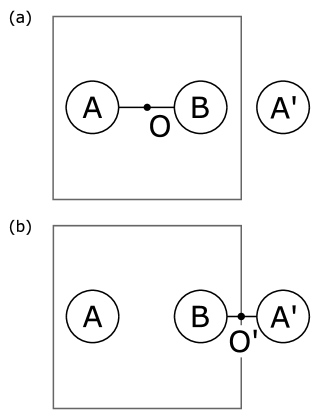
Figure 1: Two different rotational reference center definitions with periodic boundary condition.

3.1.3 Computational details

The running details of the MD trajectory results are as follows: The system consists of three ammonia molecules, as in Fig. 2. The HFX (Hartree-Fock exchange) basis set^{22, 23} and the GTH pseudopotentials²⁴ are used in the AIMD simulation. The simulation box is a cube of 10 Å side length, periodic boundary condition is used. In force field molecular dynamics(FFMD), Amber format force field²⁵ and 25 Å side length box is used for the modeling. The initial temperature is 300 K. The time step is 1 femtosecond, and the length of each trajectory is 2 picoseconds. The NVE and the NVT ensemble are used. The NOSÉ thermostator^{26, 27} is used in the NVT ensemble, and the temperature is set as 300 K. Only AIMD results are shown below. FFMD results are in the Supporting Information. All MD results ran with homebrew version codes of CP2K v8.2.

3.2 AIMD results

3.2.1 Rotational constraint results

The snapshot of NVE ensemble AIMD trajectory using rotational constraints are shown in Fig. 2(a)(t = 0 fs) and Fig. 2(b)(t = 320 fs). One can check animate graphs in the Supporting Information for more direct view. The result shows the molecule M3 moves normally, and the other two constrained molecules M1 and M2 do not rotate while vibrating and translating, which means our program meets the expectation. We define rotational constraint error as the norm of deviation from Eq. (2)

$$\sigma=\left\|\sum^{n_{a}}_{a=1}\mathbf{r}^{0}_{a}\times m_{a}\mathbf{r}_{a}(t)\right\|.$$ (21)

In AIMD the max error is $\sigma_{\max}=9.43\times 10^{-7}$ Å, and in FFMD the max error is $\sigma_{\max}=1.52\times 10^{-6}$ Å, which are close to numerical errors.

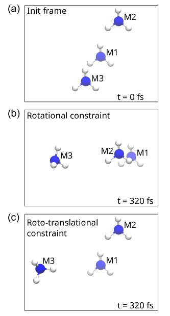
Figure 2: Snapshots of AIMD trajectory: (a) The init frame of AIMD; (b) The snapshot of trajectory using rotational constraint at 320 fs. Molecules M1 and M2 are constrained; (c) The snapshot of trajectory using roto-translational constraint at 320 fs. Molecules M1 and M2 are constrained. More intuitive animate graphs of trajectories are in Supporting Information.

One import question is the numerical stability of the program and insuring the errors will not accumulate during the running of MD. We statistic the fluctuations of conserved quantity, potential and temperature in trajectories, then compare the data with MD without constraints. The results of AIMD are shown in Fig. 3–4. More results of comparison of FFMD with/without constraints are in Supporting Information. The constant quantity(Cons. Qty.) indicates the number stability of the MD. It corresponds to the total energy in NVE ensemble, and in the NVT ensemble, it corresponds to the total energy of the system containing DOF of the heat bath. The difference of conserved quantity with/without constraints comes from the DOF change by constraints. The results show that no significant difference in the fluctuation size of conserved quantity, potential and temperature.

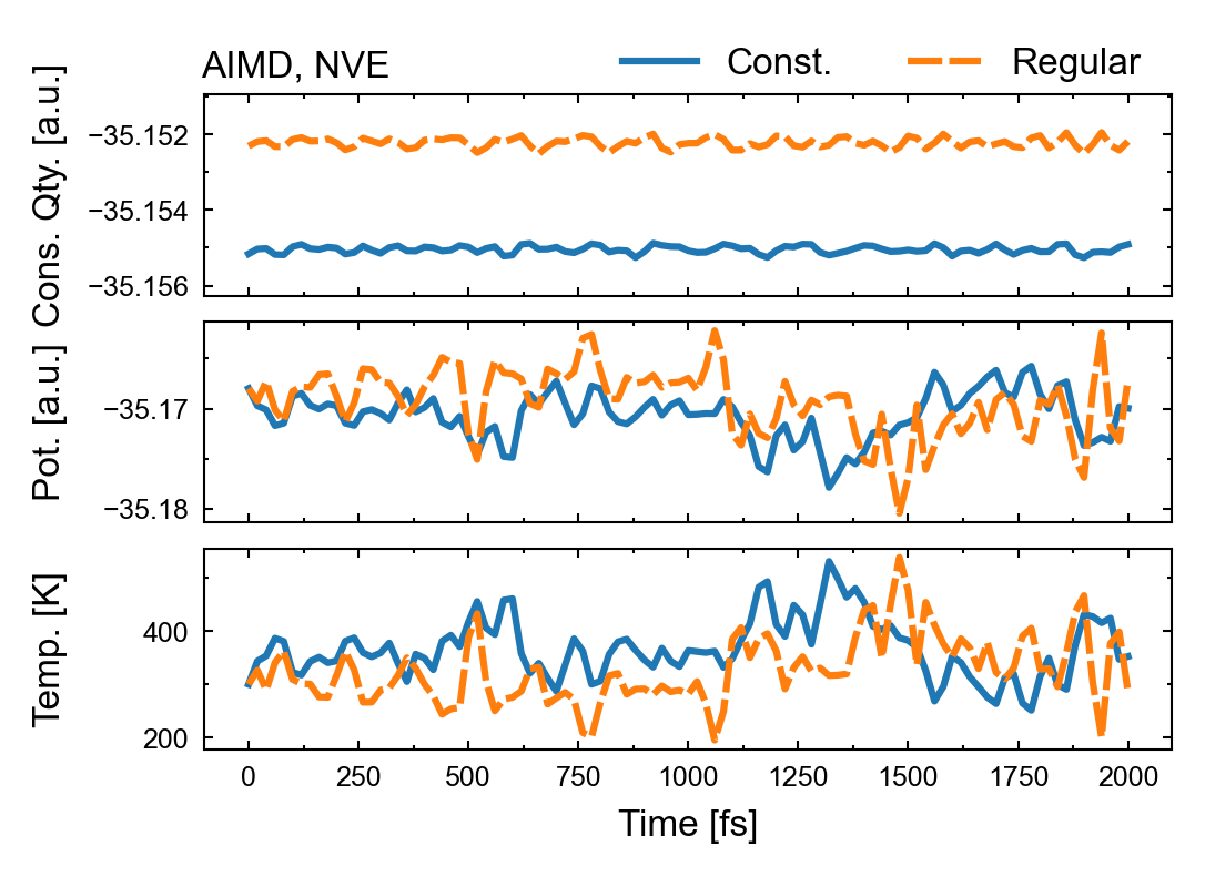
Figure 3: Conserved quantity(Cons. Qty.), potential(Pot.), and temperature(Temp.) fluctuation of the AIMD trajectory of NVE ensemble with/without rotational constraints(Const./Regular).

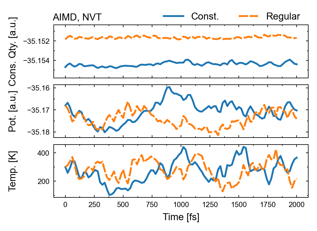
Figure 4: Conserved quantity(Cons. Qty.), potential(Pot.), and temperature(Temp.) fluctuation of the AIMD trajectory of NVT ensemble with/without rotational constraints(Const./Regular).

We also computed the drift and fluctuation of conserved quantity by least-squares fitting. We performed a least-squares fit of data to a straight line respectively. The drift is defined as the difference of the fit at the first and last point. The fluctuation is defined as the root mean square deviation(RMSD) around the least-squares fit. All drift/fluctuation difference from the no constraint MD is showed in Table 1. Most drift and fluctuation difference values are little than $1\times 10^{-4}$ a.u. The drift difference in AIMD using NVT ensemble showed a little bigger result with $2.57\times 10^{-4}$ a.u., which may caused by the collision of two ammonia molecules in the trajectory.

MD type	Ensemble		$\Delta_{\text{RC}}\,^{\text{a}}$	$\Delta_{\text{RTC}}\,^{\text{b}}$
Ab initio	NVE	Drift	$0.01$	$0.10$
		Fluc.	$0.36$	$0.26$
	NVT	Drift	$2.57$	$0.11$
		Fluc.	$0.58$	$0.50$
Force field	NVE	Drift	$0.03$	$0.02$
		Fluc.	$0.07$	$0.06$
	NVT	Drift	$0.13$	$0.07$
		Fluc.	$0.12$	$0.10$

• $\,{}^{\text{a}}$Rotational constraint

• $\,{}^{\text{b}}$Roto-translational constraint

• *The unit of data is $1\times 10^{-4}$ a.u.

Table 1: Drift and fluctuation(Fluc.) difference of conserved quantity between constrained MD and regular MD, which indicates the numerical stability.

3.2.2 Roto-translational constraint results

The snapshot of NVE ensemble AIMD trajectory using roto-translational constraints are shown in Fig. 2(a)(t = 0 fs) and Fig. 2(c)(t = 320 fs). One can check animate graphs in the Supporting Information for more direct view. The result shows the molecule M3 moves normally, and the other two constrained molecules M1 and M2 do not rotate or translate while vibrating, which means our program meets the expectation. We define the rotational constraint error same as in Eq. (21). In AIMD the max rotational error is $\sigma_{\max}=3.54\times 10^{-7}$ Å, and in FFMD the max rotational error is $\sigma_{\max}=4.83\times 10^{-6}$ Å. The translational error is defined as $\tau=\left\|\mathbf{C}^{0}-\mathbf{C}(t)\right\|$, which is the vector norm of change of center-of-mass $\mathbf{C}$. In AIMD the max translational error is $\tau_{\max}=1.00\times 10^{-6}$ Å, and in FFMD the max translational error is $\tau_{\max}=5.04\times 10^{-7}$ Å, , which are close to numerical error. The results of statistic fluctuation is similar with rotational constraint, which is showed in Fig. 5–6, no significant difference from the regular MD. The drift and fluctuation difference values are in Table 1. The results shows that the roto-translatonal constraint has a good numerical stability.

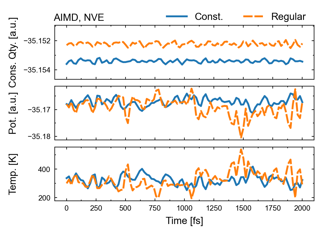
Figure 5: Conserved quantity(Cons. Qty.), potential(Pot.), and temperature(Temp.) fluctuation of the AIMD trajectory of NVE ensemble with/without roto-translational constraints(Const./Regular).

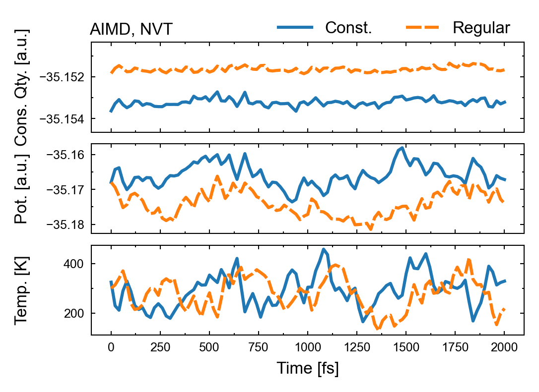
Figure 6: Conserved quantity(Cons. Qty.), potential(Pot.), and temperature(Temp.) fluctuation of the AIMD trajectory of NVT ensemble with/without roto-translational constraints(Const./Regular).

There is a small difference in initial temperature between constrained MD and regular MD. We set the initial temperature to 300 K in all MD results, when using the roto-translational constraint, the initial temperature is always a little higher than our settings, in Fig. 5–6 is about 336K. To explain this, we need to understand what is actually happening in the program. Typically, the constraint algorithm does nothing at the zeroth step of MD. After initializing the atomic velocity according to the set temperature, usually the atomic velocity of the system does not satisfy the constraint condition. Then we apply the constraint to the system, which will do work on the system and cause a change in the total energy. Once the constraint condition is satisfied at a certain step, the constraint algorithm will theoretically do no work on the system at subsequent steps in the MD. This will be shown as a leap in total energy only from zeroth to the first step.

In order to avoid the total energy leap during the statistic, we used the
“CONSTRAINT_INIT T” option, which forces the constraint algorithm to be applied to the zeroth step. Then the program scales the atomic velocities according to the set temperature. The overall centre-of-mass velocity of the system is usually zero when scaling, but with the rotational-translational constraint, we fix the translational motion of two molecules, and the remaining molecules will be attracted to or moved away from each other by the interactions, resulting in a total centre-of-mass velocity for the system. Then the CP2K program will also scale the total centre-of-mass velocity, so that the initial temperature will always be different from the temperature we set. We have not modified this problem in order not to affect the use of other functions in CP2K. Although the initial conditions are changed, this problem does not affect the use of the thermostater. Users can also turn off the "CONSTRAINT_INIT" option to avoid problems caused by speed scaling.

4 Conclusion

To aid in the study of rotational dynamics in condensed matter systems, we developed a rotational/roto-translational constraint algorithm based on the Velocity Verlet integrator. This algorithm was implemented in a custom version of the CP2K package. The user interface is friendly. The rotational/roto-translational constraint can be used like other constraint functions in CP2K. We evaluated the constraint algorithm by AIMD/FFMD using both the NVE and NVT ensembles, and computed the drift and fluctuation of conserved quantity in simulation. The results show that the algorithm can selectively constrain molecules and support stable running of MD.

The algorithm is useful for studying the paddle-wheel mechanism in perovskite materials, phase transitions, and other important rotation-related dynamic problems. In the future, we plan to apply it to the study of solid electrolytes system, as well as to improve the code structure and the user interface. This research was sponsored by the National Natural Science Foundation of China (grants 22073035, 22372068, and 21533003), and Graduate Innovation Fund of Jilin University. We also thank the Program for the JLU Science and Technology Innovative Research Team.

Theoretical derivation of roto-translational constraint, fluctuation of quantities with FFMD, and animates of MD trajectory results. The source code can be found in
https://github.com/jtyang-chem/rconst_cp2k

• SI.pdf:

  Theoretical derivation of roto-translational constraint.

  Fluctuation of quantities with FFMD.

• animates.zip: Animates of MD trajectory results.

References

- Formanek et al. 2023 Formanek, M.; Torquato, S.; Car, R.; Martelli, F. Molecular Rotations, Multiscale Order, Hyperuniformity, and Signatures of Metastability during the Compression/Decompression Cycles of Amorphous Ices. The Journal of Physical Chemistry B 2023, 127, 3946–3957
- Neukirch et al. 2016 Neukirch, A. J.; Nie, W.; Blancon, J.-C.; Appavoo, K.; Tsai, H.; Sfeir, M. Y.; Katan, C.; Pedesseau, L.; Even, J.; Crochet, J. J.; Gupta, G.; Mohite, A. D.; Tretiak, S. Polaron Stabilization by Cooperative Lattice Distortion and Cation Rotations in Hybrid Perovskite Materials. Nano Letters 2016, 16, 3809–3816
- Zhang and Nazar 2022 Zhang, Z.; Nazar, L. F. Exploiting the paddle-wheel mechanism for the design of fast ion conductors. Nature Reviews Materials 2022, 7, 389–405
- Kweon et al. 2017 Kweon, K. E.; Varley, J. B.; Shea, P.; Adelstein, N.; Mehta, P.; Heo, T. W.; Udovic, T. J.; Stavila, V.; Wood, B. C. Structural, Chemical, and Dynamical Frustration: Origins of Superionic Conductivity in closo -Borate Solid Electrolytes. 2017, 9142–9153
- Zhang et al. 2019 Zhang, Z.; Roy, P.-n.; Li, H.; Avdeev, M.; Nazar, L. F. Coupled Cation – Anion Dynamics Enhances Cation Mobility in Room-Temperature Superionic Solid-State Electrolytes. Journal of the American Chemical Society 2019, 141, 19360–19372
- Sun et al. 2019 Sun, Y.; Wang, Y.; Liang, X.; Xia, Y.; Peng, L.; Jia, H.; Li, H.; Bai, L.; Feng, J.; Jiang, H.; Xie, J. Rotational Cluster Anion Enabling Superionic Conductivity in Sodium-Rich Antiperovskite \chNa3OBH4. Journal of the American Chemical Society 2019, 141, 5640–5644
- Amadei et al. 2000 Amadei, A.; Chillemi, G.; Ceruso, M. A.; Grottesi, A.; Di Nola, A. Molecular dynamics simulations with constrained roto-translational motions: Theoretical basis and statistical mechanical consistency. The Journal of Chemical Physics 2000, 112, 9–23
- Christen et al. 2005 Christen, M.; Hünenberger, P.; Bakowies, D.; Baron, R.; Bürgi, R.; Geerke, D.; Heinz, T.; Kastenholz, M.; Kräutler, V.; Oostenbrink, C.; Peter, C.; Trzesniak, D.; Van Gunsteren, W. The GROMOS software for biomolecular simulation: GROMOS05. Journal of Computational Chemistry 2005, 26, 1719–1751
- Abraham et al. 2015 Abraham, M. J.; Murtola, T.; Schulz, R.; Páll, S.; Smith, J. C.; Hess, B.; Lindahl, E. GROMACS: High performance molecular simulations through multi-level parallelism from laptops to supercomputers. SoftwareX 2015, 1-2, 19–25
- Hockney and Eastwood 1989 Hockney, R.; Eastwood, J. Computer Simulation Using Particles, first edit ed.; CRC Press, 1989; pp 1–540
- Thompson et al. 2022 Thompson, A. P.; Aktulga, H. M.; Berger, R.; Bolintineanu, D. S.; Brown, W. M.; Crozier, P. S.; in ’t Veld, P. J.; Kohlmeyer, A.; Moore, S. G.; Nguyen, T. D.; Shan, R.; Stevens, M. J.; Tranchida, J.; Trott, C.; Plimpton, S. J. LAMMPS - a flexible simulation tool for particle-based materials modeling at the atomic, meso, and continuum scales. Comp. Phys. Comm. 2022, 271, 108171
- Kresse and Hafner 1993 Kresse, G.; Hafner, J. Ab initio molecular dynamics for liquid metals. Phys. Rev. B 1993, 47, 558–561
- Kresse and Furthmüller 1996 Kresse, G.; Furthmüller, J. Efficiency of ab-initio total energy calculations for metals and semiconductors using a plane-wave basis set. Computational Materials Science 1996, 6, 15–50
- Kühne et al. 2020 Kühne, T. D.; Iannuzzi, M.; Ben, M. D.; Rybkin, V. V.; Seewald, P.; Stein, F.; Laino, T.; Khaliullin, R. Z.; Schütt, O.; Schiffmann, F.; Golze, D.; Wilhelm, J.; Chulkov, S.; Bani-Hashemian, M. H.; Weber, V.; Borštnik, U.; Taillefumier, M.; Jakobovits, A. S.; Lazzaro, A.; Pabst, H.; Müller, T.; Schade, R.; Guidon, M.; Andermatt, S.; Holmberg, N.; Schenter, G. K.; Hehn, A.; Bussy, A.; Belleflamme, F.; Tabacchi, G.; Glöß, A.; Lass, M.; Bethune, I.; Mundy, C. J.; Plessl, C.; Watkins, M.; VandeVondele, J.; Krack, M.; Hutter, J. CP2K: An electronic structure and molecular dynamics software package - Quickstep: Efficient and accurate electronic structure calculations. The Journal of Chemical Physics 2020, 152, 194103
- Gao 1996 Gao, J. Hybrid Quantum and Molecular Mechanical Simulations: An Alternative Avenue to Solvent Effects in Organic Chemistry. Accounts of Chemical Research 1996, 29, 298–305
- Ito and Cui 2020 Ito, S.; Cui, Q. Multi-level free energy simulation with a staged transformation approach. The Journal of Chemical Physics 2020, 153, 044115
- Lee et al. 2005 Lee, S. H.; Palmo, K.; Krimm, S. WIGGLE: A new constrained molecular dynamics algorithm in Cartesian coordinates. Journal of Computational Physics 2005, 210, 171–182
- Swope et al. 1982 Swope, W. C.; Andersen, H. C.; Berens, P. H.; Wilson, K. R. A computer simulation method for the calculation of equilibrium constants for the formation of physical clusters of molecules: Application to small water clusters. The Journal of Chemical Physics 1982, 76, 637–649
- Andersen 1983 Andersen, H. C. Rattle: A “velocity” version of the shake algorithm for molecular dynamics calculations. Journal of Computational Physics 1983, 52, 24–34
- Eckart 1935 Eckart, C. Some Studies Concerning Rotating Axes and Polyatomic Molecules. Phys. Rev. 1935, 47, 552–558
- Goldstein et al. 2013 Goldstein, H.; Poole, C. P.; Safko, J. L. Classical Mechanics, Second Edition; Pearson Education, 2013; pp 1–611
- Guidon et al. 2008 Guidon, M.; Schiffmann, F.; Hutter, J.; VandeVondele, J. Ab initio molecular dynamics using hybrid density functionals. The Journal of Chemical Physics 2008, 128, 214104
- Guidon et al. 2009 Guidon, M.; Hutter, J.; VandeVondele, J. Robust Periodic Hartree-Fock Exchange for Large-Scale Simulations Using Gaussian Basis Sets. Journal of Chemical Theory and Computation 2009, 5, 3010–3021
- Krack 2005 Krack, M. Pseudopotentials for H to Kr optimized for gradient-corrected exchange-correlation functionals. Theoretical Chemistry Accounts 2005, 114, 145–152
- Case et al. 2023 Case, D.; Aktulga, H.; Belfon, K.; Ben-Shalom, I.; Berryman, J.; Brozell, S.; Cerutti, D.; Cheatham, T., III; Cisneros, G.; Cruzeiro, V.; Darden, T.; Forouzesh, N.; Giambaşu, G.; Giese, T.; Gilson, M.; Gohlke, H.; Goetz, A.; Harris, J.; Izadi, S.; Izmailov, S.; Kasavajhala, K.; Kaymak, M.; King, E.; Kovalenko, A.; Kurtzman, T.; Lee, T.; Li, P.; Lin, C.; Liu, J.; Luchko, T.; Luo, R.; Machado, M.; Man, V.; Manathunga, M.; Merz, K.; Miao, Y.; Mikhailovskii, O.; Monard, G.; Nguyen, H.; OH́earn, K.; Onufriev, A.; Pan, F.; Pantano, S.; Qi, R.; Rahnamoun, A.; Roe, D.; Roitberg, A.; Sagui, C.; Schott-Verdugo, S.; Shajan, A.; Shen, J.; Simmerling, C.; Skrynnikov, N.; Smith, J.; Swails, J.; Walker, R.; Wang, J.; Wang, J.; Wei, H.; Wu, X.; Wu, Y.; Xiong, Y.; Xue, Y.; York, D.; Zhao, S.; Zhu, Q.; Kollman, P. Amber 2023. 2023
- Nosé 1984 Nosé, S. A unified formulation of the constant temperature molecular dynamics methods. The Journal of Chemical Physics 1984, 81, 511–519
- Nosé 1984 Nosé, S. A molecular dynamics method for simulations in the canonical ensemble. Molecular Physics 1984, 52, 255–268