A unified analytical prediction for steady-state behavior of confined drop with interface viscosity under shear flow

Abstract

In this Letter, we fill in the blanks in the theory of drops under shear flow by unifying analytical predictions for steady-state behavior proposed by Flumerfelt [R. W. Flumerfelt, J. Colloid Interface Sci. 76, 330 (1980)] for unconfined drops with interface viscosity with the one of Shapira & Haber [M. Shapira and S. Haber, Int. J. Multiph. Flow. 16, 305 (1990)] for confined drops without interface viscosity. Our predictions for both steady-state drop deformation and inclination angle are broadly valid for situations involving confined/unconfined drops, with/without interface viscosity and viscosity ratio, thus making our model so general that it can include any of the above conditions.

Complex fluids, such as blood, emulsions, and immiscible polymer blends, are familiar to people ordinary-life since they are implemented in several engineering applications, ranging from pharmaceutical [1, 2, 3] to petroleum [4, 5] and food industry [6, 7, 8]. During their processing, the micro-constituents of these systems, namely red blood cells, drops, and single polymers may undergo deformation, turning into a specific system morphology, up to the interface rupture. Studying the final (steady-state) shape of the system is crucial in defining the mechanical properties and rheology of such systems [9, 10, 11, 12]. For this reason, precise control of the behavior of every single constituent under specific conditions is a critical aspect for enhancing and regulating manufacturing procedures. The most streamlined situation consists in a single drop undergoing a shear flow at low Reynolds numbers, which has garnered extensive scrutiny through analytical [13, 14, 15, 16, 17], experimental [18, 19, 20], and numerical investigations [21, 22, 23]. In particular, the pioneering work of Taylor [14] laid the foundation for predicting the steady-state behavior of both drop deformation and inclination angle with respect to the flow direction under these conditions. However, when the drop is placed in confined geometries, the latter quantities suffer from significant variations with respect to bulk systems [24, 25, 26, 27, 28]. In this scenario, Shapira & Haber [24] provided an analytical prediction for steady-state drop deformation as a function of the confinement degree, which has been experimentally confirmed [25, 26, 27]. Their calculations also accounted for the relative distance between the drop’s center of mass (CM) and the lower wall. However, no claim is stated on the dependence of the inclination angle on drop confinement. Besides confinement effects, it has been observed that the presence of an interface viscosity represents an additional discriminating factor in determining the steady-state drop shape [29, 30, 31, 32, 10, 33]. Indeed, Flumerfelt [29] extended Taylor’s theory to account for the drop interface viscosity by providing analytical predictions for both drop deformation and inclination angle. In this landscape, a unified analytical expression predicting the steady-state value of deformation and inclination angle of a confined drop with interface viscosity in shear flow is still missing, despite the necessity coming from practical applications involving drops and suspensions of droplets.

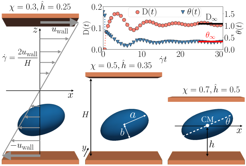
Figure 1: We consider a single drop under simple shear flow, i.e., confined in a channel with two walls placed at distance $H$ that move with velocity $u_{w}(x,y,z=\pm H/2)=(\pm u_{\mathrm{wall}},0,0)$. We vary the degree of confinement $\chi$, the drop relative height $\hat{h}$, the Boussinesq (Bq) and capillary (Ca) numbers. For each parameter combination, we measure the time-evolution of the drop deformation $\mathrm{D}(t)$ and the inclination angle $\theta(t)$ (upper-right panel). The deformation is computed as D$(t)=(a(t)-b(t))/(a(t)+b(t))$, where $a$ and $b$ are the drop main axes in the $xz$ plane. The steady-state value D_∞ (solid black line) and $\theta_{\infty}$ (solid red line) are then considered. Data in the upper-right panel correspond to the situation with Ca$=0.33$, Bq$=40$, $\chi=0.7$, and $\hat{h}=0.5$.

In this Letter, we present a unified analytical prediction for the steady-state deformation and inclination angle of a confined/unconfined drop with/without interface viscosity. At this level of investigation, numerical simulations are crucial in exploring all possible parameter combinations with precise control, which is challenging in experiments.

Specifically, we perform immersed boundary – lattice Boltzmann numerical simulations of a single confined drop under shear flow [34, 35]. Such a hybrid method has largely been employed to simulate the dynamics of drops [32, 33, 36, 37] and capsules [38, 39, 12] with and without interface viscosity. In particular, our in-house GPU code has already been extensively validated [33, 40, 41, 36] (see these works for further details). We consider a drop of radius $R$ immersed in a fluid with viscosity $\mu$, characterized by a viscosity ratio between inner and outer fluid viscosity $\lambda$, surface tension $\sigma$, and interface viscosity $\mu_{\mbox{\scriptsize int}}$. The drop is placed between two walls in the $xy$ plane, located at $z=\pm H/2$ and separated by a distance $H$. The drop’s CM is fixed at a distance $h$ from the lower wall. We apply a shear rate $\dot{\gamma}=2u_{\mathrm{wall}}/H$ by moving the walls with a velocity $u_{w}(x,y,z=\pm H/2)=(\pm u_{\mathrm{wall}},0,0)$ (see Fig. 1). The Reynolds number $\text{Re}=\rho\dot{\gamma}R^{2}/\mu$ keeps values smaller than $10^{-2}$ to avoid inertial effects. We measure the drop steady-state deformation $\text{D}_{\infty}$ and the inclination angle $\theta_{\infty}$ by varying the capillary number $\text{Ca}=\dot{\gamma}\mu R/\sigma$, the Boussinesq number $\text{Bq}=\mu_{\mbox{\scriptsize int}}/R\mu$, the degree of confinement $\chi=2R/H$, and the relative height of the drop’s CM $\hat{h}=h/H$. In this work, the drop is modeled via a triangular mesh with $1.8\times 10^{4}$ faces and radius $R=20\ \delta x$, with $\delta x=1$ being the lattice spacing. The fluid domain is a three-dimensional rectangular box with sizes $\text{L}_{\mbox{\scriptsize x}}=\text{L}_{\mbox{\scriptsize y}}=128\ \delta x$ and $\text{L}_{\mbox{\scriptsize z}}=H$, which varies to explore different $\chi$.

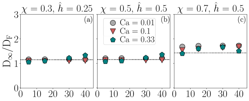
Figure 2: For three representative combinations of $\chi$ and $\hat{h}$ with $\lambda=1$, we show data for the measured steady-state value of the drop deformation D_∞, normalized with the corresponding value of D_F, as a function of Bq. Dotted black line reports the corresponding value of the function $\Psi$. Different colors/symbols correspond to different values of Ca.

To derive a unified analytical prediction for steady-state drop deformation and inclination angle under shear flow, we start considering the deformation theory from Shapira & Haber [24] for confined pure drops, which reads $\text{D}_{\mbox{\scriptsize SH}}(\lambda,\hat{h},\chi,\text{Ca})=\text{D}_{\mbox{\scriptsize T}}(\lambda,\text{Ca})\Psi(\lambda,\hat{h},\chi)$, where $\text{D}_{\mbox{\scriptsize T}}(\lambda,\text{Ca})=\text{Ca}(19\lambda+16)/(16\lambda+16)$ is the Taylor deformation for an unconfined pure drop [13], and $\Psi(\lambda,\hat{h},\chi)=1+C_{s}(\hat{h})(\chi/2)^{3}(1+2.5\lambda)/(1+\lambda)$ is a function accounting for the degree of confinement. The coefficient $C_{s}(\hat{h})$  represents the shape factor [24]. It is worth noting that for $\chi=0$ (unconfined drop), $\Psi=1$ and $\text{D}_{\mbox{\scriptsize SH}}=\text{D}_{\mbox{\scriptsize T}}$, as expected.

To extend the result by Shapira & Haber to include the effect of interface viscosity, we first replace $\text{D}_{\mbox{\scriptsize T}}(\lambda,\text{Ca})$ with the deformation $\text{D}_{\mbox{\scriptsize F}}(\lambda,\text{Ca},\text{Bq})$ computed by Flumerfelt for an unconfined drop with interface viscosity [29] (see Eq. (7a) in Appendix), thus obtaining $\mbox{D}(\lambda,\hat{h},\chi,\text{Ca},\text{Bq})=\text{D}_{\mbox{\scriptsize F}}(\lambda,\text{Ca},\text{Bq})\Psi(\lambda,\hat{h},\chi)$. Indeed, the latter must recover Flumerfelt’s result in the case $\chi=0$. To verify that $\Psi(\lambda,\hat{h},\chi)$ does not depend on the interface viscosity, we performed simulations with $\lambda=1$ for different combinations of Ca, $\chi$, and $\hat{h}$ and we report the ratio $\text{D}_{\infty}/\text{D}_{\mbox{\scriptsize F}}$ as a function of Bq in Fig. 2. The black-dashed line represents $\Psi(\lambda,\hat{h},\chi)$. Our analysis confirms the assumption that $\Psi$ does not depend on Bq. A small dependence only shows for high capillary numbers ($\text{Ca}=0.33$). As already observed experimentally for pure drops [25], we notice that $\Psi$ slightly underestimates the measured values when the confinement is high (panel (c)).

As a result, we obtain a unified analytical expression for the steady-state deformation of a confined drop with interface viscosity:

$$\mbox{D}(\lambda,\hat{h},\chi,\text{Ca},\text{Bq})=\frac{19\lambda+16+32\text{Bq}}{(16\lambda+16+32\text{Bq})\sqrt{\text{Ca}^{-2}+\frac{19F}{20}(\lambda+2\text{Bq})}}\left[1+C_{s}(\hat{h})\frac{\chi^{3}}{8}\frac{1+2.5\lambda}{1+\lambda}\right]\ ,$$ (1)

with $F$ reported in Appendix (see Eq. (8)), and the first factor on the r.h.s being $\text{D}_{\mbox{\scriptsize F}}$ (see Eq. (7a) in Appendix). In the two limit cases of an unconfined drop with interface viscosity ($\chi=0$, $\text{Bq}>0$) and a confined pure drop ($\chi>0$, $\text{Bq}=0$), Eq. (1) exactly recovers Flumerfelt’s and Shapira & Haber’s predictions, respectively.

To further validate Eq. (1), we compare it with numerical simulation data. Since drop deformation in Eq.(1) depends on five parameters ($\lambda$, $\hat{h}$, $\chi$, Ca, Bq), we start by fixing $\lambda=1$ and varying the remaining parameters. We do not show data in either the case of an unconfined drop with interface viscosity or the confined pure drop because results have already been widely explored [29, 24].

Fig. 3 reports the measured steady-state deformation $\text{D}_{\infty}$ as a function of Bq for different drop relative height $\hat{h}$ (columns) and different degrees of confinement $\chi$ (rows). Symbols represent numerical simulation data, while solid lines show the theoretical prediction given by Eq. (1). The overall effect of increasing confinement is to enhance the drop deformation, as already known for the pure drop [24]; on the other hand, the effect of interface viscosity is to reduce the deformation [29]. The combination of both ingredients holds the same qualitative scenario. Numerical results and analytical predictions are in good agreement, showing a slight difference for the combination of strong confinement ($\chi=0.7$), large values of interface viscosity ($\text{Bq}\geq 30$), and low relative drop height ($\hat{h}=0.35$). Such differences have also been observed experimentally for pure drops [25, 43], where experiments for high values of capillary number ($\text{Ca}\approx 0.3$) and high degrees of confinement ($\chi>0.5$) show that the prediction by Shapira & Haber underestimate the measured values. Notice that simulation data for the case $\chi=0.7$ and $\hat{h}=0.25$ does not exist because the distance $h$ would be smaller than $R$ (see Fig. 1). Further, we remark that the correction that our model provides on the already existing theories is sensible: indeed, dashed lines in Fig. 3 refer to Flumerfelt’s prediction ($\text{D}_{\mbox{\scriptsize F}}$) for the unconfined drop with interface viscosity. As expected, Eq. (1) is close to $\text{D}_{\mbox{\scriptsize F}}$ only for small values of $\chi$. To visually capture the effect of both interface viscosity and confinement on drop shape, bottom panels (1-8) of Fig. 3 show snapshots of the steady-state configurations for selected and relevant combinations of $\text{Ca},\hat{h}$ and $\chi$, spanning from the less confined drop with a small interface viscosity (panel (1)) to the most confined case with the highest considered value of Bq (panel (8)). The effect of interface viscosity can be appreciated by comparing left ($\text{Bq}=5$) and right ($\text{Bq}=40$) panels, while the effect of the proximity to the wall is reflected in a not-symmetric drop shape (panels (3-4)). This asymmetry is mitigated by the effect of interface viscosity.

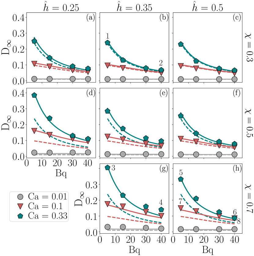
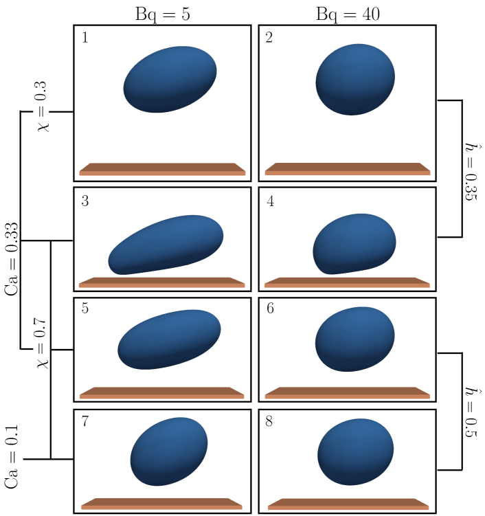
Figure 3: Top panels: Measured steady-state value of the drop deformation D_∞ as a function of Bq for $\lambda=1$. Symbols show simulation data, while solid and dotted lines correspond to Eq. (1) and Flumerfelt’s prediction (Eq. (7a)), respectively. Different colors/symbols correspond to different values of Ca. Bottom panels: steady-state shape of droplets undergoing parameters’ combination that are marked in top panels with index $i=1,\dots,8$.

We now move our attention to the derivation of an analytical prediction for the drop inclination angle. With this aim, as a starting point, we consider the model proposed by Maffettone & Minale (MM) [44], where the shape evolution of an unconfined pure ellipsoidal drop ($\chi=0$, $\text{Bq}=0$) is described in terms of two functions, $f_{1}(\lambda)=f_{1}^{(\mbox{\tiny MM})}=40(\lambda+1)/[(2\lambda+3)(19\lambda+16)]$ and $f_{2}(\lambda)=f_{2}^{(\mbox{\tiny MM})}=5/(2\lambda+3)$, which have been chosen to recover the first-order expansion in Ca of the shape-evolution equation computed by Rallison [16]. In the limit of small Ca, the steady-state deformation $\mathrm{D}$ and the inclination angle $\theta$ can be computed as $\mbox{D}=\text{Ca}f_{2}/2f_{1}$ and $\tan(2\theta)=f_{1}/\text{Ca}$, respectively [44]. To include the effect of interface viscosity, we match $f_{1}$ and $f_{2}$ with the first-order expansion computed by Narsimhan [10], which is analogous to Rallison’s calculations but accounting for the interface viscosity, thus obtaining $f_{1}=f_{1}^{(\mbox{\tiny N})}$ and $f_{2}=f_{2}^{(\mbox{\tiny N})}$ (see Eqs. (6) in Appendix). To also add the effect of confinement, we follow Minale’s approach [43] and we extend $f_{i}$ as $f_{1}=f_{1}^{(\mbox{\tiny N})}/\psi_{1}(\lambda,\hat{h},\chi,\text{Bq})$ and $f_{2}=f_{2}^{(\mbox{\tiny N})}\psi_{2}(\lambda,\hat{h},\chi,\text{Bq})$, with $\psi_{i}=1+C_{s}(\hat{h})(\chi/2)^{3}\tilde{f}_{i}(\lambda,\text{Bq})$ and $i=1,2$. Hence, we first write the first-order expansion in Ca of Eq. (1) as:

$$\small\mbox{D}^{(1)}=\text{Ca}\frac{19\lambda+16+32\text{Bq}}{16\lambda+16+32\text{Bq}}\left[1+C_{s}(\hat{h})\frac{\chi^{3}}{8}\frac{1+2.5\lambda}{1+\lambda}\right];$$ (2)

then, we compute the deformation for small Ca as $D=\text{Ca}f_{2}/2f_{1}$, thus obtaining ($\mathcal{O}(\chi^{6})$ have been neglected):

$$\small\frac{f_{2}}{2f_{1}}=\frac{f_{2}^{(\mbox{\tiny N})}}{2f_{1}^{(\mbox{\tiny N})}}\psi_{1}\psi_{2}=\frac{f_{2}^{(\mbox{\tiny N})}}{2f_{1}^{(\mbox{\tiny N})}}\left[1+C_{s}(\hat{h})\frac{\chi^{3}}{8}(\tilde{f}_{1}+\tilde{f}_{2})\right]\ .$$ (3)

By comparing Eq. (3) with Eq. (2), it is straightforward to see that $\tilde{f}_{1}+\tilde{f}_{2}=(1+2.5\lambda)/(1+\lambda)$. This implies that, once $\tilde{f}_{2}$ is determined, $\tilde{f}_{1}$ is fixed. Finally, we extend Minale’s results by assuming the most straightforward dependence of $\tilde{f}_{i}$ on Bq, i.e., $\tilde{f}_{2}(\lambda,\text{Bq})=-(10-9\lambda+k_{1}\text{Bq})/(12+\lambda+k_{2}\text{Bq})$, with $k_{1}$ and $k_{2}$ being two parameters to be fitted with experimental or numerical results [43]. By fitting the numerical values for drop deformation and inclination angle, we found $k_{1}=-10$ and $k_{2}=7/2$, leading to the final form of $\tilde{f}_{i}$:

$$\tilde{f_{1}}(\lambda,\text{Bq}) =\frac{22+32\lambda-\frac{13}{2}\lambda^{2}-\frac{1}{4}\text{Bq}(26+5\lambda)}{12+13\lambda+\lambda^{2}+\frac{7}{2}\text{Bq}(1+\lambda)}\ ,$$ (4a)

$$\tilde{f}_{2}(\lambda,\text{Bq}) =-\frac{10-9\lambda-10\text{Bq}}{12+\lambda+\frac{7}{2}\text{Bq}}\ .$$ (4b)

We can now compute the inclination angle as:

$$\tan 2\theta=\frac{\left[40\left(\lambda+1\right)+80\text{Bq}\right](\psi_{1}\text{Ca})^{-1}}{\left(2\lambda+3\right)\left(19\lambda+16\right)+\text{Bq}(32\text{Bq}+98\lambda+112)}\ .$$ (5)

When $\text{Bq}=0$, Minale’s results are retrieved.

In Fig. 4, we compare the prediction from Eq. (5) with numerical simulation data. Unlike the deformation, the effect of the confinement is not pronounced, as emerged from the marginal difference between Eq. (5) (solid line) and Flumerfelt’s results (Eq. (7b), dashed lines). However, it is interesting to notice that a strong non-linear behavior emerges for large values of Ca, regardless of the degree of confinement: for a given Ca (e.g., $\text{Ca}=0.33$), we observe a non-monotonic behavior of $\theta$ as Bq increases. However, this result is not surprising since we derived Eq. (5) in the limit of small Ca. Furthermore, this behavior is qualitatively in agreement with numerical simulations of other works concerning unconfined drops with interface viscosity [33] and unconfined capsules with membrane viscosity [45].

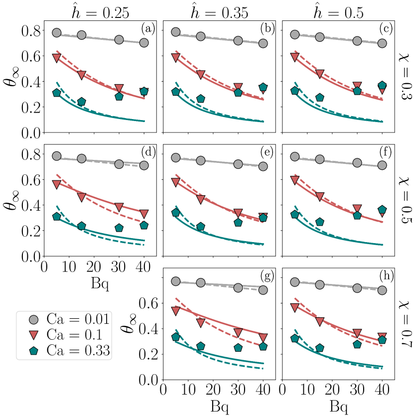
Figure 4: Steady-state value of the drop inclination angle $\theta_{\infty}$ as a function of Bq for $\lambda=1$. Symbols show simulation data, while solid and dotted lines correspond to Eq. (5) and Flumerfelt’s prediction (Eq. (7b)), respectively. Different colors/symbols correspond to different values of Ca.

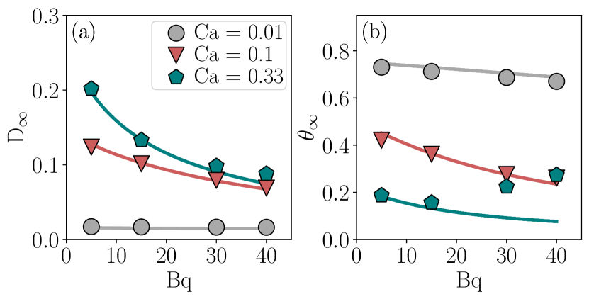
Figure 5: Steady-state value of the drop deformation D_∞ (panel (a)) and $\theta_{\infty}$ (panel (b)) as a function Bq for a value of $\lambda=5.2$, $\chi=0.7$, and $\hat{h}=0.5$. Symbols show simulation data, while solid lines correspond to predictions from Eq. (1) (panel (a)) and Eq. (5) (panel (b)). Different colors/symbols correspond to different values of Ca.

All results hitherto discussed refer to the case of $\lambda=1$. To prove the robustness of the unified analytical expressions for both D (Eq. (1)) and $\theta$ (Eq. (5)), we also explore a situation with $\lambda=5.2$, which is usually encountered in experiments [43, 26]. In Fig. 5, $\text{D}_{\infty}$ (panel (a)) and $\theta_{\infty}$ (panel (b)) are reported as functions of Bq for the most confined simulated case (i.e., $\chi=0.7$ and $\hat{h}=0.5$). While $\text{D}_{\infty}$ shows a perfect agreement between simulation data and Eq. (1), $\theta_{\infty}$ behaves as in Fig. 4, with a good agreement with Eq. (5) for small values of Ca and a misalignment for $\text{Ca}=0.33$. This result further confirms the validity of our analytical predictions.

In conclusion, in this Letter, we fill the literature blanks concerning the estimation of steady-state behavior of drop under simple shear flow by presenting a unified analytical prediction describing the deformation (Eq. (1)) and inclination angle ((5)) of a confined/unconfined drop with/without interface viscosity. Since there are no available experiments for this system, in order to validate the quality and robustness of the proposed predictions, we performed immersed boundary-lattice Boltzmann simulations, which have already been validated in a series of previous works [32, 33, 36, 37]. We also compared Eqs. (1) and (5) with the already known analytical predictions computed by Flumerfelt [29] for the unconfined drop with interface viscosity, showing that the accounting of confinement effects in Flumerfelt’s prediction is fundamental to quantitatively describe the correct deformation of a drop under these conditions. The robustness of our unified analytical predictions is strengthened by its application to different values of the drop viscosity ratio. We hope this result can open a new route to experiments of confined/unconfined drops with interface viscosity.

Acknowledgment

We thank L. Biferale and M. Sbragaglia for fruitful discussions. This work was supported by the Italian Ministry of University and Research (MUR) under the FARE program (No. R2045J8XAW), project “Smart-HEART”, and it has been carried out within the TEXTAROSSA project (G.A. H2020-JTI-EuroHPC-2019-1 No. 956831).

APPENDIX

Functions $f_{1}^{(\mbox{\tiny N})}$ and $f_{2}^{(\mbox{\tiny N})}$

To include the interface viscosity, one can match the values of $f_{1,2}$ with the first order expansion of Eq.(3.1) in Ref. [10], obtaining:

$$f_{1}^{(\mbox{\tiny N})} =\frac{40\left(\lambda+1\right)+80\text{Bq}}{\left(2\lambda+3\right)\left(19\lambda+16\right)+\text{Bq}(32\text{Bq}+98\lambda+112)}\ ,$$ (6a)

$$f_{2}^{(\mbox{\tiny N})} =5\frac{19\lambda+16+32\text{Bq}}{\left(2\lambda+3\right)\left(19\lambda+16\right)+\text{Bq}(32\text{Bq}+98\lambda+112)}\ .$$ (6b)

Flumerfelt’s prediction

The steady-state deformation $\text{D}_{\mbox{\scriptsize F}}$ and inclination angle $\theta_{\mbox{\scriptsize F}}$ predicted by Flumerfelt [29] are:

$$\text{D}_{\mbox{\scriptsize F}}(\lambda,\text{Ca},\text{Bq})=\\ =\frac{19\lambda+16+32\text{Bq}}{(16\lambda+16+32\text{Bq})\sqrt{\text{Ca}^{-2}+\frac{19F}{20}(\lambda+2\text{Bq})}}\ ,$$ (7a)

$$\theta_{\mbox{\scriptsize F}}(\lambda,\text{Ca},\text{Bq})=\\ =\frac{\pi}{4}-\frac{1}{2}\arctan\left(\frac{19F}{20}(\lambda+2\text{Bq})\text{Ca}\right)\ ,$$ (7b)

with

$$F=1-\frac{9\lambda+18\text{Bq}-2}{8(\lambda+2\text{Bq})^{2}}\ .$$ (8)

References

- Kim and Greenburg [2004] H. W. Kim and A. G. Greenburg, Artificial oxygen carriers as red blood cell substitutes: a selected review and current status, Artificial Organs 28, 813 (2004).
- Gao and Zhang [2015] W. Gao and L. Zhang, Engineering red-blood-cell-membrane–coated nanoparticles for broad biomedical applications, AIChE Journal 61, 738 (2015).
- Xia et al. [2019] Q. Xia, Y. Zhang, Z. Li, X. Hou, and N. Feng, Red blood cell membrane-camouflaged nanoparticles: a novel drug delivery system for antitumor application, Acta Pharmaceutica Sinica B 9, 675 (2019).
- Quintero [2002] L. Quintero, An overview of surfactant applications in drilling fluids for the petroleum industry, Journal of Dispersion Science and Technology 23, 393 (2002).
- Zolfaghari et al. [2016] R. Zolfaghari, A. Fakhru’l-Razi, L. C. Abdullah, S. S. Elnashaie, and A. Pendashteh, Demulsification techniques of water-in-oil and oil-in-water emulsions in petroleum industry, Separation and Purification Technology 170, 377 (2016).
- Ofori and Hsieh [2012] J. A. Ofori and Y.-H. P. Hsieh, The use of blood and derived products as food additives, Food Additive 13, 229 (2012).
- Tan and McClements [2021] C. Tan and D. J. McClements, Application of advanced emulsion technology in the food industry: A review and critical evaluation, Foods 10, 812 (2021).
- Udayakumar et al. [2021] G. P. Udayakumar, S. Muthusamy, B. Selvaganesh, N. Sivarajasekar, K. Rambabu, F. Banat, S. Sivamani, N. Sivakumar, A. Hosseini-Bandegharaei, and P. L. Show, Biopolymers and composites: Properties, characterization and their applications in food, medical and pharmaceutical industries, Journal of Environmental Chemical Engineering 9, 105322 (2021).
- Guido and Villone [1998] S. Guido and M. Villone, Three-dimensional shape of a drop under simple shear flow, Journal of Rheology 42, 395 (1998).
- Narsimhan [2019] V. Narsimhan, Shape and rheology of droplets with viscous surface moduli, Journal of Fluid Mechanics 862, 385 (2019).
- Aouane et al. [2021] O. Aouane, A. Scagliarini, and J. Harting, Structure and rheology of suspensions of spherical strain-hardening capsules, Journal of Fluid Mechanics 911, A11 (2021).
- Guglietta et al. [2023] F. Guglietta, F. Pelusi, M. Sega, O. Aouane, and J. Harting, Suspensions of viscoelastic capsules: effect of membrane viscosity on transient dynamics, Journal of Fluid Mechanics 971, A13 (2023).
- Taylor [1932] G. I. Taylor, The viscosity of a fluid containing small drops of another fluid, Proceedings of the Royal Society of London. Series A, Containing Papers of a Mathematical and Physical Character 138, 41 (1932).
- Taylor [1934] G. I. Taylor, The formation of emulsions in definable fields of flow, Proceedings of the Royal Society of London. Series A, Containing Papers of a Mathematical and Physical Character 146, 501 (1934).
- Chaffey and Brenner [1967] C. E. Chaffey and H. Brenner, A second-order theory for shear deformation of drops, Journal of Colloid and Interface Science 24, 258 (1967).
- Rallison [1980] J. Rallison, Note on the time-dependent deformation of a viscous drop which is almost spherical, Journal of Fluid Mechanics 98, 625 (1980).
- Barthès-Biesel and Acrivos [1973] D. Barthès-Biesel and A. Acrivos, Deformation and burst of a liquid droplet freely suspended in a linear shear field, Journal of Fluid Mechanics 61, 1 (1973).
- Torza et al. [1972] S. Torza, R. Cox, and S. Mason, Particle motion in sheared suspensions. xxvii. transient and steady deformation and burst of liquid drops, Journal of Colloid and Interface Science 38, 395 (1972).
- Phillips et al. [1980] W. J. Phillips, R. W. Graves, and R. W. Flumerfelt, Experimental studies of drop dynamics in shear fields: Role of dynamic interfacial effects, Journal of Colloid and Interface Science 76, 350 (1980).
- Grace [1982] H. P. Grace, Dispersion phenomena in high viscosity immiscible fluid systems and application of static mixers as dispersion devices in such systems, Chemical Engineering Communications 14, 225 (1982).
- Gupta and Sbragaglia [2014] A. Gupta and M. Sbragaglia, Deformation and breakup of viscoelastic droplets in confined shear flow, Physical Review E 90, 023305 (2014).
- Komrakova et al. [2014] A. Komrakova, O. Shardt, D. Eskin, and J. Derksen, Lattice boltzmann simulations of drop deformation and breakup in shear flow, International Journal of Multiphase Flow 59, 24 (2014).
- Megias-Alguacil et al. [2005] D. Megias-Alguacil, K. Feigl, M. Dressler, P. Fischer, and E. J. Windhab, Droplet deformation under simple shear investigated by experiment, numerical simulation and modeling, Journal of Non-Newtonian Fluid Mechanics 126, 153 (2005).
- Shapira and Haber [1990] M. Shapira and S. Haber, Low Reynolds number motion of a droplet in shear flow including wall effects, International Journal of Multiphase Flow 16, 305 (1990).
- Sibillo et al. [2006] V. Sibillo, G. Pasquariello, M. Simeone, V. Cristini, and S. Guido, Drop Deformation in Microconfined Shear Flow, Physical Review Letters 97, 054502 (2006).
- Vananroye et al. [2007] A. Vananroye, P. Van Puyvelde, and P. Moldenaers, Effect of confinement on the steady-state behavior of single droplets during shear flow, Journal of Rheology 51, 139 (2007).
- Guido [2011] S. Guido, Shear-induced droplet deformation: Effects of confined geometry and viscoelasticity, Current Opinion in Colloid & Interface Science 16, 61 (2011).
- Vananroye et al. [2008] A. Vananroye, P. J. Janssen, P. D. Anderson, P. Van Puyvelde, and P. Moldenaers, Microconfined equiviscous droplet deformation: Comparison of experimental and numerical results, Physics of Fluids 20, 013101 (2008).
- Flumerfelt [1980] R. W. Flumerfelt, Effects of dynamic interfacial properties on drop deformation and orientation in shear and extensional flow fields, Journal of Colloid and Interface Science 76, 330 (1980).
- Pozrikidis [1994] C. Pozrikidis, Effects of surface viscosity on the finite deformation of a liquid drop and the rheology of dilute emulsions in simple shearing flow, Journal of Non-Newtonian Fluid Mechanics 51, 161 (1994).
- Gounley et al. [2016] J. Gounley, G. Boedec, M. Jaeger, and M. Leonetti, Influence of surface viscosity on droplets in shear flow, Journal of Fluid Mechanics 791, 464–494 (2016).
- Li and Zhang [2019] P. Li and J. Zhang, A finite difference method with subsampling for immersed boundary simulations of the capsule dynamics with viscoelastic membranes, International Journal for Numerical Methods in Biomedical Engineering 35, e3200 (2019).
- Guglietta et al. [2020] F. Guglietta, M. Behr, L. Biferale, G. Falcucci, and M. Sbragaglia, On the effects of membrane viscosity on transient red blood cell dynamics, Soft Matter 16, 6191 (2020).
- Benzi et al. [1992] R. Benzi, S. Succi, and M. Vergassola, The lattice Boltzmann equation: theory and applications, Physics Reports 222, 145 (1992).
- Krüger et al. [2017] T. Krüger, H. Kusumaatmaja, A. Kuzmin, O. Shardt, G. Silva, and E. M. Viggen, The lattice Boltzmann method, Springer International Publishing 10, 4 (2017).
- Taglienti et al. [2023] D. Taglienti, F. Guglietta, and M. Sbragaglia, Reduced model for droplet dynamics in shear flows at finite capillary numbers, Physical Review Fluids 8, 013603 (2023).
- Pelusi et al. [2023] F. Pelusi, F. Guglietta, M. Sega, O. Aouane, and J. Harting, A sharp interface approach for wetting dynamics of coated droplets and soft particles, Physics of Fluids 35, 082126 (2023).
- Krüger et al. [2011] T. Krüger, F. Varnik, and D. Raabe, Efficient and accurate simulations of deformable particles immersed in a fluid using a combined immersed boundary lattice Boltzmann finite element method, Computers & Mathematics with Applications 61, 3485 (2011).
- Krüger et al. [2014] T. Krüger, B. Kaoui, and J. Harting, Interplay of inertia and deformability on rheological properties of a suspension of capsules, Journal of Fluid Mechanics 751, 725 (2014).
- Guglietta et al. [2021a] F. Guglietta, M. Behr, G. Falcucci, and M. Sbragaglia, Loading and relaxation dynamics of a red blood cell, Soft Matter 17, 5978 (2021a).
- Guglietta et al. [2021b] F. Guglietta, M. Behr, L. Biferale, G. Falcucci, and M. Sbragaglia, Lattice Boltzmann simulations on the tumbling to tank-treading transition: effects of membrane viscosity, Philosophical Transactions of the Royal Society A: Mathematical, Physical and Engineering Sciences 379, 20200395 (2021b).
- Note [1] The values of used in this work are , and and are taken from Ref. [24].
- Minale [2008] M. Minale, A phenomenological model for wall effects on the deformation of an ellipsoidal drop in viscous flow, Rheologica Acta 47, 667 (2008).
- Maffettone and Minale [1998] P. Maffettone and M. Minale, Equation of change for ellipsoidal drops in viscous flow, Journal of Non-Newtonian Fluid Mechanics 78, 227 (1998).
- Yazdani and Bagchi [2013] A. Yazdani and P. Bagchi, Influence of membrane viscosity on capsule dynamics in shear flow, Journal of Fluid Mechanics 718, 569–595 (2013).