Conformal Predictive Systems Under Covariate Shift

Abstract

Conformal Predictive Systems (CPS) offer a versatile framework for constructing predictive distributions, allowing for calibrated inference and informative decision-making. However, their applicability has been limited to scenarios adhering to the Independent and Identically Distributed (IID) model assumption. This paper extends CPS to accommodate scenarios characterized by covariate shifts. We therefore propose Weighted CPS (WCPS), akin to Weighted Conformal Prediction (WCP), leveraging likelihood ratios between training and testing covariate distributions. This extension enables the construction of nonparametric predictive distributions capable of handling covariate shifts. We present theoretical underpinnings and conjectures regarding the validity and efficacy of WCPS and demonstrate its utility through empirical evaluations on both synthetic and real-world datasets. Our simulation experiments indicate that WCPS are probabilistically calibrated under covariate shift.

Keywords Conformal prediction  $\cdot$ Conformal predictive systems  $\cdot$ Predictive distributions  $\cdot$ Regression  $\cdot$ Covariate shift

1 Introduction

Conformal Predictive Systems (CPS) are a relatively recent development in Conformal Prediction (CP) (Vovk et al., 2019, 2020a). CPS construct predictive distributions by arranging p-values into a nonparametric probability distribution. This distribution satisfies a finite-sample property of validity under the Independent and Identically Distributed (IID) model, i.e., the observations are produced independently from the same probability measure. CPS can be seen as a generalization of point and conformal regressors since they can easily produce point predictions and prediction intervals by leveraging the generated predictive distributions. They allow for more informative and trustworthy decision-making (Vovk et al., 2018).

In alignment with the inception of conformal regressors, several adaptations, and enhancements have emerged in the literature after the initial work of Vovk et al. (2019). These include more computationally efficient variants  (Vovk et al., 2020a), adaptive versions (Vovk et al., 2020b; Boström et al., 2021; Johansson et al., 2023; Jonkers et al., 2024a), and proving the existence of universal consistent CPS  (Vovk, 2022).

The exchangeability assumption, which allows for provably valid inference for CP and is a weaker assumption than the IID assumption (Shafer and Vovk, 2008), and similarly, the IID assumption for CPS, are standard in machine learning. However, distributional shifts between training and inference data are common in time series, counterfactual inference, and machine learning for scientific discovery but violate these assumptions. While a growing amount of literature has been contributed to extending CP beyond the exchangeability assumptions (Tibshirani et al., 2019; Gibbs and Candes, 2021; Prinster et al., 2022; Yang et al., 2022; Gibbs and Candès, 2023), allowing (conservatively) valid inference under various types of distributional shifts, no contribution has been made towards extending CPS beyond the IID model. For example, in treatment effect estimation, this extension could allow calibrated predictive distribution beyond the randomized trial setting (Jonkers et al., 2024b), as in a nonrandomized setting, the covariate distributions for treated and control subjects differ from the target population. Therefore, this work extends CPS beyond the IID model by proposing weighted CPS that constructs valid nonparametric predictive distributions for problems where the covariate distributions of the training and testing data differ, assuming their likelihood ratio is known or can be estimated.

The remainder of this paper is organized as follows: in Section 2, we will give some background and restate propositions around CP, CPS, and covariate shifts. Section 3 presents our modification of CPS to deal with covariate shift, followed by Section 4 and Section 5, which discusses and summarizes the main findings, respectively.

2 Background

Let $\textbf{Z}:=\textbf{X}\times\mathbb{R}$ be the observation space where each observation $z=(x,y)\in\textbf{Z}$ consist of an object $x\in\textbf{X}$ and its label $y\in\mathbb{R}$. Additionaly, lets $z_{1},...,z_{n}$ be the training sequence and $z_{n+1}=(x_{n+1},y_{n+1})$ be the test observation.

2.1 Conformal Prediction

Conformal Prediction (CP) (Vovk et al., 2022) is a model-agnostic and distribution-free framework that allows us to give an implicit confidence estimate in a prediction by generating prediction sets at a specific significance level $\alpha$. The framework provides (conservatively) valid non-asymptotic confidence predictors under the exchangeability assumption. This exchangeability assumption assumes that the training/calibration data should be exchangeable with the test data. The prediction sets in CP are formed by comparing nonconformity scores of examples that quantify how unusual a predicted label is, i.e., these scores measure the disagreement between the prediction and the actual target.

To do so, we define a prediction interval $\hat{C}(x_{n+1})$, for test object $x_{n+1}\in\mathbf{X}$, by calculating following conformity scores $R_{i}^{y}$, based on conformity measure $A$, for each $y\in\mathbb{R}$:

$$R_{i}^{y}=A(z_{i},z_{1:n\setminus i}\cup(x_{n+1},y)),\quad i=1,...,n$$ (1)

and

$$R_{n+1}^{y}=A((x_{n+1},y),z_{1:n}).$$ (2)

The label $y$ is then included in prediction interval $\hat{C}(x_{n+1})$ if,

$$\frac{|i=1,...,n+1:R_{i}^{y}\geq R_{n+1}^{y}|}{n+1}>\alpha$$ (3)

The procedure above is referred to as full or transductive conformal prediction and is computationally heavy. Therefore, Papadopoulos et al. (2002) proposed a more applicable variant of full CP, called Inductive or split CP (ICP). ICP is computationally less demanding and allows the use of CP in conjunction with machine learning algorithms, such as neural networks and tree-based algorithms. ICP starts by splitting the training sequence $(x,y)=\{(x_{1},y_{1}),...,(X_{n},y_{n})\}$ into a proper training sequence $\{(x_{1},y_{1}),...,(x_{m},y_{m})\}$ and a calibration sequence $\{(x_{m+1},y_{m+1}),...,(x_{n},y_{n})\}$. The proper training sequence is used to train a regression model. We then generate nonconformity scores $R_{i}$ for $(x_{i},y_{i})$ with $i=m+1,...,n$ from the calibration set, such as for the absolute error, $R_{i}=|y_{i}-\hat{y}_{i}|$. These nonconformity scores are sorted in descending order: $R^{*}_{1},...,R^{*}_{n-m}$. For a new test object $x_{n+1}$, point prediction $\hat{y}_{n+1}$, and a desired target coverage of $1-\alpha$, ICP outputs the following prediction interval:

$$[\hat{y}_{n+1}-R^{*}_{s},\hat{y}_{n+1}+R^{*}_{s}]$$ (4)

where $s=\lfloor\alpha(n-m+1)\rfloor$.

2.2 Covariate Shift

A covariate shift is a distributional shift where the test object $(x_{n+1},y_{n+1})$ is differently distributed, i.e. $x_{n+1}\sim\tilde{P}_{X}$, than the training data $z_{i}=(x_{i},y_{i}),i=1,...,n$ where $x_{i}\sim P_{X}$, thus $\tilde{P}_{X}\neq P_{X}$. However, the relationship between inputs and labels remains fixed.

$$\begin{split}(x_{i},y_{i})\mathop{\sim}\limits^{\mathrm{iid}}P&=P_{X}\times P_{Y|X},\quad i=1,...,n\\ (x_{n+1},y_{n+1})\sim\tilde{P}&=\tilde{P}_{X}\times P_{Y|X}\end{split}$$ (5)

2.3 Weighted Conformal Prediction

Tibshirani et al. (2019) was one of the first works to extend conformal prediction beyond the exchangeability assumption to deal with covariate shifts. Specifically, they propose Weighted Conformal Prediction (WCP) to deal with covariate shifts where the likelihood ratio between the training $P_{X}$ and test $\tilde{P}_{X}$ covariate distributions is known. In WCP, the empirical distribution of nonconformity scores at the training points gets reweighted, and thus each nonconformity score $R_{i}$ gets weighted by a probability $p_{i}^{w}(x)$ proportional to the likelihood ratio $w(x_{i})=\frac{d\tilde{P}_{X}(x_{i})}{P_{X}(x_{i})}$:

$$p_{i}^{w}(x) =\frac{w(x_{i})}{\sum_{j=1}^{n}w(x_{j})+w(x)},\qquad i=1,...,n,$$ (6)

$$p_{n+1}^{w}(x) =\frac{w(x)}{\sum_{j=1}^{n}w(x_{j})+w(x)}.$$ (7)

This results in an adjusted empirical distribution of nonconformity scores depicted in Table 1.

Table 1: Empirical distribution of nonconformity scores ($\delta_{a}$ denotes a point mass at $a$).

Regular	Weighted
$\frac{1}{n+1}\sum_{i=1}^{n}\delta_{R_{i}}+\frac{1}{n+1}\delta_{\infty}$	$\sum_{i=1}^{n}p_{i}^{w}(x)\delta_{R_{i}}+p_{n+1}^{w}(x)\delta_{\infty}$

Tibshirani et al. (2019) showed that the validity of WCP remains even for the computational less-demanding split conformal prediction. However, this all does not come for free; we are reducing the sample size by weighting nonconformity scores and consequentially losing some reliability, i.e., variability in empirical coverage, compared to CP without covariate shift and the same number of samples. Tibshirani et al. (2019) pointed out a popular heuristic from the covariate shift literature (Gretton et al., 2008; Reddi et al., 2015) to determine the effective sample size $\hat{n}$ of $X_{1},...,X_{n}$ training points, and a likelihood ratio $w$:

$$\hat{n}=\frac{[\sum_{i=1}^{n}|w(x_{i})|]^{2}}{\sum_{i=1}^{n}|w(x_{i})|^{2}}=\frac{||w(x_{1:n})||_{1}^{2}}{||w(x_{1:n})||_{2}^{2}}$$ (8)

where $w(x_{1:n})=(w(x_{1}),...,w(x_{n}))$. Note that it is possible to learn the likelihood ratio $w(x_{i})=\frac{d\tilde{P}_{X}(x_{i})}{P_{X}(x_{i})}$ between training and test covariate distribution, as showed by Tibshirani et al. (2019), if it is reasonably accurate.

2.4 Conformal Predictive Systems

Conformal Predictive Systems (CPS) allow the construction of predictive distributions by extending upon full CP. CPS produces conformal predictive distributions by arranging p-values into a probability distribution function (Vovk et al., 2019). These p-values are created with the help of specific types of conformity measures. Vovk et al. (2019) defines a CPS as a function that is both a conformal transducer (Definition 1) and a Randomized Predictive System (RPS) (Definition 2).

Definition 1 (Conformal Transducer, Vovk et al. (2022)).

The conformal transducer determined by a conformity measure $A$ is defined as,

$$Q(z_{1},...,z_{n},(x,y),\tau):=\sum_{i=1}^{n+1}[R_{i}^{y}<R_{n+1}^{y}]\frac{1}{n+1}+\sum_{i=1}^{n+1}[R_{i}^{y}=R_{n+1}^{y}]\frac{\tau}{n+1}$$

where $(z_{1},...,z_{n})$ is the training sequence, $\tau\in[0,1]$, $x_{n+1}$ is a test object, and for each label $y$ the corresponding conformity score $R_{i}^{y}$ is defined as

$$\begin{split}R_{i}^{y}&:=A(z_{1},...,z_{i-1},z_{i+1},...,z_{n},(x_{n+1},y),z_{i}),\qquad i=1,...,n\\ R_{n+1}^{y}&:=A(z_{1},...,z_{n},(x_{n+1},y)).\end{split}$$

Definition 2 (RPS, Vovk et al. (2019)).

A function $Q:\textbf{Z}^{n+1}\times[0,1]\rightarrow[0,1]$ is an RPS if it satisfies the following requirements:

• For each training sequence $(z_{1},...,z_{n})\in\textbf{Z}^{n}$ and test object $x\in\textbf{X}$, the function $Q(z_{1},...,z_{n},(x,y),\tau)$ is monotonically increasing both in $y$ and $\tau$. Put differently, for each $\tau\in[0,1]$, the function

  $$y\in\mathbb{R}\rightarrow Q(z_{1},...,z_{n},(x,y),\tau)$$

  is monotonically increasing, and for each $y\in\mathbb{R}$, the function

  $$\tau\in[0,1]\rightarrow Q(z_{1},...,z_{n},(x,y),\tau)$$

  is also monotonically increasing.

• For each $\tau,\tau^{\prime}\in[0,1]$ and each test object $x\in\textbf{X}$,

  $$Q(z_{1},...,z_{n},(x,y),\tau)>Q(z_{1},...,z_{n},(x,y^{\prime}),\tau^{\prime}),\qquad\text{if}\quad y>y^{\prime}$$

• For each training sequence $(z_{1},...,z_{n})\in\textbf{Z}^{n}$ and test object $x\in\textbf{X}$,

  $$\lim_{y\rightarrow-\infty}Q(z_{1},...,z_{n},(x,y),0)=0$$

  and

  $$\lim_{y\rightarrow\infty}Q(z_{1},...,z_{n},(x,y),1)=1$$

• As a function of random training observations $z_{1}\sim P,...,z_{n}\sim P$, and a random number $\tau\sim Uniform(0,1)$, all assumed to be independent, the distribution of Q is uniform:

  $$\forall\alpha\in[0,1]:\mathbb{P}\{Q(z_{1},...,z_{n},z_{n+1},\tau)\leq\alpha\}=\alpha$$

Definition 2 that defines an RPS is in verbatim from Vovk et al. (2019), except requirement R1.2, which is appended to the definition as we believe this is a requirement which is implicitly assumed by Vovk et al. (2019).

Note that a conformal transducer satisfies R2 by its validity property (see Proposition 2.11 in Vovk et al. (2022)). Additionally, in Vovk (2022) (Lemma 1), they show that a conformal transducer defined by a monotonic conformity measure $A$ is also an RPS and thus a CPS if $A$ follows the following three conditions:

• for all $n$, all training data sequences $(z_{1},...,z_{n})$, and all test objects $x_{n+1}$,

  $$\inf_{y}A(z_{1},...,z_{n},(x_{n+1},y))=\inf A_{n}$$ (9)

  $$\sup_{y}A(z_{1},...,z_{n},(x_{n+1},y))=\sup A_{n};$$ (10)

• for each n, the $\inf_{y}$ in Equation 9 is either attained for all $(z_{1},...,z_{n})$ and $x_{n+1}$, or not attained for any $(z_{1},...,z_{n})$ and $x_{n+1}$;

• for each n, the $\sup_{y}$ in Equation 10 is either attained for all $(z_{1},...,z_{n})$ and $x_{n+1}$, or not attained for any $(z_{1},...,z_{n})$ and $x_{n+1}$.

2.4.1 Split Conformal Predictive Systems

Like CP, CPS has been adapted and made more computationally efficient by building upon ICP, namely Split Conformal Predictive Systems (SCPS) (Vovk et al., 2020a). Here, the p-values are created by a split conformity measure that needs to be isotonic and balanced. A good and standard choice of split conformity measure, according to Vovk et al. (2020a), is a (normalized) residual. In Appendix A, we present and discuss, similarly as for CPS, definitions and propositions related to SCPS.

3 Weighted Conformal Predictive System

As WCP extends upon CP, we propose to reweigh the conformity scores with a probability $p_{i}^{w}(x)$ proportional to the likelihood ratio $w(x_{i})=\frac{d\tilde{P}_{X}(x_{i})}{P_{X}(x_{i})}$, to present a weighted conformal transducer where the output is defined by conformity measure $A$ and likelihood ratio $w(x)=\frac{d\tilde{P}_{X}(x)}{P_{X}(x)}$,

$$Q(z_{1},...,z_{n},\frac{d\tilde{P}}{P},(x,y),\tau):=\sum_{i=1}^{n+1}[R_{i}^{y}<R_{n+1}^{y}]p_{i}^{w}(x)+\sum_{i=1}^{n+1}[R_{i}^{y}=R_{n+1}^{y}]p_{i}^{w}(x)\tau$$ (11)

where $\tau$ is a random number sampled from a uniform distribution between 0 and 1. Note that under the absence of a covariate shift, the probability weights become equal, $p_{i}^{w}(x)=p^{w}_{n+1}=\frac{1}{n+1}$. In this scenario, the weighted conformal transducer (11) will become equivalent to a conformal transducer.

A function is a Weighted Conformal Predictive System (WCPS) if it is both a weighted conformal transducer and an RPS. To prove that under specific conformity measures $A$, e.g., monotonic conformity measures, a weighted conformal transducer is also an RPS, we need to prove Conjecture 1, i.e., that the weighted conformal transducer is probabilistically calibrated.

Conjecture 1.

Assume that

• $z_{i}=(x_{i},y_{i})\in\mathbf{X}\times\mathbb{R}$, $i=1,...,n$ are produced independently from $P=P_{X}\times P_{Y|X}$;

• $z_{n+1}=(x_{n+1},y_{n+1})\in\mathbf{X}\times\mathbb{R}$, is independently drawn from $\tilde{P}=\tilde{P}_{X}\times P_{Y|X}$;

• $\tilde{P}_{X}$ is absolutely continuous with respect to $P_{X}$;

• random number $\tau\sim Uniform(0,1)$;

• $z_{1:n}$, $z_{n+1}$, and $\tau$ to be independent.

Then the distribution of the weighted conformal transducer, defined by (11), is uniform:

$$\forall\alpha\in[0,1]:\mathbb{P}_{z_{1:n}\sim P,z_{n+1}\sim\tilde{P}}\{Q(z_{1},...,z_{n},\frac{d\tilde{P}}{P},z_{n+1},\tau)\leq\alpha\}=\alpha$$ (12)

We leave this proof for future work. However, if proven, Conjecture 2 can be easily proven by following the same procedure as the proof of Lemma 1 in Vovk (2022) using Conjecture 1 instead of the property of validity of a conformal transducer.

Conjecture 2 (Weighted Version of Lemma 1 in Vovk (2022)).

Suppose a monotonic conformity measure $A$ satisfies the following three conditions:

• for all $n$, all training data sequences $(z_{1},...,z_{n})$, and all test objects $x_{n+1}$,

  $$\inf_{y}A(z_{1},...,z_{n},(x_{n+1},y))=\inf A_{n}$$ (13)

  $$\sup_{y}A(z_{1},...,z_{n},(x_{n+1},y))=\sup A_{n};$$ (14)

• for each n, the $\inf_{y}$ in Equation 13 is either attained for all $(z_{1},...,z_{n})$ and $x_{n+1}$ or not attained for any $(z_{1},...,z_{n})$ and $x_{n+1}$;

• for each n, the $\sup_{y}$ in Equation 14 is either attained for all $(z_{1},...,z_{n})$ and $x_{n+1}$ or not attained for any $(z_{1},...,z_{n})$ and $x_{n+1}.$

Then, the weighted conformal transducer corresponding to $A$ is an RPS.

In other words, a weighted conformal transducer based on a monotonic conformity measure satisfying the aforementioned requirements is also an RPS.

3.1 Weighted Split Conformal Predictive Systems

Besides bringing WCPS to CPS, we also propose a more computationally efficient approach to construct calibrated predictive distribution based on SCP by presenting a weighted split conformal transducer determined by the split conformity measure $A$ and likelihood ratio $w(x)$,

$$Q(z_{1},...,z_{n},\frac{d\tilde{P}}{P},(x,y),\tau):=\sum_{i=m+1}^{n}[R_{i}<R^{y}]p_{i}^{w}(x)+\sum_{i=m+1}^{n}[R_{i}=R^{y}]p_{i}^{w}(x)\tau+p^{w}_{n+1}(x)\tau$$ (15)

Similarly to WCPS, a function is a Weighted Split Conformal Predictive System (WSCPS) if it is both a split conformal transducer and a randomized predictive system. Thus, we also need to prove a notion of validity in the form of calibration in probability, see Conjecture 3. We leave this proof for future work, but we show in Section 4 with simulation experiments that this empirically seems to be the case.

Conjecture 3.

Assume that

• the training sequence $z_{1},...,z_{n}$ is split into two parts: the proper training sequence $z_{1},...,z_{m}$ and the calibration sequence $z_{m+1},...,z_{n}$;

• $z_{i}=(x_{i},y_{i})\in\mathbb{R}^{d}\times\mathbb{R}$, $i=m+1,...,n$ are produced independently from $P=P_{X}\times P_{Y|X}$;

• $z_{n+1}=(x_{n+1},y_{n+1})\in\mathbf{X}\times\mathbb{R}$, is independently drawn from $\tilde{P}=\tilde{P}_{X}\times P_{Y|X}$;

• $\tilde{P}_{X}$ is absolutely continuous with respect to $P_{X}$;

• random number $\tau\sim Uniform(0,1)$;

• $z_{m+1:n}$, $z_{n+1}$, and $\tau$ to be independent.

Then is the distribution of weighted split conformal transducer, defined by (15), uniform:

$$\forall\alpha\in[0,1]:\mathbb{P}_{z_{m+1:n}\sim P,z_{n+1}\sim\tilde{P}}\{Q(z_{1},...,z_{n},\frac{d\tilde{P}}{P},z_{n+1},\tau)\leq\alpha\}=\alpha$$ (16)

Conjecture 4.

The weighted split conformal transducer (15) is an RPS if and only if it is based on a balanced isotonic split conformity measure.

A proof of Conjecture 4 will follow the same procedure as the proof of Proposition 1 and 2 in Vovk et al. (2020a) using Conjecture 3 instead of the property of validity of a split conformal transducer.

4 Experiments

We evaluate (weighted) CPS under a covariate shift on empirical and synthetic data, and use (weighted) split CPS approaches for efficiency. For implementing WSCPS, we made an extension of the python package crepes (Boström, 2022), named weighted-crepes. A more detailed description can be found in Appendix B. The Python code to reproduce the simulation results can be found at https://github.com/predict-idlab/crepes-weighted.

4.1 Data

4.1.1 Empirical Data

We consider the airfoil dataset from the UCI Machine Learning Repository (Dua and Casey, 2017), which contains N = 1503 observation, where each observation consists of a response value Y (scaled sound pressure level of NASA airfoils) and a vector of covariates X with dimension 5 (log frequency, angle of attack, chord length, free-stream velocity, and suction side log displacement thickness). We use the same experimental setting as Tibshirani et al. (2019) to demonstrate the use of CPS under covariate shifts.

In total, we run 1000 experimental trials. For a single trial, the dataset is split into three sets $D_{train}$, $D_{cal}$, $D_{test}$, which are IID and respectively contain 25%, 25%, and 50% of the data and have the following roles:

• $D_{train}$ is used as proper training dataset for the CPS, i.e., to train a regression model $\hat{\mu}$.

• $D_{cal}$ is used as calibration set to create conformity scores, we will use the residual as conformity measure.

• $D_{test}$ is used as our test set and has no covariate shift compared to the other sets.

To simulate a covariate shift, Tibshirani et al. (2019) propose to construct a fourth set $D_{shift}$ that samples with replacement from $D_{test}$, with probabilities proportional to

$$w(x)=\exp(x^{T}\beta),\qquad\text{where}\quad\beta=(-1,0,0,0,1).$$ (17)

We can view $w(x)$ as the likelihood ratio of covariate distributions between the shifted test set $D_{shift}$ and training set $D_{train}$, since $D_{train}$ and $D_{test}$ follow the same IID model. Consequentially, $w(x)$ is used to account for the covariate shift when using a WSCPS.

4.1.2 Synthetic Data

We also evaluate our approach on synthetic data to evaluate the assumed validity property, i.e., calibrated in probability, of the WSCPS. We use the setting from Kang and Schafer (2007), which is also used in Yang et al. (2022), where each observation $i$ is generated in the following way:

• $(x_{i1},x_{i2},x_{i3},x_{i4})^{T}$ is independently distributed as $N(0,I_{4})$ where $I_{4}$ represents the $4\times 4$ identity matrix.

• $y_{i}=210+27.4x_{i1}+13.7x_{i2}+13.7x_{i3}+13.7x_{i4}+\varepsilon_{i},\qquad\text{where}\quad\varepsilon_{i}\sim N(0,1)$

• $w(x)=\exp(-x_{i1}+0.5x_{i2}-0.25x_{i3}-0.1x_{i4}$), which represents the likelihood ratio of the covariate distributions of the shifted test set $D_{shift}$ and training set $D_{train}$.

We also run 1000 experimental trials for the synthetic data experiments.

4.2 Results

To evaluate the proposed WSCPS, we perform three different experiments on the empirical and synthetic data. These evaluate the coverage of WSCPS-generated prediction intervals, the quality of predictive distributions, and probabilistic calibration under covariate shift.

First, we evaluate the coverage of 80% prediction intervals generated with CPS under the IID model and covariate shift, similarly as Tibshirani et al. (2019) for CP. We can construct prediction intervals by extracting specific percentiles from the conformal predictive distributions, e.g., the 10th and 90th percentile, which are the lower and upper bound of the 80% prediction interval.

Next, we evaluate the performance of the predictive distributions generated by CPS under the IID model and covariate shift. We consider the Continuous Ranked Probability Score (CRPS) to evaluate this, as it is a proper scoring rule for probabilistic forecasting (Gneiting and Raftery, 2007; Gneiting et al., 2007). The CRPS is defined as

$$CRPS(F,y_{i})=\int_{-\infty}^{\infty}(F(y)-\mathbb{1}_{\{y\geq y_{i}\}})^{2}dy$$ (18)

where $F$ is the distribution function $F:\mathbb{R}\rightarrow[0,1]$, $y_{i}$ is the observed label, and $\mathbb{1}$ represents the indicator function. The CRPS most minimal value, 0, is achieved when all probability of the predictive distribution is concentrated in $y_{i}$. Otherwise, the CRPS will be positive. Since SCPS and WSCPS are somewhat fuzzy, the CRPS cannot be computed directly. Therefore, we use the modification of SCPS, proposed by Vovk et al. (2020a), and adapt it to WSCPS, which ignores the fuzziness represented by the random variable $\tau\sim Uniform(0,1)$.

Finally, we validate by simulation Conjecture 3 by producing p-values with the (W)SCPS by setting $y$ to the label $y_{n+1}$ and checking if their histogram follows a uniform distribution. In the probabilistic forecasting literature, this is often referred to as Probability Integral Transforms (PIT) histograms (Gneiting et al., 2007).

Coverage of intervals under covariate shift

The results are depicted in Figure 1. We observe similar results as WCP (Tibshirani et al., 2019); in row 1 of Figure 1) we observe undercoverage for SCPS under covariate shift. The WSCPS brings the average coverage to the desired level under covariate shift for both experiments, while the SCPS constructed intervals considerably undercover; see row 2 of Figure 1. We also observe that the heuristic for the reduced (effective) calibration set size due to the weighting operation of WCP, see Equation 8, is also a good heuristic for WSCPS. This is shown in the third row of Figure 1, where we observe similar dispersion of coverage over experiment trials for WSCPS and SCPS with a reduced calibration set.

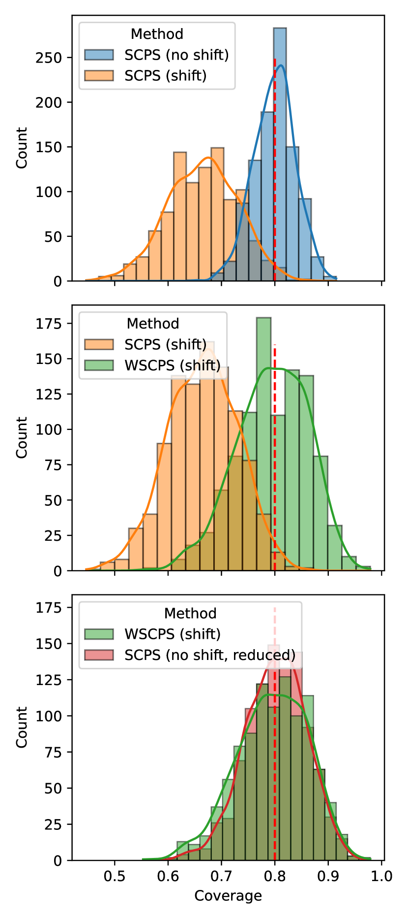
(a) Airfoil data

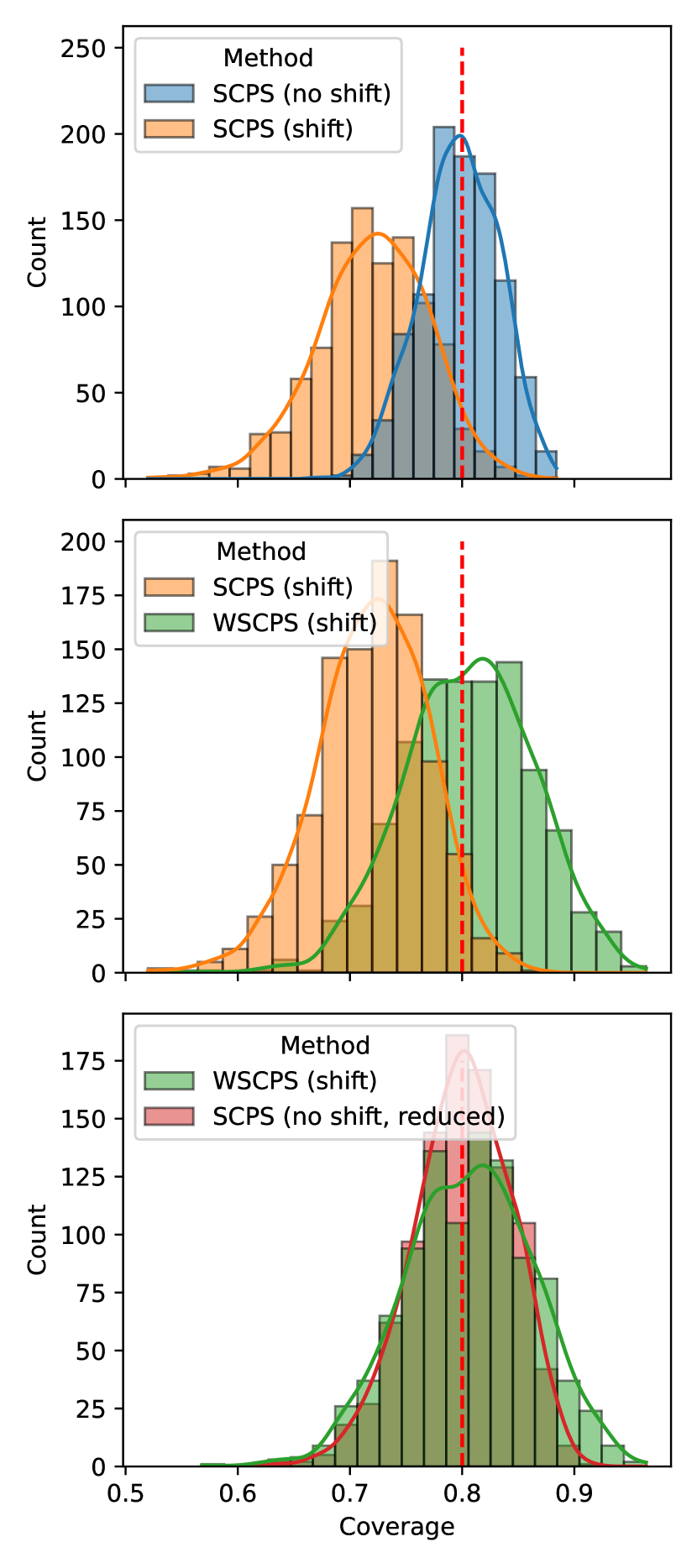
(b) Synthetic data

Figure 1: Empirical coverage of 80% prediction intervals from (W)SCPS, computed using 1000 different random splits of the airfoil and synthetic dataset.

Quality of predictive distribution under covariate shift

Figure 2 shows the performance of different SCPS in terms of CRPS across the different trials. We see a performance difference when a covariate shift is present and not. The WSCPS consistently (slightly) outperforms the SCPS under covariate shift for both datasets. However, it is difficult to see in the second row of Figure 2. Therefore, we also perform a post-hoc Friedman-Nemenyi test (see Figure 3). The SCPS under no shift with a calibration set size equal to the effective sample size of WSCPS has a significantly better CRPS score than WSCPS. This is expected since under covariate shift, the model $\hat{\mu}$ is trained on training data differently distributed as the test set, as Tibshirani et al. (2019) also indicated. Ideally, $\hat{\mu}$ should be adjusted for the covariate shift; however, we leave this for future work.

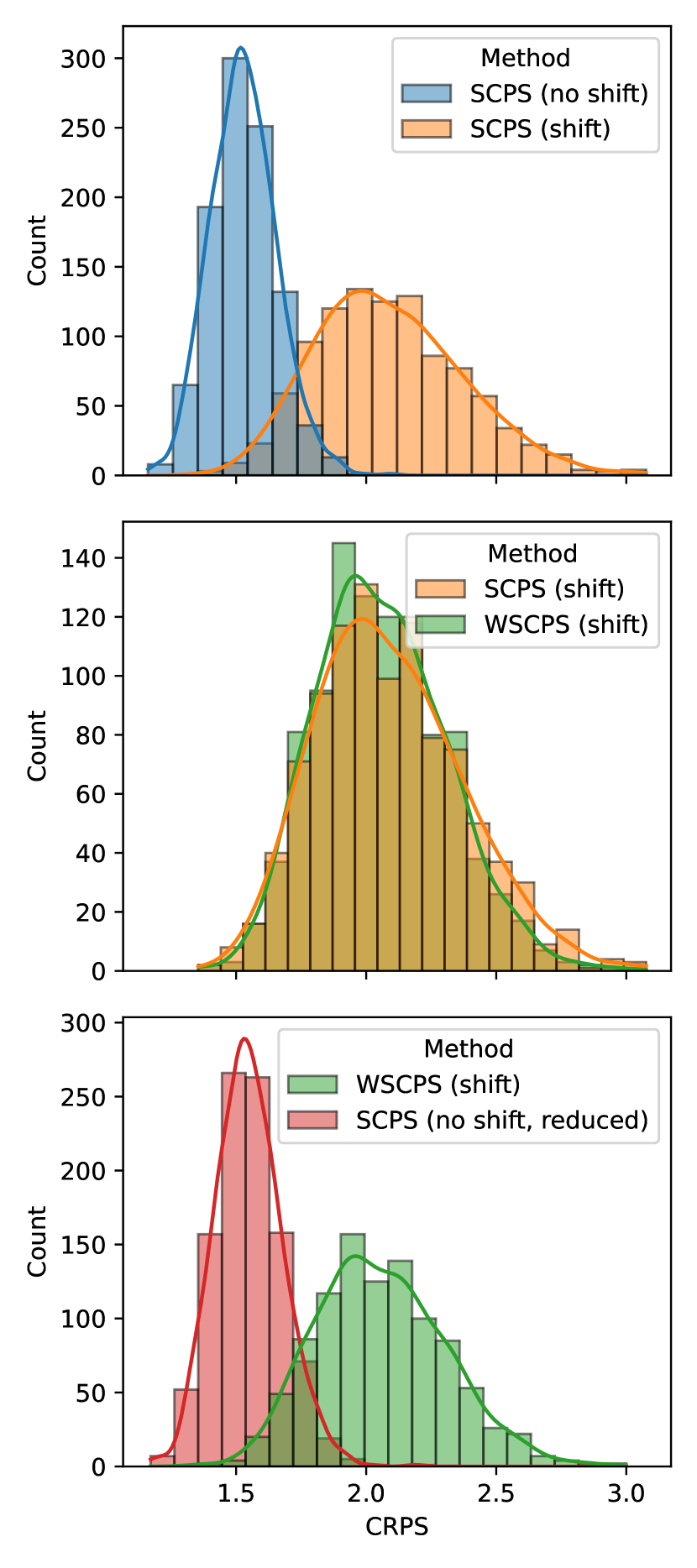
(a) Airfoil data

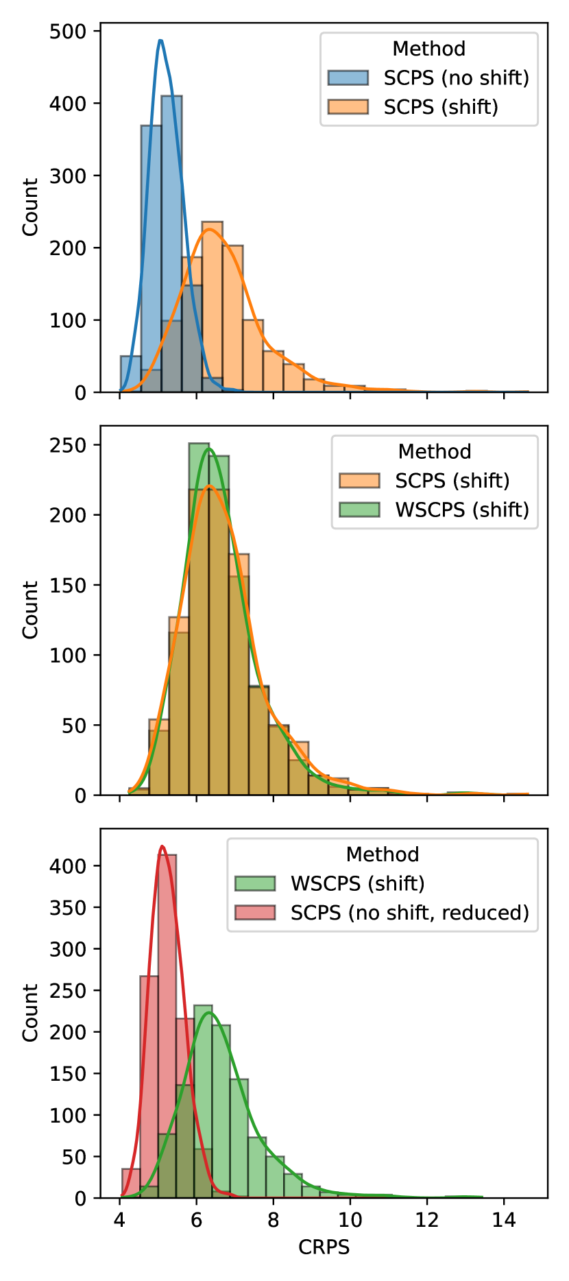
(b) Synthetic data

Figure 2: Empirical CRPS of (W)SCPS, computed using 1000 different experiment trials for both airfoil and synthetic datasets.

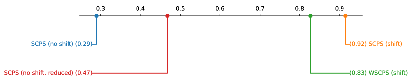
(a) Airfoil data

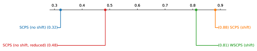
(b) Synthetic data

Figure 3: Post-hoc Friedman-Nemenyi test for CRPS.

Probabilistic calibration under covariate shift

We validate by simulation Conjecture 3, which states that under covariate shift, the weighted split conformal transducer produced $p$-values are distributed uniformly on $[0,1]$ when we know the likelihood ratio of the covariate distribution of the training and test set. The results of the simulation experiments, depicted in Figure 4, indicate that Conjecture 3 is empirically valid and that it breaks when we do not account for the covariate shift.

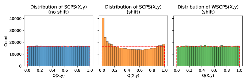
Figure 4: Distribution of p-values of SCPS under IID model (blue), covariate shift (orange), and WSCPS (green). The red dashed line represents the uniform distribution the p-values need to follow so that the (W)SCPS is probabilistically calibrated.

5 Conclusion

We have introduced a novel extension to Conformal Predictive Systems (CPS) to address covariate shifts in predictive modeling. Covariate shifts are a common challenge in real-world machine learning applications. Our proposed approach, Weighted (Split) Conformal Predictive Systems (W(S)CPS), leverages the likelihood ratio between training and testing data distributions to construct calibrated predictive distributions.

We outlined the theoretical framework of WCPS and WSCPS, demonstrating their formal definition and properties. Similarly, as Tibshirani et al. (2019), we built upon the foundation of CPS and extended the concept to handle covariate shifts effectively. Our theoretical analysis included conjectures regarding the probabilistic calibration of WCPS under covariate shift, paving the way for future research in this area. Additionally, we successfully validated these conjectures with simulation experiments.

In future work, we aim to provide rigorous proofs for the conjectures presented in this paper to establish the theoretical underpinnings of our proposed methods. Additionally, we will evaluate our proposed framework for counterfactual inference and incorporate it into our recently proposed Conformal Monte-Carlo meta-learners (Jonkers et al., 2024b), which opens the possibility of giving validity guarantees for predictive distributions of individual treatment effect beyond the randomized trial setting. Overall, our contributions offer a promising avenue for addressing covariate shifts in predictive modeling, with potential applications in diverse fields such as healthcare, finance, and climate science.

Appendix A Split Conformal Predictive System

For Split CPS (SCPS), the same procedure is followed as a split conformal prediction; the training sequence $z_{1:n}$ is split into two: a proper training sequence $z_{1:m}$ and calibration sequence $z_{m+1:n}$. Similarly as an CPS, an SCPS is defined as a function that is both a split conformal transducer (Definition 4) and an RPS (Definition 2) [Vovk et al., 2020a].

Definition 3 (Inductive (Split) Conformity Measure, Vovk et al. [2022]).

A split conformity measure is a measurable function $A:Z^{m}\times Z\rightarrow\mathbb{R}$ that is invariant with respect to permutations of the proper training sequence $z_{1:m}$.

Definition 4 (Split Conformal Transducer, Vovk et al. [2020a]).

The split conformal transducer determined by a split conformity measure $A$ (see Definition 3) is defined as,

$$\begin{split}Q(z_{1},...,z_{n},(x,y),\tau):=&\sum_{i=m+1}^{n}[R_{i}<R^{y}]\frac{1}{n-m+1}\\ &+\sum_{i=m+1}^{n}[R_{i}=R^{y}]\frac{\tau}{n-m+1}\\ &+\frac{\tau}{n-m+1}\end{split}$$ (19)

where conformity scores $R_{i}$ and $R^{y}$ are defined by

$$\begin{split}R_{i}&:=A(z_{1},...,z_{m},(x_{i},y_{i})),\qquad i=m+1,...,n,\\ R^{y}&:=A(z_{1},...,z_{m},(x,y)),\qquad y\in\mathbb{R}.\end{split}$$

Vovk et al. [2020a] proofs that any split conformal transducer is an RPS if and only if it is based on a balanced isotonic split conformity measure (Definition 6).

Definition 5 (Isotonic Split Conformity Measure, Vovk et al. [2020a]).

A split conformity measure $A$ is isotonic if, for all $m$, $z_{1:m}$, and $x$, $A(z_{1},...,z_{m},(x,y))$ is isotonic in $y$, i.e.,

$$y\leq y^{\prime}\Rightarrow A(z_{1},...,z_{m},(x,y))\leq A(z_{1},...,z_{m},(x,y^{\prime}))$$

Definition 6 (Balanced Isotonic Split Conformity Measure, Vovk et al. [2020a]).

An isotonic split conformity measure $A$ (see Definition 5) is balanced if, for any $m$ and $z_{1},...,z_{m}$, the set

$$\text{conv }A(z_{1},...,z_{m},(x,\mathbb{R})):=\text{conv }\{A(z_{1},...,z_{m},(x,y))|y\in\mathbb{R}\}$$

where conv stands for the convex closure in $\mathbb{R}$.

Appendix B Python Package: crepes-weighted

For the simulation experiments in this work, we implemented the proposed WSCPS and the WCP [Tibshirani et al., 2019] in crepes-weighted, which is an extension of crepes [Boström, 2022], a Python package that implements conformal classifiers, regressors, and predictive systems on top of any standard classifier and regressor. crepes-weighted relies on the same classes and functions as crepes, with the slight modification that for the ConformalRegressor and ConformalPredictiveSystem classes, the methods fit and predict needs to include the likelihood ratios of each calibration and test object respectively.

The source code of crepes-weighted is made open-source and can be found at https://github.com/predict-idlab/crepes-weighted.

References

- Vovk et al. [2019] Vladimir Vovk, Jieli Shen, Valery Manokhin, and Min-Ge Xie. Nonparametric predictive distributions based on conformal prediction. Machine Language, 108(3):445–474, March 2019. ISSN 0885-6125. doi:10.1007/s10994-018-5755-8. URL https://doi.org/10.1007/s10994-018-5755-8.
- Vovk et al. [2020a] Vladimir Vovk, Ivan Petej, Ilia Nouretdinov, Valery Manokhin, and Alexander Gammerman. Computationally efficient versions of conformal predictive distributions. Neurocomputing, 397:292–308, July 2020a. ISSN 0925-2312. doi:10.1016/j.neucom.2019.10.110. URL https://www.sciencedirect.com/science/article/pii/S0925231219316042.
- Vovk et al. [2018] Vladimir Vovk, Ilia Nouretdinov, Valery Manokhin, and Alex Gammerman. Conformal Predictive Distributions with Kernels. In Lev Rozonoer, Boris Mirkin, and Ilya Muchnik, editors, Braverman Readings in Machine Learning. Key Ideas from Inception to Current State: International Conference Commemorating the 40th Anniversary of Emmanuil Braverman’s Decease, Boston, MA, USA, April 28-30, 2017, Invited Talks, Lecture Notes in Computer Science, pages 103–121. Springer International Publishing, Cham, 2018. ISBN 978-3-319-99492-5. doi:10.1007/978-3-319-99492-5_4. URL https://doi.org/10.1007/978-3-319-99492-5_4.
- Vovk et al. [2020b] Vladimir Vovk, Ivan Petej, Paolo Toccaceli, Alexander Gammerman, Ernst Ahlberg, and Lars Carlsson. Conformal calibrators. In Proceedings of the Ninth Symposium on Conformal and Probabilistic Prediction and Applications, pages 84–99. PMLR, August 2020b. URL https://proceedings.mlr.press/v128/vovk20a.html. ISSN: 2640-3498.
- Boström et al. [2021] Henrik Boström, Ulf Johansson, and Tuwe Löfström. Mondrian conformal predictive distributions. In Proceedings of the Tenth Symposium on Conformal and Probabilistic Prediction and Applications, pages 24–38. PMLR, September 2021. URL https://proceedings.mlr.press/v152/bostrom21a.html.
- Johansson et al. [2023] Ulf Johansson, Tuwe Löfström, and Henrik Boström. Conformal Predictive Distribution Trees. Annals of Mathematics and Artificial Intelligence, June 2023. ISSN 1573-7470. doi:10.1007/s10472-023-09847-0. URL https://doi.org/10.1007/s10472-023-09847-0.
- Jonkers et al. [2024a] Jef Jonkers, Diego Nieves Avendano, Glenn Van Wallendael, and Sofie Van Hoecke. A novel day-ahead regional and probabilistic wind power forecasting framework using deep CNNs and conformalized regression forests. Applied Energy, 361:122900, May 2024a. ISSN 0306-2619. doi:10.1016/j.apenergy.2024.122900. URL https://www.sciencedirect.com/science/article/pii/S0306261924002836.
- Vovk [2022] Vladimir Vovk. Universal predictive systems. Pattern Recognition, 126:108536, June 2022. ISSN 0031-3203. doi:10.1016/j.patcog.2022.108536. URL https://www.sciencedirect.com/science/article/pii/S0031320322000176.
- Shafer and Vovk [2008] Glenn Shafer and Vladimir Vovk. A Tutorial on Conformal Prediction. Journal of Machine Learning Research, 9(12):371–421, 2008. ISSN 1533-7928. URL http://jmlr.org/papers/v9/shafer08a.html.
- Tibshirani et al. [2019] Ryan J Tibshirani, Rina Foygel Barber, Emmanuel Candes, and Aaditya Ramdas. Conformal Prediction Under Covariate Shift. In Advances in Neural Information Processing Systems, volume 32. Curran Associates, Inc., 2019. URL https://proceedings.neurips.cc/paper/2019/hash/8fb21ee7a2207526da55a679f0332de2-Abstract.html.
- Gibbs and Candes [2021] Isaac Gibbs and Emmanuel Candes. Adaptive Conformal Inference Under Distribution Shift. In Advances in Neural Information Processing Systems, volume 34, pages 1660–1672. Curran Associates, Inc., 2021. URL https://proceedings.neurips.cc/paper/2021/hash/0d441de75945e5acbc865406fc9a2559-Abstract.html.
- Prinster et al. [2022] Drew Prinster, Anqi Liu, and Suchi Saria. JAWS: Auditing Predictive Uncertainty Under Covariate Shift. Advances in Neural Information Processing Systems, 35:35907–35920, December 2022. URL https://proceedings.neurips.cc/paper_files/paper/2022/hash/e944bacecce6b06374ac39b260348db0-Abstract-Conference.html.
- Yang et al. [2022] Yachong Yang, Arun Kumar Kuchibhotla, and Eric Tchetgen Tchetgen. Doubly Robust Calibration of Prediction Sets under Covariate Shift, December 2022. URL http://arxiv.org/abs/2203.01761. arXiv:2203.01761 [math, stat].
- Gibbs and Candès [2023] Isaac Gibbs and Emmanuel Candès. Conformal Inference for Online Prediction with Arbitrary Distribution Shifts, October 2023. URL http://arxiv.org/abs/2208.08401. arXiv:2208.08401 [cs, stat].
- Jonkers et al. [2024b] Jef Jonkers, Jarne Verhaeghe, Glenn Van Wallendael, Luc Duchateau, and Sofie Van Hoecke. Conformal Monte Carlo Meta-learners for Predictive Inference of Individual Treatment Effects, February 2024b. URL http://arxiv.org/abs/2402.04906. arXiv:2402.04906 [cs, stat].
- Vovk et al. [2022] Vladimir Vovk, Alexander Gammerman, and Glenn Shafer. Algorithmic Learning in a Random World. Springer International Publishing, Cham, 2022. ISBN 978-3-031-06648-1 978-3-031-06649-8. doi:10.1007/978-3-031-06649-8. URL https://link.springer.com/10.1007/978-3-031-06649-8.
- Papadopoulos et al. [2002] Harris Papadopoulos, Kostas Proedrou, Volodya Vovk, and Alex Gammerman. Inductive Confidence Machines for Regression. In Tapio Elomaa, Heikki Mannila, and Hannu Toivonen, editors, Machine Learning: ECML 2002, Lecture Notes in Computer Science, pages 345–356, Berlin, Heidelberg, 2002. Springer. ISBN 978-3-540-36755-0. doi:10.1007/3-540-36755-1_29.
- Gretton et al. [2008] Arthur Gretton, Alex Smola, Jiayuan Huang, Marcel Schmittfull, Karsten Borgwardt, and Bernhard Schölkopf. Covariate Shift by Kernel Mean Matching. In Dataset Shift in Machine Learning. MIT Press, Cambridge, Mass., December 2008. ISBN 978-0-262-25510-3. URL https://direct.mit.edu/books/edited-volume/3841/chapter/125883/Covariate-Shift-by-Kernel-Mean-Matching.
- Reddi et al. [2015] Sashank Reddi, Barnabas Poczos, and Alex Smola. Doubly Robust Covariate Shift Correction. Proceedings of the AAAI Conference on Artificial Intelligence, 29(1), February 2015. ISSN 2374-3468. doi:10.1609/aaai.v29i1.9576. URL https://ojs.aaai.org/index.php/AAAI/article/view/9576.
- Boström [2022] Henrik Boström. crepes: a Python Package for Generating Conformal Regressors and Predictive Systems. In Proceedings of the Eleventh Symposium on Conformal and Probabilistic Prediction with Applications, pages 24–41. PMLR, August 2022. URL https://proceedings.mlr.press/v179/bostrom22a.html. ISSN: 2640-3498.
- Dua and Casey [2017] Dheeru Dua and Graff Casey. UCI machine learning repository. 2017.
- Kang and Schafer [2007] Joseph D. Y. Kang and Joseph L. Schafer. Demystifying Double Robustness: A Comparison of Alternative Strategies for Estimating a Population Mean from Incomplete Data. Statistical Science, 22(4):523–539, November 2007. ISSN 0883-4237, 2168-8745. doi:10.1214/07-STS227. URL https://projecteuclid.org/journals/statistical-science/volume-22/issue-4/Demystifying-Double-Robustness--A-Comparison-of-Alternative-Strategies-for/10.1214/07-STS227.full.
- Gneiting and Raftery [2007] Tilmann Gneiting and Adrian E Raftery. Strictly Proper Scoring Rules, Prediction, and Estimation. Journal of the American Statistical Association, 102(477):359–378, March 2007. ISSN 0162-1459. doi:10.1198/016214506000001437. URL https://doi.org/10.1198/016214506000001437. Publisher: Taylor & Francis _eprint: https://doi.org/10.1198/016214506000001437.
- Gneiting et al. [2007] Tilmann Gneiting, Fadoua Balabdaoui, and Adrian E. Raftery. Probabilistic forecasts, calibration and sharpness. Journal of the Royal Statistical Society: Series B (Statistical Methodology), 69(2):243–268, 2007. ISSN 1467-9868. doi:10.1111/j.1467-9868.2007.00587.x. URL https://onlinelibrary.wiley.com/doi/abs/10.1111/j.1467-9868.2007.00587.x.