: Attention-based pooling for interpretable image recognition

Abstract

Explanations obtained from transformer-based architectures in the form of raw attention, can be seen as a class-agnostic saliency map. Additionally, attention-based pooling serves as a form of masking the in feature space. Motivated by this observation, we design an attention-based pooling mechanism intended to replace Global Average Pooling (gap) at inference. This mechanism, called Cross-Attention Stream (), comprises a stream of cross attention blocks interacting with features at different network depths. enhances interpretability in models, while preserving recognition performance.

1 Introduction

Convolutional neural networks (CNN) have attained tremendous success in computer vision [22, 30], but interpreting their predictions remains challenging. Most explanations are based on saliency maps, using methods derived from class activation mapping (CAM). Vision transformers [13] are now strong competitors of convolutional networks, characterized by global interactions between patch embeddings in the form of self attention. Based on the classification (cls) token, an explanation map in the form of raw attention can be constructed. However, these maps are class-agnostic, often of low quality [6], and dedicated interpretability methods are required to explain models [9].

In CNNs, features are pooled into a global representation by global average pooling (GAP). In transformers, a global representation is obtained by cross-attention between patch embeddings and the cls token. In this work, we make a connection between CAM-based saliency maps and raw attention from the cls token, observing that attention-based pooling is a form of masking in the feature space. Motivated by this observation, we design a pooling mechanism that generates a global representation to be used at inference, replacing GAP and improving interpretability.

Our approach, called Cross-Attention Stream (), consists of a branch in parallel with the backbone network, allowing interactions between feature maps and the cls token through cross-attention at different stages of the network. The cls token embedding is a learnable parameter and, at the output of the stream, provides a global image representation for classification.

More specifically, we make the following contributions:

1. We demonstrate that attention-based pooling in vision transformers is the same as soft masking by a class-agnostic CAM-based saliency map (subsection 3.2).

2. We design an attention-based pooling mechanism, inject it in convolutional networks to replace GAP and study its effect on post-hoc interpretability (subsection 3.3).

3. We show improved explanations for a trained model and provides a class-agnostic raw attention map (section 4).

Figure 1: Cross-Attention Stream (Cross-Attention Stream () applied to ResNet-based architectures. Given a network $f$, we replace global average pooling (gap) by a learned, attention-based pooling mechanism implemented as a stream in parallel to $f$. The feature tensor $F_{\ell}\in^{p_{\ell}\times d_{\ell}}$ (key) obtained by stage Res-$\ell$ of $f$ interacts with a cls token (query) embedding $\mathbf{q}_{\ell}\in^{d_{\ell}}$ in block CA-$\ell$, which contains cross attention (6) followed by a linear projection (10) to adapt to the dimension of $F_{\ell+1}$. Here, $p_{\ell}$ is the number of patches (spatial resolution) and $d_{\ell}$ the embedding dimension. The query is initialized by a learnable parameter $\mathbf{q}_{0}\in^{d_{0}}$, while the output $\mathbf{q}_{5}$ of the last cross attention block is used as a global image representation into the classifier.

2 Related work

Deep neural networks interpretability is investigated though Post-hoc interpretability or Transparency  [28, 20, 55].

Post-hoc interpretability

considers the model as a black-box and provides explanations based on input and output observations. These methods can be grouped into sets of possibly overlapping categories. Gradient-based methods [1, 45, 3, 43, 44, 2, 46] use gradient information to visualize the contribution of different input regions in an image. CAM-based methods [49, 8, 41, 16, 25, 12] compute saliency maps as a linear combination of feature maps to highlight salient regions in the input image. Occlusion or masking-based methods [32, 15, 14, 40, 37] instead compute saliency maps based on the prediction changes induced by masking the input image. Finally, learning-based methods [7, 10, 33, 60, 40] learn additional models or branches to produce explanations for a given input.

Transparency

modifies the model or its training process to explain it. These approaches are grouped according to the nature of the explanation they provide. Rule-based methods  [50, 51] approximate the model using a decision tree as a proxy. Hidden semantic-methods  [4, 58, 54, 56] learn disentangled semantics following a hierarchical structure or object-level concepts. Prototype-based methods learn prototypes seen in training images to explain models from intermediate representations. Attribution-based methods [24, 59, 39, 17] propose modifications to the network or its training process, improving interpretable properties of post-hoc attribution methods. Finally, saliency-guided training  [24, 26] design and train a model that aligns images with their saliency based masks during training enhancing recognition and interpretability properties.

Our approach aligns with attribution-based methods. Specifically, we introduce a learnable cross-attention stream, producing a representation that replaces gap.

Attention-based architectures

Attention is a mechanism introduced into convolutional neural networks to enhance their recognition capabilities  [5, 36, 42]. Following the success of vision transformers (ViT)  [13], fully attention-based architectures are now competitive with convolutional neural networks, while drawing inspiration from them to enhance their recognition capabilities  [19, 52, 29, 23].

Unlike similar approaches combining ideas from convolutions in transformers [31, 27, 47], we propose to add an attention-based pooling mechanism in convolutional models, enhancing post-hoc interpretability properties without degrading classification accuracy.

3 Method

	Input image	Raw Attention	Grad-CAM		Grad-CAM++		Score-CAM
			GAP		GAP		GAP
CRT screen
Snowboard

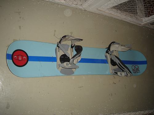
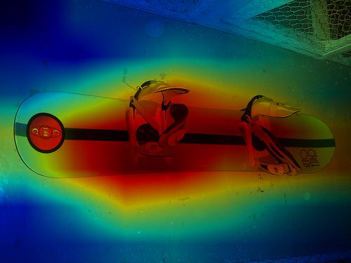
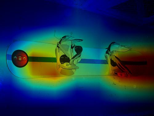
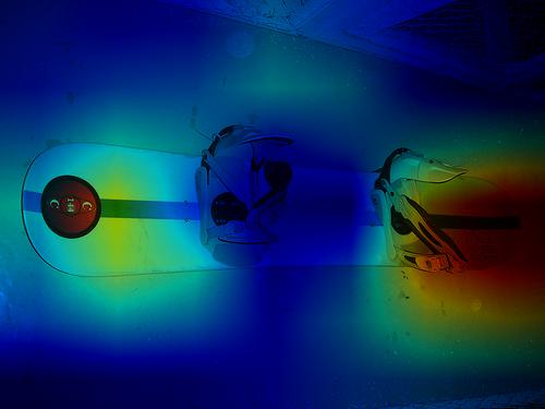
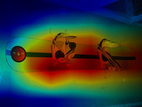
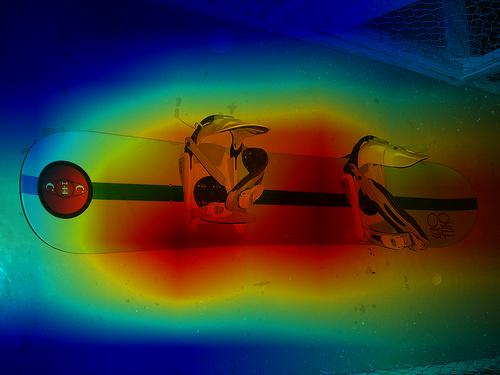
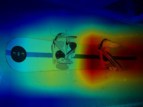
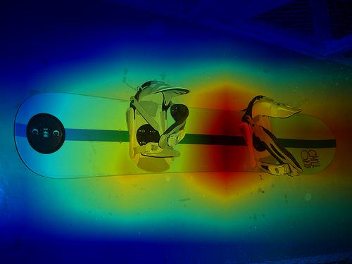
Figure 2: Comparison of saliency maps generated by different CAM-based methods, using GAP and our , on ImageNet images. The raw attention is the one used for pooling by .

3.1 Preliminaries and background

Notation

Let $f:\mathcal{X}\rightarrow^{C}$ be a classifier network that maps an input image $\mathbf{x}\in\mathcal{X}$ to a logit vector $\mathbf{y}=f(\mathbf{x})\in^{C}$, where $\mathcal{X}$ is the image space and $C$ is the number of classes. A class probability vector is obtained by $\mathbf{p}=\operatorname{softmax}(\mathbf{y})$. The logit and probability of class $c$ are respectively denoted by $y^{c}$ and $p^{c}=\operatorname{softmax}(\mathbf{y})^{c}$. Let $\mathbf{F}_{\ell}\in^{w_{\ell}\times h_{\ell}\times d_{\ell}}$ be the feature tensor at layer $\ell$ of the network, where $w_{\ell}\times h_{\ell}$ is the spatial resolution and $d_{\ell}$ the embedding dimension, or number of channels. The feature map of channel $k$ is denoted by $F^{k}_{\ell}\in^{w_{\ell}\times h_{\ell}}$.

CAM-based saliency maps

Given a class of interest $c$ and a layer $\ell$, we consider the saliency maps $S^{c}_{\ell}\in^{w_{\ell}\times h_{\ell}}$ given by the general formula

$$S^{c}_{\ell}\mathrel{:=}h\left(\sum_{k}\alpha^{c}_{k}F^{k}_{\ell}\right),$$ (1)

where $\alpha^{c}_{k}$ are weights defining a linear combination over channels and $h$ is an activation function. Assuming global average pooling (GAP) of the last feature tensor $\mathbf{F}_{L}$ followed by a linear classifier, CAM [57] is defined for the last layer $L$ only, with $h$ being the identity mapping and $\alpha^{c}_{k}$ the classifier weight connecting channel $k$ with class $c$.

Self-attention

Let $X_{\ell}\in^{t_{\ell}\times d_{\ell}}$ denote the sequence of token embeddings of a vision transformer [13] at layer $\ell$, where $t_{\ell}\mathrel{:=}w_{\ell}h_{\ell}+1$ is the number of tokens, including patch tokens and the cls token, and $d_{\ell}$ is the embedding dimension. The attention matrix $A\in^{t_{\ell}\times t_{\ell}}$ expresses pairwise dot-product similarities between queries ($Q$) and keys ($K$), normalized by softmax over rows:

$$A=\operatorname{softmax}\left(\frac{QK^{\top}}{\sqrt{d_{\ell}}}\right).$$ (2)

For each token, the self-attention operation is then defined as an average of all values ($V$) weighted by attention $A$:

$${\textsc{sa}}(X_{\ell})\mathrel{:=}AV\in^{t_{\ell}\times d_{\ell}}.$$ (3)

At the last layer $L$, the cls token embedding is used as a global representation for classification as it gathers information from all patches by weighted averaging, replacing gap. Thus, at the last layer, it is only cross-attention between cls and the patch tokens that matters.

3.2 Motivation

Cross-attention

Let matrix $F_{\ell}\in^{p_{\ell}\times d_{\ell}}$ be a reshaping of feature tensor $\mathbf{F}_{\ell}$ at layer $\ell$, where $p_{\ell}\mathrel{:=}w_{\ell}h_{\ell}$ is the number of patch tokens without cls, and let $\mathbf{q}_{\ell}\in^{d_{\ell}}$ be the cls token embedding at layer $\ell$. By focusing on the cross-attention only between the cls (query) token $\mathbf{q}_{\ell}$ and the patch (key) tokens $F_{\ell}$, attention $A$ (2) is now a $1\times p_{\ell}$ matrix that can be written as a vector $\mathbf{a}\in^{p_{\ell}}$

$$\mathbf{a}=A^{\top}=\operatorname{softmax}\left(\frac{F_{\ell}\mathbf{q}_{\ell}}{\sqrt{d_{\ell}}}\right).$$ (4)

Here, $F_{\ell}\mathbf{q}_{\ell}$ expresses the pairwise similarities between the global cls feature $\mathbf{q}_{\ell}$ and the local patch features $F_{\ell}$. Now, by replacing $\mathbf{q}_{\ell}$ by an arbitrary vector ${\boldsymbol{\alpha}}\in^{d_{\ell}}$ and writing the feature matrix as $F_{\ell}=(\mathbf{f}_{\ell}^{1}\dots\mathbf{f}_{\ell}^{d_{\ell}})$, attention (4) becomes

$$\mathbf{a}=h_{\ell}(F_{\ell}{\boldsymbol{\alpha}})=h_{\ell}\left(\sum_{k}\alpha_{k}\mathbf{f}_{\ell}^{k}\right).$$ (5)

This takes the same form as (1), with feature maps $F_{\ell}^{k}$ vectorized as $\mathbf{f}_{\ell}^{k}$ and the activation function defined as $h_{\ell}(\mathbf{x})=\operatorname{softmax}(\mathbf{x}/\sqrt{d_{\ell}})$. We thus observe the following.

Pairwise similarities between one query and all patch token embeddings in cross-attention are the same as a linear combination of feature maps in CAM-based saliency maps.

One difference between (1) and (5) is that (5) is class-agnostic, although it could be extended by using one query vector per class. For simplicity, we choose the class-agnostic form. We also choose to have no query/key projections. However, we do provide additional experiments in the appendix.

Pooling or masking

We integrate an attention mechanism into a network such that making a prediction and explaining it are inherently connected. In particular, considering cross-attention only between cls and patch tokens (4), equation (3) becomes

$${\textsc{ca}}_{\ell}(\mathbf{q}_{\ell},F_{\ell})\mathrel{:=}F_{\ell}^{\top}\mathbf{a}=F_{\ell}^{\top}h_{\ell}(F_{\ell}\mathbf{q}_{\ell})\in^{d_{\ell}}.$$ (6)

By writing the transpose of feature matrix as $F_{\ell}^{\top}=({\boldsymbol{\phi}}_{\ell}^{1}\dots\boldsymbol{\phi}_{\ell}^{p_{\ell}})$ where ${\boldsymbol{\phi}}_{\ell}^{i}\in^{d_{\ell}}$ is the feature of patch $i$, this is a weighted average of the local patch features $F_{\ell}^{\top}$ with attention vector $\mathbf{a}=(a_{1},\dots,a_{p_{\ell}})$ expressing the weights:

$${\textsc{ca}}_{\ell}(\mathbf{q}_{\ell},F_{\ell})\mathrel{:=}F_{\ell}^{\top}\mathbf{a}=\sum_{i}a_{i}{\boldsymbol{\phi}}_{\ell}^{i}.$$ (7)

We can think of it as as feature reweighting or soft masking in the feature space, followed by gap.

Now, considering that $\mathbf{a}$ is obtained exactly as CAM-based saliency maps (5), this operation is similar to occlusion (masking)-based methods [32, 15, 14, 40, 37, 49, 53] and evaluation metrics [8, 32], where a CAM-based saliency map is commonly used to mask the input image. We thus observe the following.

Attention-based pooling is a form of feature reweighting or soft masking in the feature space followed by gap, where the weights are given by a class-agnostic CAM-based saliency map.

3.3 Cross-attention stream

Motivated by these observations, we design a Cross-Attention Stream () in parallel to any network. It takes input features at key locations of the network and uses cross-attention to build a global image representation and replace gap before the classifier. An example is shown in Figure 1, applied to a ResNet-based architecture.

Architecture

More formally, given a network $f$, we consider points between blocks of $f$ where critical operations take place, such as change of spatial resolution or embedding dimension, e.g. between residual blocks on ResNet. We decompose $f$ at these points as

$$f=g\circ{\textsc{gap}}\circ f_{L}\circ\dots\circ f_{0}$$ (8)

such that features $F_{\ell}\in^{p_{\ell}\times d_{\ell}}$ of layer $\ell$ are initialized as $F_{-1}=\mathbf{x}$ and updated according to

$$F_{\ell}=f_{\ell}(F_{\ell-1})$$ (9)

for $0\leq\ell\leq L$, where $p_{\ell}$ is the number of patch tokens and $d_{\ell}$ the embedding dimension of stage $\ell$. The last layer features $F_{L}$ are followed by gap and $g:^{d_{L}}\to^{C}$ is the classifier, mapping to the logit vector $\mathbf{y}$.

In parallel, we initialize a classification token embedding as a learnable parameter $\mathbf{q}_{0}\in^{d_{0}}$ and we build a sequence of updated embeddings $\mathbf{q}_{\ell}\in^{d_{\ell}}$ along a stream that interacts with $F_{\ell}$ at each stage $\ell$. Referring to the global representation $\mathbf{q}_{\ell}$ as query or cls and to the local image features $F_{\ell}$ as key or patch embeddings, the interaction consists of cross-attention followed by a linear projection $W_{\ell}\in^{d_{\ell+1}\times d_{\ell}}$ to account for changes of embedding dimension between the corresponding stages of $f$:

$$\mathbf{q}_{\ell+1}=W_{\ell}\cdot{\textsc{ca}}_{\ell}(\mathbf{q}_{\ell},F_{\ell}),$$ (10)

for $0\leq\ell\leq L$, where ${\textsc{ca}}_{\ell}$ is defined as in (6).

Image features do not change by injecting our into network $f$. However, the final global image representation does, hence the prediction does too. In particular, at the last stage $L$, $\mathbf{q}_{L+1}$ is used as a global image representation for classification, replacing gap over $F_{L}$. Therefore, final prediction is $g(\mathbf{q}_{L+1})\in^{C}$. Unlike gap, the weights of different image patches in the linear combination are non-uniform, enhancing the contribution of relevant patches in the prediction.

Training

The network $f$ is pretrained and remains frozen while we learn the parameters of our on the same training set as $f$. The classifier is kept frozen too. Referring to (8), $f_{0},\dots,f_{L}$ and $g$ are fixed, while gap is replaced by learned weighted averaging, with the weights obtained by the .

Inference

As it stands, the is an addition to the baseline architecture, which enhances the interpretability properties of a model. We thus investigate interpretability using CAM-based methods on both baseline gap and in the following section.

4 Experiments

Experimental setup

We train and evaluate our models on the ImageNet ILSVRC-2012 dataset [11], using the training and validation sets respectively. We experiment on pretrained and frozen ResNets [22] and ConvNeXt [30] models and provide more details in the appendix. We measure the interpretability properties of our approach by first generating saliency maps employing existing methods based on CAM (Grad-CAM [41], Grad-CAM++ [8], ScoreCAM [49]) with and without . Then, following [53], we compute changes in the predictive power of a masked image measured by average drop (AD) [8] and average gain (AG) [53], the proportion of better explanations measured by average increase (AI) [8] and finally the impact of different extents of masking via insertion (I) and deletion (D) [32].

Qualitative results

In Figure 2, we show saliency maps obtained using either gap and ca, as well as the raw attention representation from . We observe that CAM-based attributions obtained using our ca are similar to those generated with gap. We expect this behaviour as we do not modify the model or the weighting coefficients. Since raw attention is class-agnostic, it can be used to gain insight on what the model attends to in unseen data. We iterate upon this in the appendix.

Quantitative evaluation

Network	Pooling					Acc$\uparrow$
ResNet-50	gap					74.55
	ca					74.70
ConvNeXt-B	gap					83.72
	ca					83.51
Network	Attribution	Pooling	AD$\downarrow$	AG$\uparrow$	AI$\uparrow$	I$\uparrow$	D$\downarrow$
ResNet-50	Grad-CAM	gap	13.04	17.56	44.47	72.57	13.24
		ca	12.54	22.67	48.56	75.53	13.50
	Grad-CAM++	gap	13.79	15.87	42.08	72.32	13.33
		ca	13.99	19.29	44.60	75.21	13.78
	Score-CAM	gap	8.83	17.97	48.46	71.99	14.31
		ca	7.09	23.65	54.20	74.91	14.68
ConvNeXt-B	Grad-CAM	gap	33.72	2.43	15.25	52.85	29.57
		ca	19.45	13.96	32.89	86.38	45.29
	Grad-CAM++	gap	34.01	2.37	15.60	52.83	29.17
		ca	36.69	8.00	21.95	85.39	53.42
	Score-CAM	gap	43.55	2.23	15.67	50.96	39.49
		ca	23.51	11.04	27.35	83.41	60.53

Table 1: Interpretability metrics of vs. baseline gap for different networks and interpretability methods on ImageNet.

In Table 1, we compare the interpretability properties when using our ca vs. gap. In the appendix we provide comparisons with more models and datasets. We observe that provides consistent improvements over gap in terms of AD, AG, AI and I metrics, while performing lower on D. Deletion (D) has raised concerns in previous works [9, 53]. As (D) gradually blackens pixels, out-of-distribution data [18, 21, 34] is produced, possibly introducing bias [38]. Moreover, non-spread attributions tend to perform better [53], which is likely the reason for lower performance.

5 Conclusion

In this work we observe that attention-based pooling in transformers is similar if not the same as forming a class agnostic CAM-based attribution. Based on this observation, we build upon this representation to mask features prior to the classification layers of a model, enhancing interpretability of existing image recognition models using gap. Our method improves interpretability metrics while maintaining recognition performance.

6 Acknowledgement

This work has received funding from the UnLIR ANR project (ANR-19-CE23-0009), the Excellence Initiative of Aix-Marseille Universite - A*Midex, a French “Investissements d’Avenir programme” (AMX-21-IET-017). Part of this work was performed using HPC resources from GENCI-IDRIS (Grant 2020-AD011011853 and 2020-AD011013110)

Appendix A More on the connection between Attention and CAM

Following the explanation of Cross-Attention acting as a class agnostic version of CAM demonstrated in subsection 3.2, we provide a visual explanation of this connection in Figure 3.

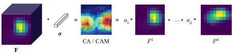
Figure 3: Visualization of eq. (5). On the left, a feature tensor $\mathbf{F}\in^{w\times h\times d}$ is multiplied by the vector ${\boldsymbol{\alpha}}\in^{d}$ in the channel dimension, like in $1\times 1$ convolution, where $w\times h$ is the spatial resolution and $d$ is the number of channels. This is cross attention (CA) [13] between the query ${\boldsymbol{\alpha}}$ and the key $\mathbf{F}$. On the right, a linear combination of feature maps $F^{1},\dots,F^{d}\in^{w\times h}$ is taken with weights $\alpha_{1},\dots,\alpha_{d}$. This is a class activation mapping (CAM) [57] with class agnostic weights. Eq. (5) expresses the fact that these two quantities are the same, provided that ${\boldsymbol{\alpha}}=(\alpha_{1},\dots,\alpha_{d})$ and $\mathbf{F}$ is reshaped as $F=(\mathbf{f}^{1}\dots\mathbf{f}^{d})\in^{p\times d}$, where $p=wh$ and $\mathbf{f}^{k}=\operatorname{vec}(F^{k})\in^{p}$ is the vectorized feature map of channel $k$.

Appendix B More on experimental setup

Implementation details

Following the training recipes from the pytorch models, we choose the ResNet protocol given its simplicity. Thus, we train over 90 epochs with SGD optimizer with momentum 0.9 and weight decay $10^{-4}$. We start our training with a learning rate of 0.1 and decrease it every 30 epochs by a factor of 10. Our models are trained on 8 V100 GPUs with a batch size 32 per GPU, thus global batch size 256. We follow the same protocol for both ResNet and ConvNeXt, though a different protocol might lead to improvements on ConvNeXt.

Appendix C More Visualizations

Corridor		Greenhouse		Pool Inside		Wine Cellar
Input image	Raw Attention	Input image	Raw Attention	Input image	Raw Attention	Input image	Raw Attention

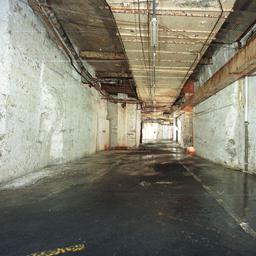
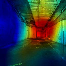
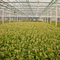
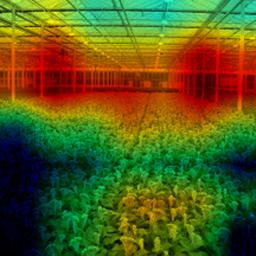
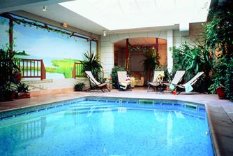
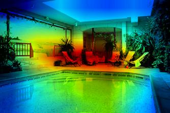
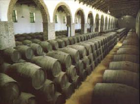
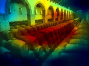
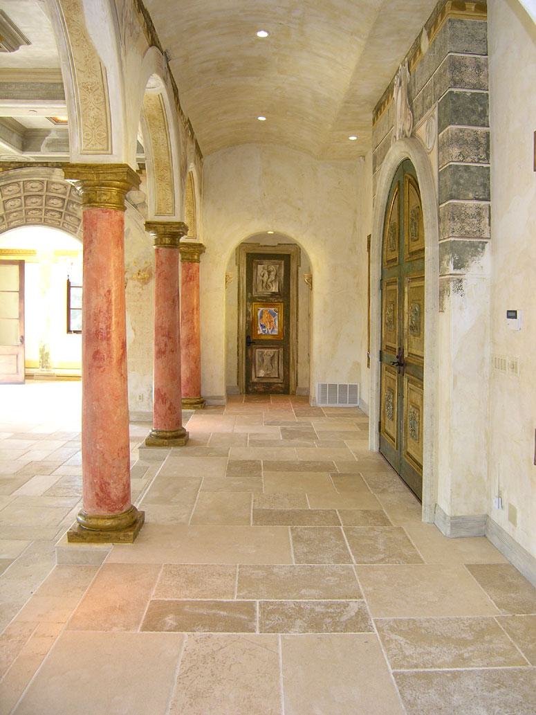
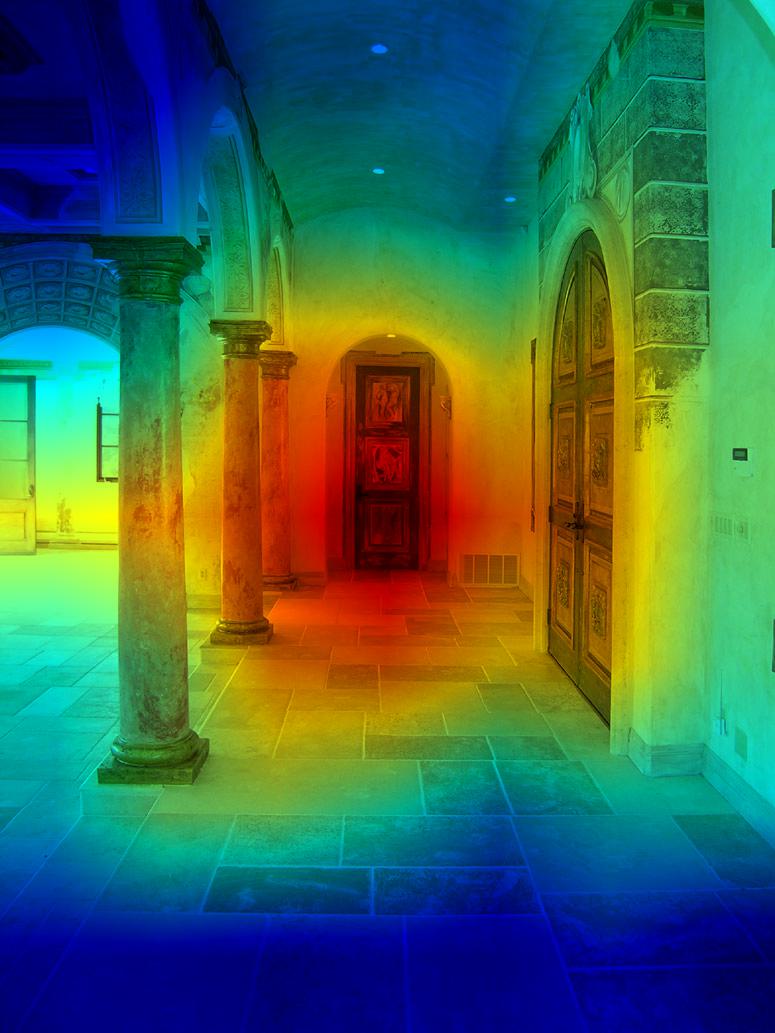
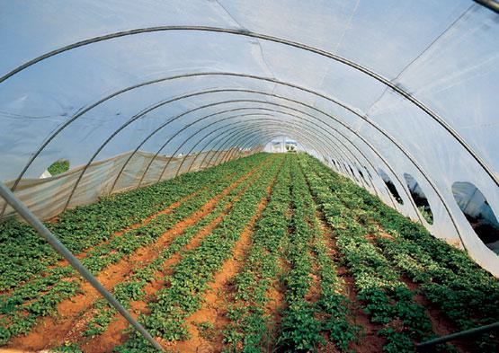
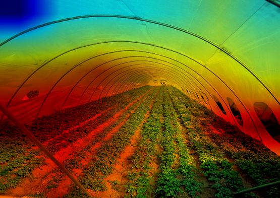
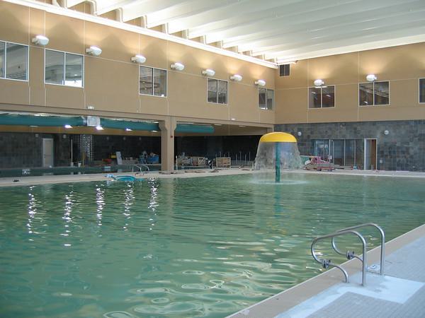
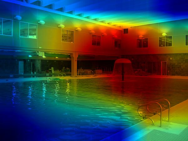
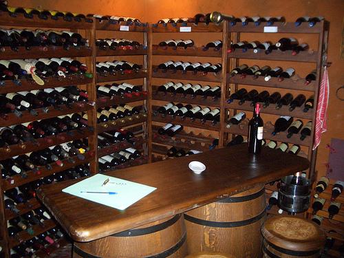
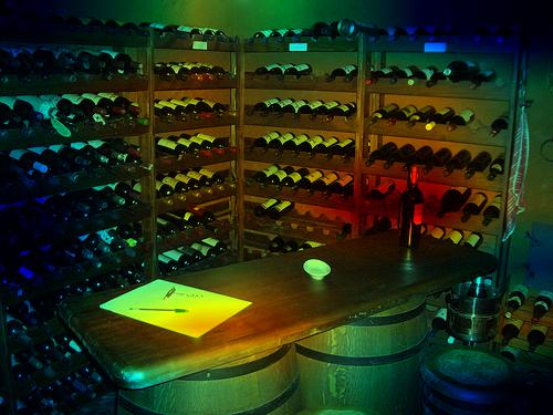
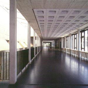
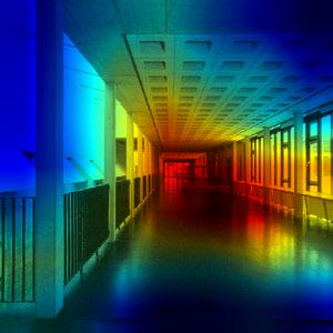
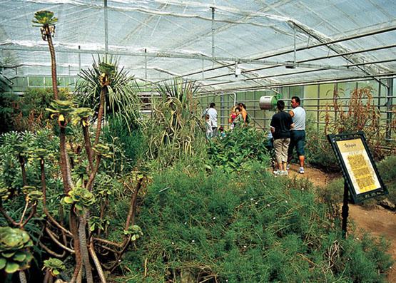
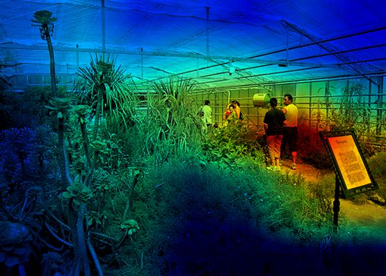
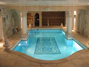
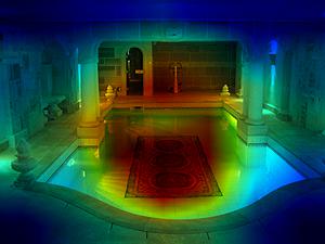
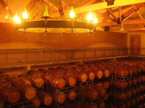
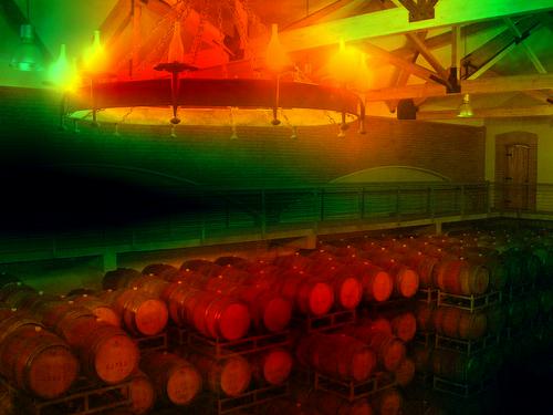
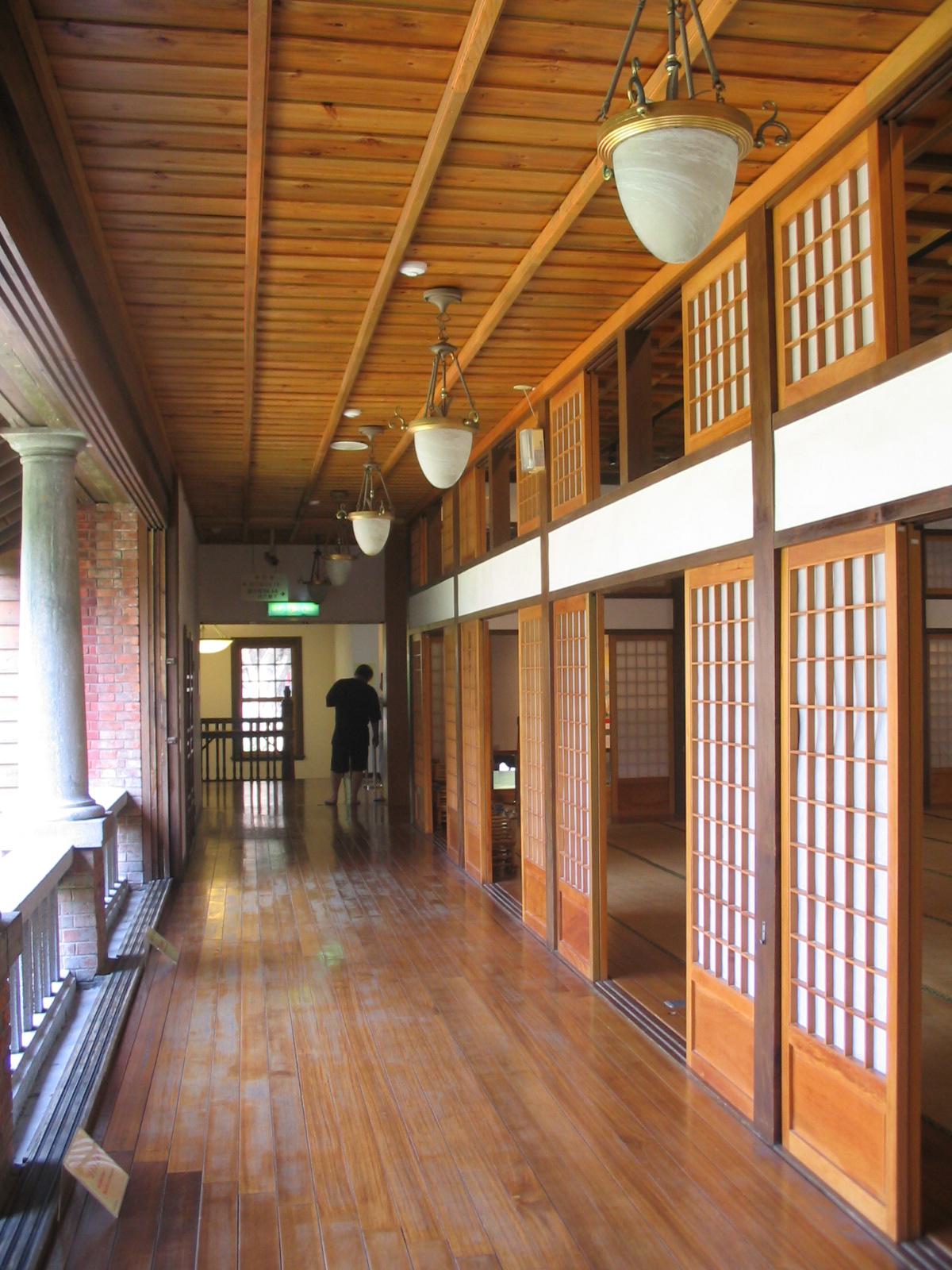
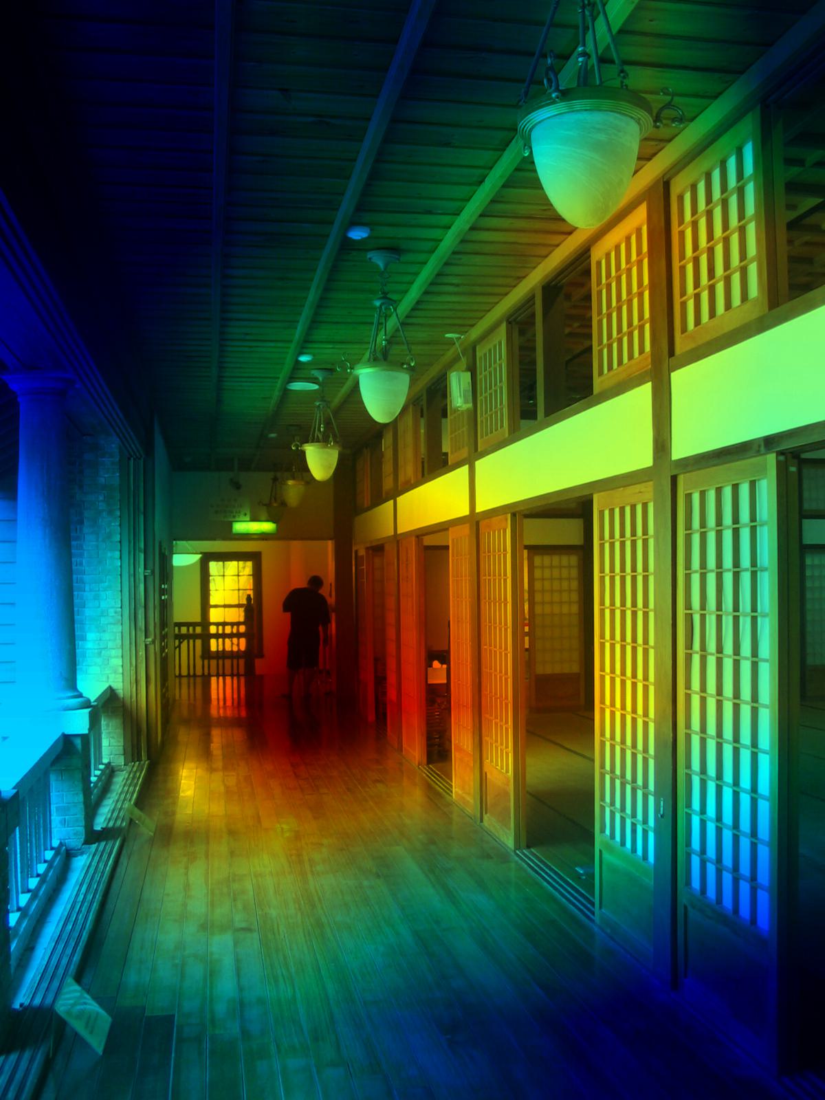
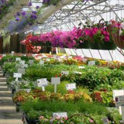
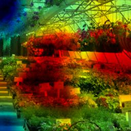
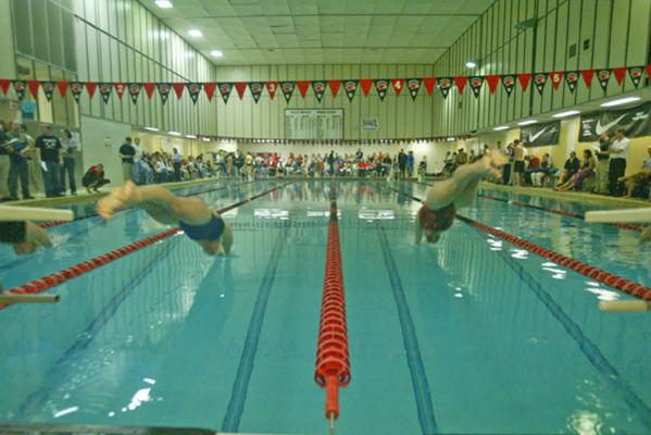
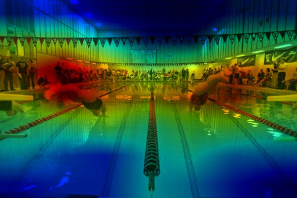
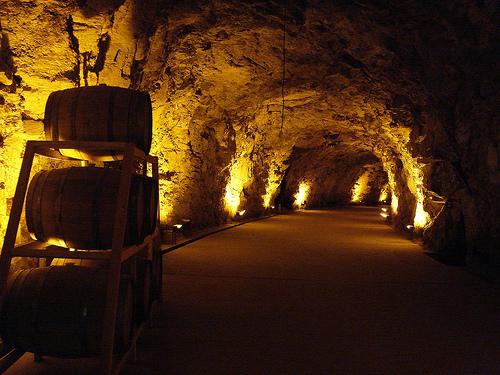
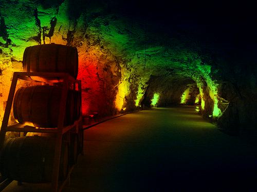
Figure 4: Raw attention maps obtained from our on images of the MIT 67 Scenes dataset [35] on classes that do not exist in ImageNet. The network sees them at inference for the first time.

In addition, Figure 4 shows examples of images from the MIT 67 Scenes dataset [35] along with raw attention maps obtained by . These images come from four classes that do not exist in ImageNet and the network sees them at inference for the first time. Nevertheless, the attention maps focus on objects of interest in general.

Appendix D More Architectures

Table Table 2 presents interpretability metrics for both ResNet18 and ConvNeXt-S. Complementary experiments are reported on Table 3 for CUB and Pascal VOC for ResNet 50.

Network	Attribution	Pooling	AD$\downarrow$	AG$\uparrow$	AI$\uparrow$	I$\uparrow$	D$\downarrow$
ResNet-18	Grad-CAM	gap	17.64	12.73	41.21	63.13	10.66
		ca	16.99	17.22	44.95	65.94	10.68
	Grad-CAM++	gap	19.05	11.16	37.99	62.80	10.75
		ca	19.02	14.76	40.82	65.53	10.82
	Score-CAM	gap	13.64	12.98	44.53	62.56	11.37
		ca	11.53	18.12	50.32	65.33	11.51
ConvNeXt-S	Grad-CAM	gap	42.99	1.69	12.60	48.42	30.12
		ca	22.09	14.91	32.65	84.82	43.02
	Grad-CAM++	gap	56.42	1.32	10.35	48.28	33.41
		ca	51.87	9.40	20.55	84.28	52.58
	Score-CAM	gap	74.79	1.29	10.10	47.40	38.21
		ca	64.21	8.81	18.96	82.92	57.46

Table 2: of vs. baseline gap for more networks and interpretability methods on ImageNet.

CUB-200-2011 - ResNet-50
	Pooling					Acc$\uparrow$
	gap					76.96
	ca					75.90
Interpretability Metrics
Method	Pooling	AD$\downarrow$	AG$\uparrow$	AI$\uparrow$	I$\uparrow$	D$\downarrow$
Grad-CAM	gap	10.87	10.29	45.81	65.71	6.17
	ca	10.44	17.61	53.54	74.60	6.56
Grad-CAM++	gap	11.35	9.68	44.32	65.64	5.92
	ca	11.01	16.50	51.63	74.64	6.21
Score-CAM	gap	9.05	10.62	48.90	65.58	5.94
	ca	6.37	19.50	60.41	74.22	2.14
Pascal VOC 2012 - ResNet-50
	Pooling					mAP$\uparrow$
	gap					78.32
	ca					78.35
Interpretability Metrics
Method	Pooling	AD$\downarrow$	AG$\uparrow$	AI$\uparrow$	I$\uparrow$	D$\downarrow$
Grad-CAM	gap	12.61	9.68	27.88	89.10	59.39
	ca	12.77	15.46	34.53	88.53	59.16
Grad-CAM++	gap	12.25	9.68	27.62	89.34	54.23
	ca	12.28	16.76	34.87	89.02	53.34
Score-CAM	gap	14.8	6.76	36.41	71.10	39.95
	ca	10.96	21.35	43.82	89.21	51.44

Table 3: Accuracy, respectively mean Average Precision, and interpretability metrics of vs. baseline gap for ResNet-50 on CUB and Pascal dataset.

Results on CUB in Table 3 show that our consistently provides improvements when the model is fine-tuned on a smaller fine-grained dataset.

Appendix E Ablation Experiments

We conduct ablation experiments on ResNet50 because of its modularity and ease of modification. We investigate the effect of the cross attention block design, the placement of the relative to the backbone network.

Cross attention block design

Following transformers [48, 13], it is possible to add more layers in the cross attention block. We consider a variant referred to as proj$\to$ca, which uses linear projections $W_{\ell}^{K},W_{\ell}^{V}\in^{d_{\ell}\times d_{\ell}}$ on the key and value

$${\textsc{ca}}_{\ell}(\mathbf{q}_{\ell},F_{\ell})\mathrel{:=}(F_{\ell}W^{V}_{\ell})^{\top}h_{\ell}(F_{\ell}W^{K}_{\ell}\mathbf{q}_{\ell})\in^{d_{\ell}},$$ (11)

while  (10) remains.

Block Type	$\#$Params	Accuracy
ca	6.96M	74.70
proj$\to$ca	18.13M	74.41

Table 4: Different cross attention block design for . Classification accuracy and parameters using ResNet-50 on ImageNet. $\#$Param: parameters of only.

Results are reported in Table 4. We observe that the stream made of vanilla CA blocks  (6) offers slightly better accuracy than projections, while having less parameters. We also note that most of the computation takes place in the last residual stages, where the channel dimension is the largest. To keep our design simple, we choose the vanilla solution without projections  (6) by default.

placement

To validate the design of , we measure the effect of its depth on its performance vs. the baseline gap in terms of both classification accuracy / number of parameters and classification metrics for interpretability. In particular, we place the stream in parallel to the network $f$, starting at stage $\ell$ and running through stage $L$, the last stage of $f$, where $0\leq\ell\leq L$. Results are reported in Table 5.

Accuracy and Parameters
	Placement	CLS dim		#Param		Acc$\uparrow$
	$S_{0}-S_{4}$	$64$		6.96M		74.70
	$S_{1}-S_{4}$	$256$		6.95M		74.67
	$S_{2}-S_{4}$	$512$		6.82M		74.67
	$S_{3}-S_{4}$	$1024$		6.29M		74.67
	$S_{4}-S_{4}$	$2048$		4.20M		74.63
Interpretability Metrics
Method	Placement	AD$\downarrow$	AG$\uparrow$	AI$\uparrow$	I$\uparrow$	D$\downarrow$
Grad-CAM	$S_{0}-S_{4}$	12.54	22.67	48.56	75.53	13.50
	$S_{1}-S_{4}$	12.69	22.65	48.31	75.53	13.41
	$S_{2}-S_{4}$	12.54	21.67	48.58	75.54	13.50
	$S_{3}-S_{4}$	12.69	22.28	47.89	75.55	13.40
	$S_{4}-S_{4}$	12.77	20.65	47.14	74.32	13.37
Grad-CAM++	$S_{0}-S_{4}$	13.99	19.29	44.60	75.21	13.78
	$S_{1}-S_{4}$	13.99	19.29	44.62	75.21	13.78
	$S_{2}-S_{4}$	13.71	19.90	45.43	75.34	13.50
	$S_{3}-S_{4}$	13.69	19.61	45.04	75.36	13.50
	$S_{4}-S_{4}$	13.67	18.36	44.40	74.19	13.30
Score-CAM	$S_{0}-S_{4}$	7.09	23.65	54.20	74.91	14.68
	$S_{1}-S_{4}$	7.09	23.65	54.20	74.92	14.68
	$S_{2}-S_{4}$	7.09	23.66	54.21	74.91	14.68
	$S_{3}-S_{4}$	7.74	23.03	52.92	74.97	14.65
	$S_{4}-S_{4}$	7.52	19.45	50.45	74.19	14.46

Table 5: Effect of stream placement on accuracy, parameters and interpretability metrics for ResNet-50 on ImageNet. $S_{\ell}-S_{L}$: runs from stage $\ell$ to $L$ (last); $\#$Param: parameters of only.

From the interpretability metrics as well as accuracy, we observe that stream configurations that allow for iterative interaction with the network features obtain the best performance, although the effect of stream placement is small in general. In many cases, the lightest stream of only one cross attention block ($S_{4}-S_{4}$) is inferior to options allowing for more interaction. Since starting the stream at early stages has little effect on the number of parameters and performance is stable, we choose to start the stream in the first stage ($S_{0}-S_{4}$) by default.

Class-specific CLS

As discussed in subsection 3.3, the formulation of single-query cross attention as a CAM-based saliency map  (1) is class agnostic (single channel weights $\alpha_{k}$), whereas the original CAM formulation  (1) is class specific (channel weights $\alpha_{k}^{c}$ for given class of interest $c$). Here we consider a class specific extension of using one query vector per class. In particular, the stream is initialized by one learnable parameter $\mathbf{q}_{0}^{c}$ per class $c$, but only one query (cls token) embedding is forwarded along the stream. At training, $c$ is chosen according to the target class label, while at inference, the class predicted by the baseline classifier is used instead.

Accuracy and Parameters
	Representation			#Param		Acc$\uparrow$
	Class agnostic			32.53M		74.70
	Class specific			32.59M		74.68
Interpretability Metrics
Method	ThRepresentation	AD$\downarrow$	AG$\uparrow$	AI$\uparrow$	I$\uparrow$	D$\downarrow$
Grad-CAM	Class agnostic	12.54	22.67	48.56	75.53	13.50
	Class specific	12.53	22.66	48.58	75.54	13.50
Grad-CAM++	Class agnostic	13.99	19.29	44.60	75.21	13.78
	Class specific	13.99	19.28	44.62	75.20	13.78
Score-CAM	Class agnostic	7.09	23.65	54.20	74.91	14.68
	Class specific	7.08	23.64	54.15	74.99	14.53

Table 6: Effect of class agnostic vs. class specific representation on accuracy, parameters and interpretability metrics of for ResNet-50 and different interpretability methods on ImageNet. $\#$Param: parameters of only.

Results are reported in Table 6. We observe that the class specific representation for provides no improvement over the class agnostic representation, despite the additional complexity and parameters. We thus choose the class agnostic representation by default. The class specific approach is similar to [50] in being able to generate class specific attention maps, although no fine-tuning is required in our case.

References

- Adebayo et al. [2018] Julius Adebayo, Justin Gilmer, Ian J. Goodfellow, and Been Kim. Local explanation methods for deep neural networks lack sensitivity to parameter values. ICLR Work., 2018.
- Bach et al. [2015] Sebastian Bach, Alexander Binder, Grégoire Montavon, Frederick Klauschen, Klaus-Robert Müller, and Wojciech Samek. On pixel-wise explanations for non-linear classifier decisions by layer-wise relevance propagation. PloS one, 2015.
- Baehrens et al. [2010] David Baehrens, Timon Schroeter, Stefan Harmeling, Motoaki Kawanabe, Katja Hansen, and Klaus-Robert Müller. How to explain individual classification decisions. J. MLR, 2010.
- Bau et al. [2017] David Bau, Bolei Zhou, Aditya Khosla, Aude Oliva, and Antonio Torralba. Network dissection: Quantifying interpretability of deep visual representations. In CVPR, pages 6541–6549, 2017.
- Bello et al. [2019] Irwan Bello, Barret Zoph, Ashish Vaswani, Jonathon Shlens, and Quoc V Le. Attention augmented convolutional networks. In ICCV, 2019.
- Caron et al. [2021] Mathilde Caron, Hugo Touvron, Ishan Misra, Hervé Jégou, Julien Mairal, Piotr Bojanowski, and Armand Joulin. Emerging properties in self-supervised vision transformers. In Proceedings of the IEEE/CVF international conference on computer vision, 2021.
- Chang et al. [2019] Chun-Hao Chang, Elliot Creager, Anna Goldenberg, and David Duvenaud. Explaining image classifiers by counterfactual generation. ICLR, 2019.
- Chattopadhyay et al. [2017] Aditya Chattopadhyay, Anirban Sarkar, Prantik Howlader, and Vineeth N. Balasubramanian. Grad-cam++: Generalized gradient-based visual explanations for deep convolutional networks. CoRR, abs/1710.11063, 2017.
- Chefer et al. [2021] Hila Chefer, Shir Gur, and Lior Wolf. Transformer interpretability beyond attention visualization. In CVPR, pages 782–791, 2021.
- Dabkowski and Gal [2017] Piotr Dabkowski and Yarin Gal. Real time image saliency for black box classifiers. NIPS, 2017.
- Deng et al. [2009] Jia Deng, Wei Dong, Richard Socher, Li-Jia Li, Kai Li, and Li Fei-Fei. Imagenet: A large-scale hierarchical image database. In CVPR, 2009.
- desai and Ramaswamy [2020] saurabh desai and Harish Guruprasad Ramaswamy. Ablation-cam: Visual explanations for deep convolutional network via gradient-free localization. In WACV, 2020.
- Dosovitskiy et al. [2020] Alexey Dosovitskiy, Lucas Beyer, Alexander Kolesnikov, Dirk Weissenborn, Xiaohua Zhai, Thomas Unterthiner, Mostafa Dehghani, Matthias Minderer, Georg Heigold, Sylvain Gelly, et al. An image is worth 16x16 words: Transformers for image recognition at scale. arXiv preprint arXiv:2010.11929, 2020.
- Fong et al. [2019] Ruth Fong, Mandela Patrick, and Andrea Vedaldi. Understanding deep networks via extremal perturbations and smooth masks. In ICCV, 2019.
- Fong and Vedaldi [2017] Ruth C. Fong and Andrea Vedaldi. Interpretable explanations of black boxes by meaningful perturbation. In ICCV, 2017.
- Fu et al. [2020] Ruigang Fu, Qingyong Hu, Xiaohu Dong, Yulan Guo, Yinghui Gao, and Biao Li. Axiom-based grad-cam: Towards accurate visualization and explanation of cnns. BMVC, 2020.
- Ghaeini et al. [2019] Reza Ghaeini, Xiaoli Z Fern, Hamed Shahbazi, and Prasad Tadepalli. Saliency learning: Teaching the model where to pay attention. NAACL, 2019.
- Gomez et al. [2022] Tristan Gomez, Thomas Fréour, and Harold Mouchère. Metrics for saliency map evaluation of deep learning explanation methods, 2022.
- Graham et al. [2021] Benjamin Graham, Alaaeldin El-Nouby, Hugo Touvron, Pierre Stock, Armand Joulin, Hervé Jégou, and Matthijs Douze. Levit: a vision transformer in convnet’s clothing for faster inference. In ICCV, 2021.
- Guidotti et al. [2018] Riccardo Guidotti, Anna Monreale, Salvatore Ruggieri, Franco Turini, Fosca Giannotti, and Dino Pedreschi. A survey of methods for explaining black box models. ACM Comput. Surv., 51(5), 2018.
- Hase et al. [2021] Peter Hase, Harry Xie, and Mohit Bansal. The out-of-distribution problem in explainability and search methods for feature importance explanations, 2021.
- He et al. [2016] Kaiming He, Xiangyu Zhang, Shaoqing Ren, and Jian Sun. Deep residual learning for image recognition. In CVPR, 2016.
- Heo et al. [2021] Byeongho Heo, Sangdoo Yun, Dongyoon Han, Sanghyuk Chun, Junsuk Choe, and Seong Joon Oh. Rethinking spatial dimensions of vision transformers. In ICCV, 2021.
- Ismail et al. [2021] Aya Abdelsalam Ismail, Hector Corrada Bravo, and Soheil Feizi. Improving deep learning interpretability by saliency guided training. NeurIPS, 2021.
- Jiang et al. [2021] Peng-Tao Jiang, Chang-Bin Zhang, Qibin Hou, Ming-Ming Cheng, and Yunchao Wei. Layercam: Exploring hierarchical class activation maps for localization. IEEE Transactions on Image Processing, 30:5875–5888, 2021.
- Lee et al. [2021] Kwang Hee Lee, Chaewon Park, Junghyun Oh, and Nojun Kwak. Lfi-cam: Learning feature importance for better visual explanation. In ICCV, 2021.
- Li et al. [2021] Liangzhi Li, Bowen Wang, Manisha Verma, Yuta Nakashima, Ryo Kawasaki, and Hajime Nagahara. Scouter: Slot attention-based classifier for explainable image recognition. In ICCV, 2021.
- Lipton [2018] Zachary C Lipton. The mythos of model interpretability: In machine learning, the concept of interpretability is both important and slippery. Queue, 16(3):31–57, 2018.
- Liu et al. [2021] Ze Liu, Yutong Lin, Yue Cao, Han Hu, Yixuan Wei, Zheng Zhang, Stephen Lin, and Baining Guo. Swin transformer: Hierarchical vision transformer using shifted windows. In Proceedings of the IEEE/CVF international conference on computer vision, pages 10012–10022, 2021.
- Liu et al. [2022] Zhuang Liu, Hanzi Mao, Chao-Yuan Wu, Christoph Feichtenhofer, Trevor Darrell, and Saining Xie. A convnet for the 2020s. In CVPR, 2022.
- Peng et al. [2021] Zhiliang Peng, Wei Huang, Shanzhi Gu, Lingxi Xie, Yaowei Wang, Jianbin Jiao, and Qixiang Ye. Conformer: Local features coupling global representations for visual recognition. In Proceedings of the IEEE/CVF international conference on computer vision, pages 367–376, 2021.
- Petsiuk et al. [2018] Vitali Petsiuk, Abir Das, and Kate Saenko. Rise: Randomized input sampling for explanation of black-box models. BMVC, 2018.
- Phang et al. [2020] Jason Phang, Jungkyu Park, and Krzysztof J Geras. Investigating and simplifying masking-based saliency methods for model interpretability. arXiv preprint arXiv:2010.09750, 2020.
- Qiu et al. [2021] Luyu Qiu, Yi Yang, Caleb Chen Cao, Jing Liu, Yueyuan Zheng, Hilary Hei Ting Ngai, Janet Hsiao, and Lei Chen. Resisting out-of-distribution data problem in perturbation of xai, 2021.
- Quattoni and Torralba [2009] Ariadna Quattoni and Antonio Torralba. Recognizing indoor scenes. In 2009 IEEE conference on computer vision and pattern recognition, 2009.
- Ramachandran et al. [2019] Prajit Ramachandran, Niki Parmar, Ashish Vaswani, Irwan Bello, Anselm Levskaya, and Jon Shlens. Stand-alone self-attention in vision models. Advances in neural information processing systems, 32, 2019.
- Ribeiro et al. [2016] Marco Tulio Ribeiro, Sameer Singh, and Carlos Guestrin. ”why should i trust you?”: Explaining the predictions of any classifier. In SIGKDD, 2016.
- Rong et al. [2022] Yao Rong, Tobias Leemann, Vadim Borisov, Gjergji Kasneci, and Enkelejda Kasneci. A consistent and efficient evaluation strategy for attribution methods, 2022.
- Ross et al. [2017] Andrew Slavin Ross, Michael C Hughes, and Finale Doshi-Velez. Right for the right reasons: Training differentiable models by constraining their explanations. IJCAI, 2017.
- Schulz et al. [2020] Karl Schulz, Leon Sixt, Federico Tombari, and Tim Landgraf. Restricting the flow: Information bottlenecks for attribution. arXiv preprint arXiv:2001.00396, 2020.
- Selvaraju et al. [2016] Ramprasaath R. Selvaraju, Abhishek Das, Ramakrishna Vedantam, Michael Cogswell, Devi Parikh, and Dhruv Batra. Grad-cam: Why did you say that? visual explanations from deep networks via gradient-based localization. CoRR, abs/1610.02391, 2016.
- Shen et al. [2020] Zhuoran Shen, Irwan Bello, Raviteja Vemulapalli, Xuhui Jia, and Ching-Hui Chen. Global self-attention networks for image recognition. arXiv preprint arXiv:2010.03019, 2020.
- Simonyan et al. [2014] Karen Simonyan, Andrea Vedaldi, and Andrew Zisserman. Deep inside convolutional networks: Visualising image classification models and saliency maps. ICLR Workshop, 2014.
- Smilkov et al. [2017] Daniel Smilkov, Nikhil Thorat, Been Kim, Fernanda B. Viégas, and Martin Wattenberg. Smoothgrad: removing noise by adding noise. CoRR, abs/1706.03825, 2017.
- Springenberg et al. [2015] Jost Tobias Springenberg, Alexey Dosovitskiy, Thomas Brox, and Martin A. Riedmiller. Striving for simplicity: The all convolutional net. ICLR, 2015.
- Sundararajan et al. [2017] Mukund Sundararajan, Ankur Taly, and Qiqi Yan. Axiomatic attribution for deep networks. In ICML, 2017.
- Touvron et al. [2021] Hugo Touvron, Matthieu Cord, Alaaeldin El-Nouby, Piotr Bojanowski, Armand Joulin, Gabriel Synnaeve, and Hervé Jégou. Augmenting convolutional networks with attention-based aggregation. arXiv preprint arXiv:2112.13692, 2021.
- Vaswani et al. [2017] Ashish Vaswani, Noam Shazeer, Niki Parmar, Jakob Uszkoreit, Llion Jones, Aidan N Gomez, Ł ukasz Kaiser, and Illia Polosukhin. Attention is all you need. In Advances in Neural Information Processing Systems. Curran Associates, Inc., 2017.
- Wang et al. [2019] Haofan Wang, Mengnan Du, Fan Yang, and Zijian Zhang. Score-cam: Improved visual explanations via score-weighted class activation mapping. CoRR, abs/1910.01279, 2019.
- Wu et al. [2018] Mike Wu, Michael Hughes, Sonali Parbhoo, Maurizio Zazzi, Volker Roth, and Finale Doshi-Velez. Beyond sparsity: Tree regularization of deep models for interpretability. In Proceedings of the AAAI conference on artificial intelligence, 2018.
- Wu et al. [2020] Mike Wu, Sonali Parbhoo, Michael Hughes, Ryan Kindle, Leo Celi, Maurizio Zazzi, Volker Roth, and Finale Doshi-Velez. Regional tree regularization for interpretability in deep neural networks. In Proceedings of the AAAI Conference on Artificial Intelligence, pages 6413–6421, 2020.
- Xiao et al. [2021] Tete Xiao, Mannat Singh, Eric Mintun, Trevor Darrell, Piotr Dollár, and Ross Girshick. Early convolutions help transformers see better. Advances in Neural Information Processing Systems, 34:30392–30400, 2021.
- Zhang et al. [2023] Hanwei Zhang, Felipe Torres, Ronan Sicre, Yannis Avrithis, and Stephane Ayache. Opti-cam: Optimizing saliency maps for interpretability. arXiv preprint arXiv:2301.07002, 2023.
- Zhang et al. [2018] Quanshi Zhang, Ying Nian Wu, and Song-Chun Zhu. Interpretable convolutional neural networks. In Proceedings of the IEEE conference on computer vision and pattern recognition, pages 8827–8836, 2018.
- Zhang et al. [2021] Yu Zhang, Peter Tiňo, Aleš Leonardis, and Ke Tang. A survey on neural network interpretability. IEEE Transactions on Emerging Topics in Computational Intelligence, 5(5):726–742, 2021.
- Zhou et al. [2015] Bolei Zhou, Aditya Khosla, Agata Lapedriza, Aude Oliva, and Antonio Torralba. Object detectors emerge in deep scene cnns. ICLR, 2015.
- Zhou et al. [2016] Bolei Zhou, Aditya Khosla, Agata Lapedriza, Aude Oliva, and Antonio Torralba. Learning deep features for discriminative localization. In CVPR, 2016.
- Zhou et al. [2018] Bolei Zhou, David Bau, Aude Oliva, and Antonio Torralba. Interpreting deep visual representations via network dissection. Trans. PAMI, 41(9), 2018.
- Zhou et al. [2022] Hao Zhou, Keyang Cheng, Yu Si, and Liuyang Yan. Improving interpretability by information bottleneck saliency guided localization. In 33rd British Machine Vision Conference 2022, BMVC 2022, London, UK, November 21-24, 2022. BMVA Press, 2022.
- Zolna et al. [2020] Konrad Zolna, Krzysztof J. Geras, and Kyunghyun Cho. Classifier-agnostic saliency map extraction. CVIU, 196:102969, 2020.