A Compositional Approach to Higher-Order Structure in Complex Systems: Carving Nature at its Joints
Abstract
Relating microscopic interactions to macroscopic observables is a central challenge in the study of complex systems. Addressing this question requires understanding both pairwise and higher-order interactions, but the latter are less well understood. Here, we show that the Möbius inversion theorem provides a general mathematical formalism for deriving higher-order interactions from macroscopic observables, relative to a chosen decomposition of the system into parts. Applying this framework to a diverse range of systems, we demonstrate that many existing notions of higher-order interactions, from epistasis in genetics and many-body couplings in physics, to synergy in game theory and artificial intelligence, naturally arise from an appropriate mereological decomposition. By revealing the common mathematical structure underlying seemingly disparate phenomena, our work highlights the fundamental role of decomposition choice in the definition and estimation of higher-order interactions. We discuss how this unifying perspective can facilitate the transfer of insights between domains, guide the selection of appropriate system decompositions, and motivate the search for novel interaction types through creative decomposition strategies. More broadly, our results suggest that the Möbius inversion theorem provides a powerful lens for understanding the emergence of complex behaviour from the interplay of microscopic parts, with applications across a wide range of disciplines.
I Introduction
Much of the study of complex systems is focused on characterizing general principles of complexity. Famously, certain network or graph theoretical quantities have proven useful to describe the structure of complex systems in fields ranging from physics to biology and the social sciences essam1971graph ; watts1998collective ; rosen1963some ; mason2007graph ; pavlopoulos2011using ; borgatti2009network ; grandjean2016social . In addition, concepts from a specific discipline, like phase transitions in physics or evolution in biology, have led to both qualitative and quantitative understanding of complex systems in other fields dennett1995darwin ; zurek2009quantum ; hodgson2005generalizing ; scheffer2009early ; sole2011phase . This paper makes another such attempt at revealing a general principle of complex systems, and aims to show that there is a unified theory of higher-order interactions that is intimately related to the decomposition of a system into its parts. We show that various notions of higher-order interactions across scientific fields are manifestations of a single principle—the Möbius inversion theorem—that describes how higher-order interactions emerge from decompositions of complex systems. In doing so, the framework presented here provides both a unified theory, as well as a precise definition of the term higher-order structure, which is often used in a somewhat vague way to refer to the non-additive interactions between parts of a system. In particular, we aim to show that when a system is decomposed into parts that allow for a partial ordering, then the notion of higher-order structure is uniquely determined, and certain quantities are higher-order with respect to this precisely this partial order. We give a range of examples that show that this approach reproduces famous examples of higher-order quantities in various scientific disciplines.
I.1 Higher-order interactions
Throughout the sciences, it is often said that a set of variables interact if their joint configuration affects an outcome differently than the sum of their individual effects. In this sense, interactions are a kind of non-additivity, and they form the basis for all properties of complex systems that are not simply the sum of the properties of their parts. It is hard to imagine a scientific question that does not reduce to the problem of understanding interactions and their effects. Still, in the majority of cases, interactions are only studied among pairs of variables. For this reason, interactions that involve more than two variables are often collectively referred to as higher-order interactions. The reason higher-order interactions have been largely ignored is manifold: they require more data to measure, they are harder to interpret, and pairwise models have been surprisingly successful. In addition, pairwise interactions can be concisely represented as a graph, allowing them to be analysed with the powerful tools of graph theory. Higher-order interactions, in contrast, can only be represented as a hypergraph, a generalisation of a graph that allows for edges to connect more than two nodes. Hypergraphs are not as well-understood as graphs, and the tools to analyse them less developed, though significant progress is being made ghoshal2009random ; lotito2022higher ; leal2021forman ; eidi2020ollivier .
While it has been shown that there are certain situations in which pairwise models are generally good approximations tkacik2006ising ; merchan2016sufficiency , higher-order interactions have proven to be of crucial importance to the rich dynamics and multistability of complex systems tanaka2011multistable ; battiston2021physics ; skardal2020higher ; schawe2022higher . To motivate the attempt at a unified theory of higher-order interactions made in this paper, we first highlight the importance of higher-order interactions to particular problems in biology and physics.
In biology, higher-order interactions among genetic variants and mutations have been shown to play a key role in the emergence of phenotype from genotype kuzmin2018systematic ; eble2023master . Similarly, at the level of transcription, non-additive higher-order effects are responsible for the complexity of BMP signalling antebi2017combinatorial ; klumpe2022context , embryonic development of Drosophila arnosti1996eve and the emergence of cell type from gene expression jansma2023high ; jansma2023-thesis . On an ecological scale, certain species of lichen crucially depend on a symbiosis that involves more than two species spribille2016basidiomycete , and higher-order interactions among species in the Drosophila gut microbiome affect the longevity of the host gould2018microbiome . Also in the brain, which is generally thought of as a network of pairwise connected neurons, higher-order and synergistic functional interactions among brain regions are associated with more complex and integrative cognitive processes than additive ones luppi2022synergistic . Each of these examples will be shown to be expressible in the framework of Möbius inversions in Section III.3.
However, higher-order interactions are perhaps most ubiquitous in physics, which has a long history of introducing non-pairwise terms into models. For example, while the Ising model on a lattice is commonly defined with only pairwise nearest-neighbour interactions, a coarse-graining or renormalisation of the lattice necessarily introduces higher-order interactions among the spins maris1978teaching . Furthermore, spin models with varying and arbitrary-order interactions have been extensively studied in their own right, and are generally referred to as spin glasses due to their importance to the study of glassy materials jaynes1957information ; gardner1985spin ; kirkpatrick1987p . In quantum field theory, scattering amplitudes are generally approximated by perturbative methods that sum increasing orders of particle interactions weinberg1995quantum ; peskin2018introduction . Both these examples will be shown to be expressible in the framework of Möbius inversions in Section III.4.
I.2 Aim
The goal of this study is to show how the higher-order structure of a complex system uniquely emerges from a decomposition of the system into parts. The goal is not to introduce new notions of higher-order interactions. Rather, we offer a unified perspective through the lens of Möbius inversions. While the Möbius inversion theorem has been previously applied in some of the individual examples covered here, viewing them together through this unifying lens provides several key insights. First, it reveals a common mathematical structure underlying seemingly disparate notions of higher-order interactions across scientific domains. Second, it provides a general framework for deriving microscopic interactions from macroscopic observables, relative to a chosen decomposition of the system into parts. We hope that this perspective inspires novel system decompositions that yield new notions of higher-order interactions, and allows insights in one scientific discipline to be more straightforwardly transferred to others. Finally, it reveals the choice of decomposition itself to be a key factor in determining the nature of the higher-order interactions. It emphasis that the chosen decomposition should be natural and useful for the given system and property, echoing Plato’s claim that the best way to understand Nature is to carve it at its joints platoPhaedrus .
I.3 Related work
That Möbius inversions can be useful in the study of complex systems is itself not a novel observation. For example, Section III will show that many instances of its use are based on the relationship between moments and cumulants of a probability distribution, which were already realised as Möbius inversions on the appropriate lattices in speed1988cumulants ; rota2000combinatorics . Furthermore, within information theory, deriving general principles of complexity based on system decompositions has been explored before in ay2011geometric , and the authors of lang2022information ; jansma2023higher use Möbius inversion to connect different concepts from information theory. However, each of these examples only considers decompositions with the structure of a Boolean algebra, and as such essentially reduces to the inclusion-exclusion principle. While solving the system of equations associated to the partial information decomposition (Section III.2) has historically been referred to as a Möbius inversion on a lattice of antichains, the corresponding Möbius function has only recently been identified jansma2024decomposing . The framework presented here holds for arbitrary partial orders, and it will be demonstrated that decompositions into lattices different from Boolean algebras are ubiquitous.
II Möbius Inversion as a Mereological Framework
In this section, we introduce various ways to decompose a system and relate the parts to the whole. Bringing together parts to form a whole is the original meaning of algebra (al-jabr being Arabic for reunion of parts), and we indeed find that system decomposition can be fruitfully described with an algebraic technique known as a Möbius inversion. But before we present the central framework, we first define the terms and notations used in this paper.
II.1 Definitions and notation
Definition 1.
Let be a set. A partial order on is a binary relation with the following properties for all :
| Reflexivity: | (1) | |||
| Transitivity: | (2) | |||
| Antisymmetry: | (3) |
Whenever we say that is less than or equal to . Two elements are comparable when either or , and incomparable otherwise. When and , then we write , and say that is greater than .
The tuple is referred to as a partially ordered set, or poset, but we often just write when the ordering is clear from context. Given a subset , an element is a lower bound for if (upper bounds are defined similarly). An interval on is a set , and a poset is called locally finite if all such intervals are finite.
One can impose extra structure on the poset to form special cases. For example, a poset in which every two elements are comparable is called a totally ordered set. An obvious example of this is the poset of the natural numbers with their usual ordering. A poset in which every two elements have a unique greatest lower bound and least upper bound is called a lattice.
Given a poset , one can study how functions on the underlying set interact with the ordering. For example, a function is called monotone if implies . However, there is a particular rich theory of functions on intervals on locally finite posets. Functions on intervals exploit the full structure of the poset, and form an algebraic structure known as the incidence algebra, where the algebra’s multiplication operation on two functions is defined as the convolution of their values over the interval:
| (4) |
Of particular interest are three elements of the incidence algebra: the delta function , zeta function and the Möbius function .
Definition 2 (Delta function).
Let be a locally finite poset. Then the delta function is defined as
| (5) |
Definition 3 (Zeta function).
Let be a locally finite poset. Then the zeta function is defined as
| (6) |
Definition 4 (Möbius function).
Let be a locally finite poset. Then the Möbius function is defined as
| (7) |
When the underlying poset is clear from context, or irrelevant, we sometimes omit the subscript. Note that corresponds to the multiplicative unit ( for all in the incidence algebra), and that multiplying a function with the zeta function amounts an integral over the poset: (to properly define the multiplication, interpret as a function on that is constant in its first argument). One of the most important results in the theory of incidence algebra then states that the Möbius function is the multiplicative inverse of the zeta function () and that therefore the following theorem holds:
Theorem 1 (Möbius inversion theorem, Rota Rota1964 ).
Let be a finite poset and . Let be a function on , and let be the Möbius function on . Then the following two statements are equivalent:
| (8) | ||||
| (9) |
The Möbius inversion theorem states that decompositions over a poset can be inverted by looking up the Möbius function of the poset. This powerful result forms the basis of this study. In the following sections, we will show how this theorem can be applied to a wide range of systems, and how it can be used to define and estimate many well-established notions of higher-order structure in complex systems.
II.2 Decomposing Systems from macro to micro
Given a system with parts , consider an arbitrary property of the system. A purely additive property would be one where
| (10) |
where is the contribution of the part to the property . For example, if a person’s height is determined purely additively in terms of the presence of genetic variants , then one could write , where is the height of a person without any of the variants, and is the contribution of the genetic variant to the person’s height . Note the difference in interpretation between and here: is the length of a person and easy to measure, whereas is the length added by a genetic variant which is generally impossible to directly observe.
However, as discussed in the introduction, many interesting properties of complex systems are non-additive and emerge from the potentially complex interactions among the components. Still, it’s reasonable to assume that could be decomposed into properties of the components in a nonadditive or interacting way, as anything else would entail being strongly emergent (i.e. fundamentally not derivable from a description of its parts). One option to allow for nonadditive effects is to introduce nonadditive terms (e.g. multiplicative) by hand. Another way is to still only include additive contributions, but from elements of a more complex decomposition of the system. Note that this is fully analogous to introducing more complex terms in the design matrix of a linear regression problem. This invites one to instead write
| (11) |
where is some kind of decomposition of that relates the whole to its parts. An obvious choice for would be the powerset of , but there are other choices. For example, while the powerset is essentially the set of bipartitions, one could assume to be determined by the set of all partitions of . Both powersets and partitions are very simple and structured decompositions, and can be partially ordered by inclusion and refinement, respectively, as shown in Figures 1 and 2. Choosing a particular amounts to a mereological claim about the system and property , so should be informed by prior knowledge of the system or the method of observation. In the example of a person’s height, it is natural to decompose the set of genetic variants into subsets of variants, based on the assumption that the only property of a variant that affects height is its presence or absence. If we for simplicity assume that contains just two variants, then a person’s height , indicating that the height is determined by the individual variants, but also by an interaction term among them.
II.3 Inverting decompositions with Möbius functions
If the decomposition is indeed a partial order with a largest element , then we can write
| (12) |
where the sum is now over elements from the partial order. If the microscopic contributions are known, then predicting the macroscopic quantity is known as the forward problem. However, in many cases we might only be able to observe , and never the individual contributions . To reverse-engineer from , Equation (12) should be inverted to express in terms of observations of on different parts of the decomposition. To invert sums like equation (12) over posets, one can use the Möbius inversion theorem:
| (13) |
This is a powerful result: the problem of inverting the decomposition (which amounts to solving a large system of equations) has been reduced to looking up the Möbius function of the partial order implied by the decomposition.
The result can be represented diagrammatically as follows. Let be the set of full systems, and the set of decompositions. Let be the set of functions on a decomposition . Given a decomposition map , consider a map that assigns a definition of microscopic interactions to a decomposition, and a map that assigns a definition of macroscopic observables. The two definitions and are called -compatible if the following diagram commutes:
If the definitions of and are -compatible, then the forward problem is solved by multiplying by , and the inverse problem is solved by multiplying by . In fact, the Möbius inversion theorem states that for any macroscopic observable there is a unique notion of microscopic higher-order interaction that is -compatible with , and vice versa. Since many decompositions use the same partial order, the Möbius function can be precomputed, and the inversion can be done in a single step. In fact, by far the most common decompositions of a system into parts are the powerset and partition lattices, ordered by inclusion and refinement respectively, and the Möbius function of these lattices is well-known. Denoting the powerset lattice by , and the partition lattice by , the Möbius functions are given by
| (14) | ||||
| (15) |
where is the cardinality of the set . These functions are well-known and have been used to invert decompositions across scientific disciplines, as will be discussed in more detail in Section III.
In the example of genetic variants determining a person’s height, inserting Equation (14) into (13) allows us to calculate the effect of individual genetic variants, as well as the interaction between them, from observations of a population’s height. To see this, order the powerset of genetic variants by inclusion. Then Eq. (13) yields
| (16) | ||||
| (17) | ||||
| (18) | ||||
| (19) |
This is easily interpreted: the effect of a single genetic variant is the difference between the height of a person with only that variant and the height of a person without any of the variants. The effect of the interaction among two variants and is the difference between the effect of in people with , and the effect of in people without . Given a population sample containing people with all combinations of these variants, both of these quantities can be directly estimated. This argument straightforwardly extends to higher-order effects: the third-order interaction among three genetic variants is given by
| (20) |
In genetics, interaction terms like are called epistatic effects and commonly defined and estimated using exactly this estimator gould2018microbiome ; beerenwinkel2007epistasis (see Section III.3), though not generally linked to Möbius inversions. Section III will show in more detail how this construction can be applied to any system with a well-defined partial order of parts, and how it reproduces many well-established notions of higher-order structure in complex systems.
III Möbius inversions in Complex Systems
We aim to show that the framework presented in Section II reproduces many notions of higher-order interactions throughout the sciences. First, the role of Möbius inversions in statistics is discussed in Section III.1. We next recover various quantities from information theory in Section III.2. Within the natural sciences, multiple kinds of interactions in biology (Section III.3), physics (Section III.4), and chemistry (Section III.5) are discussed. Finally, we discuss the role that Möbius inversions play in game theory and artificial intelligence in Sections III.6 and III.7, respectively. An overview of all dualities between macroscopic and microscopic quantities is given in Table 1 of the Discussion. The wide range of examples covered here serve mainly to illustrate the broad applicability of the framework, but it is by no means necessary to understand the details of all of them to appreciate the general idea.
III.1 Statistics
Of central importance in statistics are the moments of a distribution. Given a joint distribution over variables , the mixed moment of a set of variables is given by
| (21) | ||||
| (22) |
Since the variables might be dimensionful quantities, any decomposition of this moment into a sum over more elemental contributions must comprise only terms with the same dimension. If we decompose into its powerset, it is therefore natural to write:
| (23) |
where is the powerset of . To find out what the elemental contributions are, we can invert this sum using a Möbius inversion:
| (24) | ||||
| (25) | ||||
| which for the case of three variables yields | ||||
| (26) | ||||
| (27) | ||||
| (28) | ||||
These are exactly the mixed central moments (it can be readily verified that this construction generalises to all higher-order moments), so that central moments are the Möbius inverse of mixed moments with respect to the powerset lattice.
What would happen if we chose a different decomposition of the moments? For example, one might decompose a moment into contributions from all possible partitions of the system. Again, making sure that dimensions match, we write this as
| (29) |
where now is the contribution of the partition to the mixed moment, and is the set of all partitions of . Inverting this sum over the lattice of partitions ordered by refinement yields
| (30) | ||||
| (31) |
where we have written for the partition . This happens to be the same as the central moments for up to three variables, but is different from them afterwards. The are called the mixed cumulants, and famously offer an equivalent way to characterise the distribution .
Note that a decomposing a set of variables into partitions only makes sense if the variables commute. In the noncommutative case, it is more natural to decompose into so-called non-crossing partitions. A non-crossing partition is a partition of such that no two elements of the partition cross each other. For example, the partition is non-crossing, but is not. In general, a partition is non-crossing if there is no chain of elements such that and are in the same block, and are in the same block, but and are in different blocks. The Möbius function of the lattice of non-crossing partitions is known to be given by signed Catalan numbers, and can be used to define the noncommutative version of cumulants, called free cumulants speicher1997free . When sampling from stochastic processes, one might encounter path-valued variables. The statistics of such path-values samples can be summarised in a sequence of path signature moments. The authors of bonnier2020signature argue that the sequential nature of these path-valued variables makes it most natural to decompose them into ordered partitions, which is a different subset of partitions that can again be ordered by refinement. Inverting the path signature moments over this lattice of ordered partitions yields the path signature cumulants, which are the natural generalisation of the cumulants to path-valued variables.
III.2 Information theory
III.2.1 Entropy and Mutual Information
Given a set of random variables , the joint entropy is the total amount of uncertainty about the state of before an observation, or equivalently, the amount of information gained by observing . It is defined as
| (32) |
where is the set of all possible states of , and is the probability of observing state . One might assume that the total information in the system can be decomposed into information contained in different parts of the system. To do this, we decompose the system into the powerset of . The joint entropy can then be written as
| (33) |
where is the information contributed by the part . These individual contributions to the joint entropy are given by a Möbius inversion on the powerset of , ordered by inclusion:
| (34) | ||||
| (35) |
For the example of two variables and this yields
| (36) | ||||
| (37) | ||||
| (38) |
This is, up to a minus sign, exactly the definition of mutual information, which is the amount of information shared between two variables (or equivalently: the Kullback-Leibler divergence between the joint distribution and the product of the marginals):
| (39) |
In general, the mutual information among a set of variables, also referred to as their interaction information, is indeed given by the Möbius inversion of the entropy of the powerset of the variables, with some authors adding a minus sign to even orders to make sure that the entropies of single variables always get a sign. This is a well-established result, and is based on the analogy between Shannon information theory and set theory yeung1991new .
In fact, the same argument holds for the pointwise information, or surprisal , which is the amount of information gained by observing a particular realisation :
| (40) |
A Möbius inversion on then leads to the definition of pointwise mutual information:
| (41) |
This construction is covered in more detail in jansma2023higher . The powerset decomposition of entropy and surprisal is the simplest option, by far the most common, and the basis of all Shannon information theory. However, in recent years, other decompositions have been proposed, motivated at least in part by the fact that higher-order mutual information can become negative, which has hindered the operational interpretation of higher-order information quantities.
III.2.2 The Partial Information Decomposition
The partial information decomposition (PID) framework, introduced by Williams and Beer williams2010nonnegative , proposes that the information a set of predictor variables contains about a target can be decomposed into various terms representing synergistic information (available only in the joint state of the variables), unique information (exclusively contained in a single predictor variable), and redundant information (shared among multiple predictor variables). In their seminal work, Williams and Beer williams2010nonnegative utilized the PID to demonstrate that three-way mutual information is the difference between synergistic and redundant information, with negative values indicating the prevalence of synergistic effects.
The PID is constructed by defining the types of information sources that can be built from predictor variables. For instance, given two predictor variables and , the information they carry about , denoted , can be decomposed as follows:
| (42) |
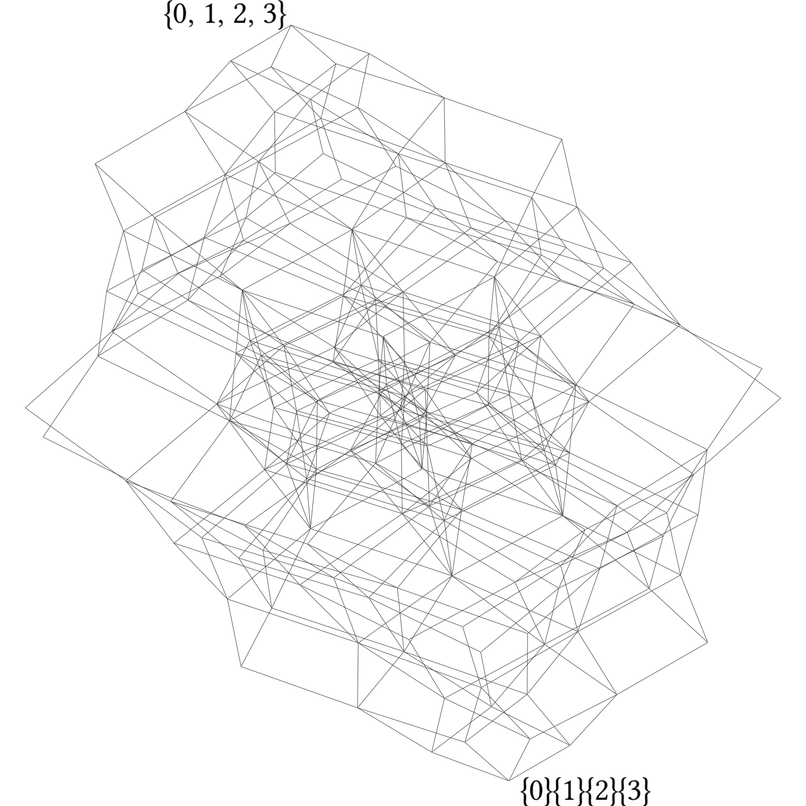
where represents the unique information carried by about , denotes the synergistic information available only from the joint state of the variables, and represents the redundant information about shared by and . To construct information sources from an arbitrary set of predictor variables, one should consider redundancies among all possible combinations of subsets of . However, note that the redundancy among a set and a set reduces to the unique information of if . This restricts the set of information sources to combinations of predictor subsets that are mutually incomparable by the ordering . Such incomparable sets are called antichains of the poset . Two antichains and can be ordered by redundancy by setting if for every there is an such that . That is, if contains at least the redundancy with respect to the outcome that does. The Hasse diagram of this lattice of antichains is shown in Figure 3 for up to . Note that the redundancy lattice is different from both the powerset and partition lattices, but is completely isomorphic up to variables (cf. Figures 1 and 2).
Let be the redundancy lattice of variables. The PID decomposition of the information that a set of variables carries about can then be written as
| (43) |
This can be inverted to get expressions of the individual contributions in terms of the mutual information :
| (44) |
This inversion, however, is far from trivial. One problem is that , where is the th Dedekind number. The series of Dedekind numbers grows so quickly that it is only known up to jakel2023computation ; van2023computation . This makes the Möbius inversion of the PID computationally infeasible for large , although a closed-form expression for the Möbius function on the redundancy lattice has recently been derived jansma2024decomposing .
However, even when the Möbius function can be calculated, this inversion leads to an ambiguity, as the definition of is unclear when the antichain contains more than a single set of variables. Consequently, solving the PID requires a well-defined notion of information on arbitrary antichains. A significant portion of the literature on the PID has focused on constructing such definitions, but no consensus has been reached thus far.
Recently, the PID framework has been extended to accommodate multiple target variables and information dynamics in time mediano2021towards . The associated ID decomposition lattice is the product of the standard redundancy lattices associated to the individual targets. Since the Möbius function of a product of lattices is the product of Möbius functions of the lattices stanley2011enumerative , the ID decomposition reduces to that of the normal PID when the Möbius function of the redundancy lattice is known.
III.3 Biology
III.3.1 Epistasis
In the last decade, improved genetic sequencing of genomes and transcriptomes has revealed that traits often depend on many, if not most genes. This change in perspective has been described as a transition from monogenic, to polygenic and omnigenic models boyle2017expanded . Furthermore, the effect of a single genetic variant can depend on the presence of other genetic variants, a type of genetic interaction called epistasis. As in the example of a person’s height in the introduction, a general phenotype that depends on the presence of a set of genetic variants can be decomposed into the sum of the effects of subsets of genetic variants. A Möbius inversion on the lattice of subsets of genetic variants gives the following definitions for genetic effects and epistatic interactions :
| (45) | ||||
| (46) | ||||
| That is, the interaction among a set of genes can be expressed in terms of observed phenotypes of individuals with varying genotypes. For example, the interaction among three genes is given by | ||||
| (47) | ||||
This expression is indeed the one used to estimate epistasis in much of the literature. The authors of beerenwinkel2007epistasis arrive at a similar expression based on volumes of polytopes, which has been used to describe epistasis among genetic variants eble2023master as well as in the context of microbiomes gould2018microbiome .
Even though interactions are necessarily defined with respect to some outcome, this need not be a phenotype in the traditional sense of the word. One possible outcome that requires no macroscopic measurements, for example, is the population probability of a particular gene expression pattern. If we represent gene expression as a binary vector , where if gene is expressed above some threshold, then inverting the log-probability of observing transcriptome gives the following definition of the interaction among genes :
| (48) |
which can be directly estimated from a population sample. A method to estimate such interactions from single-cell RNA-seq data was recently developed, and used to identify novel cell states and types in various organisms jansma2023high .
Instead of inferring the log-probability, i.e. the surprisal, one could also invert its expected value, i.e. the entropy. As explained in Section III.2, this yields (higher-order) mutual information, which is used by the algorithm that won the DREAM2 challenge of inferring gene regulatory networks from expression data watkinson2009inference .
III.3.2 Epidemiology
The central question in epidemiology is to understand the influence of various factors on an individual’s health outcomes. One obvious example is estimating the effect a vaccine has on disease risk. However, disease risk after vaccination is not only determined by the vaccine itself, but also by innate factors like the individual’s immune system and external factors like the presence of other pathogens, as well as interactions among these. Typically, the effect on outcome of a factor is isolated from all other factors by randomly dividing the population into groups, and then intervening such that in group 1, and in group 2. The Average Treatment Effect (ATE) is then defined as
| (49) |
However, in observational studies, where randomisation followed by intervention is not possible, the effect of generally cannot be isolated, and the outcome depends on a potentially large set of factors such that:
| (50) |
where now represents the effect of the collection of factors on the outcome . The effect of a single factor is then seen to be given by an ATE in the absence of any of the other factors:
| (51) | ||||
| whereas the second- and higher-order terms correspond to interactions among the factors, equivalent to the epidemiological interactions defined in beentjes2020higher . For example, the interaction among two factors is given by | ||||
| (52) | ||||
| (53) | ||||
In theory, this allows one to estimate drug interactions from population statistics.
III.3.3 Neuroscience
As biology tends to deal with very complex systems, decompositions are ubiquitous. The history of neuroscience can accordingly be described by evolving views on what the appropriate decomposition of the brain is: from neurons, to neural circuits, to hierarchical structures, to the currently popular approach that focuses on different spatial and functional regions bechtel2002decomposing . To describe the correlations and higher-order relationships between parts of the brain, both the classical approach to higher-order information theory, as well as the PID are commonly used, reflecting concurrent use of both the powerset and redundancy decomposition erramuzpe2015identification ; ince2017statistical ; wibral2017quantifying ; sherrill2021partial ; newman2022revealing
III.4 Physics
III.4.1 Equilibrium dynamics
Statistical physics is largely focused on relating the large-scale behaviour of a system to the microscopic interactions. Commonly, this is done through an energy function that maps a state of the system to its energy. Writing down a form of amounts to choosing a decomposition of the system into parts. For example, the Ising model assumes that the energy of a system , , decomposes into singleton and pairwise contributions and is given by
| (54) | |||
| or, for a subsystem | |||
| (55) | |||
where is the external field acting on spin and is the interaction strength between spins and , typically only nonzero for nearest neighbours on a lattice. Limiting the interactions to linear and pairwise quantities only is an assumption imposed by the Ising model. A more general form of the energy function would be
| (56) |
where is the interaction strength of the part and denotes the powerset of . If one is given the parameters , the forward problem is to calculate the behaviour of the system under the influence of the energy function . The inverse problem is to infer the parameters from observations of the system . The inverse problem is in general intractable, as direct observations of the energy are not possible. However, at equilibrium, the probability of observing a state is given by the Boltzmann distribution
| (57) |
where is the partition function. This means that one can observe the energy (up to an unimportant global shift) of a state indirectly as by simply estimating the probability of a state from a collection of samples. From this, a Möbius inversion quickly yields precise values for the parameters jansma2023higher :
| (58) | ||||
| (59) | ||||
| (60) |
For example, the inverse Ising problem for pairwise nearest-neighbour interactions at equilibrium is solved by
| (61) | ||||
| where denotes all spins except and . Simplifying notation further by writing , the 3-point coupling is given by | ||||
| (62) | ||||
This solution to the inverse problem was already noted in beentjes2020higher , but the argument presented here shows that the forward and inverse problem are exactly related through a Möbius inversion.
The chosen powerset decomposition of the energy function restricts this approach to binary variables. However, categorical variables can obey different partial orders but be treated in the same way, leading to a new notion of interaction that is no longer related to spin models. This construction is briefly discussed in beentjes2020higher ; jansma2023higher .
III.4.2 Statistical mechanics
In the approach above, one still needs access to observations of all microscopic variables to estimate the energy of observed states and solve the inverse problems. However, one could also start the line of reasoning from more macroscopic quantities, like averages over an ensemble. For example, one might only be able to measure the expected value of variables and their products, called correlation functions. For example, the two-point correlation function is given by
| (63) |
where the summation is over the full state space of the joint system . The observed correlations will be the result of microscopic interactions, but the exact form of the interactions might be unknown. To decompose the correlation function into contributions from individual interactions, it should be noted that to respect the multiplication rule of probability, contributions of multiple interactions happening in a single process should be multiplied. For this reason, a decomposition of a system of variables into products over partitions is most appropriate:
| (64) |
where is the set of all partitions of , and is the contribution by the members of partition element . For example, the 4-point correlation function can be decomposed into the following contributions, where variables that appear together in a given partition are connected by a line:
| (65) |
For example, a diagram like corresponds to a term , and might be interpreted as the contribution of the situation in which and interact, but and do not. The correlation functions can then be inverted over the lattice of partitions to give the contributions of individual diagrams, as well as those of terms involving a single . For example, the first three orders of are easily seen to be given by
| (66) | ||||
| (67) | ||||
| (68) |
These are exactly the famous Ursell functions of statistical mechanics. Ursell functions are also called connected correlation functions, because a single term involves only the connected part of a diagram in the expansion of Equation (65). While the first three Ursell functions coincide with the mixed central moments, the higher-order Ursell functions are different, and used throughout statistical mechanics. The Ursell functions are related to the higher-order interactions of the theory and are essentially the cumulants of the dynamics, which is why they rely on exactly the same decomposition of moments as was described in Section III.1. Note, however, that Ursell functions are the partition-inverse of the moments, while the higher-order interactions of equilibrium dynamics are the powerset-inverse of the energy.
III.4.3 Quantum & Statistical Field Theory
In quantum field theory, the random variables are replaced by field operators . The correlation functions—or Green’s functions—are then defined as expectation values of time-ordered products of field operators in the vacuum state :
| (69) | ||||
| (70) |
where is the time-ordering operator, is the action of the field theory, , and the integral is over all possible field configurations. The reason that such time-ordered correlation functions are of great interest, is that they determine the particle scattering amplitudes in a given quantum field theory through the LSZ reduction formula lehmann1955formulierung ; peskin2018introduction . To calculate the correlation functions, one typically introduces a functional , defined as
| (71) | ||||
| such that | ||||
| (72) | ||||
where is the functional derivative with respect to . The functional can be expanded in a power series in , and the coefficients of this expansion are the correlation functions, which is why is called the generating functional, in analogy with the moment generating function of probability theory. Note, however, that the analogy is not perfect: correlation functions are complex-valued, and are not defined with respect to a joint distribution over states so cannot be interpreted as the moments of a probability distribution.
Now, as in the case of statistical classical mechanics, one might decompose the quantum correlation functions over the lattice of partitions:
| (73) |
where the are the contributions of the members of the partition element . This can of course be represented by the same diagrams as in the case of statistical mechanics in Equation 65, but there is an important difference. By expanding as a power series around the non-interacting theory up to certain order and applying Wick’s theorem to the resulting products of operators, one can show that the connected correlation functions are given by the sum of all Feynman diagrams with the same external vertices, but with an arbitrary number of internal vertices and loops. To emphasise that the diagrammatic representations of the deomposition may contain arbitrary internal processes, we draw the quantum diagrams with a shaded internal circle:
A single connected component of one of the diagrams now represents an infinite sum over Feynman diagrams. For example, in a theory with quartic interactions:
| (74) |
A Möbius inversion on the lattice of partitions then gives an expression for the connected components of these graphs in terms of the correlation functions. For example:
| (75) | ||||
| (76) | ||||
| (77) | ||||
| (78) |
The expansion of a quantum amplitude associated to a scattering process only involves such diagrams where all external lines are connected, so for any given quantum field theory, one can identify scattering amplitudes as the Möbius inverse of correlation functions on the lattice of partitions.
It should be emphasised that while we used the language of quantum field theory throughout this section, similar methods lead to definitions of cumulants in classical- and mean-field theories as well. In fact, classical statistical field theory is directly related to quantum field theory through a Wick rotation (by replacing imaginary time by inverse temperature). While there is a strong analogy to the decomposition of the moments in Section III.1, it should be emphasised that the correlation functions treated here are not the moments of some probability distribution over field configurations. Rather, the analogy holds only at the level of the expectation values, and the fact that one can define a moment generating function , as well as a cumulant generating function . This fact has been used for decades to define cumulants in any setting where a suitable notion of average can be defined, and is known as the generalised cumulant expansion method kubo1962generalized . Such approaches have been used to define connected correlations in networks of neurons ocker2017linking , on belief propagation graphs chertkov2006loop ; welling2012cluster , and in chemical dynamics domb1972cluster ; klein1999chemical .
III.5 Chemistry
A significant challenge in chemistry is predicting the properties of molecules from their configuration, commonly referred to as the quantitative structure-activity relationship (QSAR). To describe a molecular property in terms of the configuration of a molecule , one might associate a graph with the molecule, where the nodes are atoms and the edges are bonds. The property can then be expressed as a function of the subgraphs of :
| (79) |
where is the contribution of the subgraph to the property and the sum is over all subgraphs of . A straightforward Möbius inversion is of course possible, but some chemical properties are more naturally decomposed over other posets. For example, a molecule’s resonance energy is most naturally decomposed into contributions from acyclic graphs only. Motivated such chemical questions, the authors of babic1996mobius derived a closed-form expression for the Möbius function on this poset of acyclic graphs.
Also studied in chemistry is how properties of a family of molecules are related. The authors of ivanciuc2005posetic , for instance, study how toxic molecules from the family of Chlorobenzenes are to guppies. A chlorobenzene is a benzene molecule where one or more hydrogen atoms have been replaced by chlorine atoms. That means that there is a certain partial order one can impose on the set of 13 possible chlorobenzenes (taking into account the 6-fold rotational symmetry of the benzene ring). Namely, two chlorobenzenes and are related by if can be created from by adding a single chlorine atom. The toxicity can then be expressed as a sum over the toxic contributions of the chlorobenzenes that come before it in the reaction chain:
| (80) |
Similarly, the authors of ivanciuc2007posetic construct the poset of adding methyl groups to cyclobutanes. As the molecules higher-up in the partial order are constructed from the lower ones, one could expand the property of a molecule in terms of the contributions of the molecules that come before it. This means that every molecule defines its own poset and thus Möbius function, but these have been calculated and used to verify that higher-order contributions decrease so that truncating the expansion at a certain level leads to a good approximation of the property ivanciuc2007posetic .
III.6 Game Theory
In coalitional game theory, players can form coalitions and cooperate, potentially increasing their expected payoff. The core idea is that value might add synergistically, or superadditively. For example, a pair of shoes might be worth more than twice the value of an individual shoe. Therefore, one could decompose the total value of a coalition into the sum of the synergistic contributions of all subsets of :
| (81) |
If the value of the coalitions is known, then this can be inverted on the Boolean algebra of subsets of to yield a definition of the synergistic contributions :
| (82) |
One reason that exact values for the synergy of coalitions might be relevant, is that they are a natural answer to the question of how to distribute the value of a coalition among its members. Since the synergy of a given coalition cannot be attributed to any single member, it should be distributed evenly among all members. The payout any individual player should then expect in a grand coalition involving all of players is then the average synergy that player adds to each possible coalition that includes them:
| (83) |
This is a very well-known quantity, known as the Shapley value for player . It is more commonly written as
| (84) |
and is the unique payout function that satisfies a number of favourable properties. In other words: the Shapley value of a player is the Möbius inverse of the normalised synergy of a coalition on the inclusion lattice of subsets of that include .
Choosing a different normalisation in the decomposition of , one that for example depends on the identity of player , the Möbius inversion recovers a family of distribution rules billot2005share .
III.7 Artificial Intelligence
Modern artificial intelligence systems are complex and involve many interacting parts. While the practical and commercial success of machine learning models has been undeniable, a good understanding of the relationship between the microscopic structure of the model and its emergent macroscopic behaviour is still lacking in most applications. In many situations, like medical applications, a way to link the microscopic structure of a model to its macroscopic behaviour is a crucial step towards widespread adoption.
Predictive machine learning models are generally trained on many features, but once the final model has been constructed it can be difficult to determine how much each feature contributes to the prediction. One way to address this issue is to decompose the prediction of the model into contributions of individual features, and using the Shapley value to assign a total contribution to each feature, replacing the value function with the model’s prediction, and marginalising over the features not in cohen2007feature ; williamson2020efficient ; fryer2021shapley . This allows one to determine which features are most important for a particular model’s prediction, as well as which groups of features show synergistic effects.
In generative machine learning, the features do not contribute to a prediction, but to a probability distribution. Since energy-based models have a closed-form expression for the generated probability distribution, they allow for a precise understanding of the relationship between their internal structure and the encoded distribution. One architecture that has led to particularlty fruitful insights has been the Restricted Boltzmann machine, in which the probability of a sample is essentially the Boltzmann distribution of a statistical physics model. An argument similar as above reveals that the cumulants of the model are the Möbius inverse of the mixed moments of the model and describe the interactions among the features, with higher-order interactions corresponding to synergistic effects among the features nguyen2017inverse ; cossu2019machine ; jansma2023higher .
Even before the modern success of machine learning techniques, artificial intelligence has created formal methods to treat reasoning agents. Dempster-Shafer theory is a generalisation of Bayesian probability theory dempster1967upper ; shafer1976mathematical (though its precise relationship to Bayesian inference is controversial dezert2013dempster ) that formalises how agents combine evidence to update beliefs. It decomposes the set of all properties of the universe into the powerset of propositions about . Each element (A) from the powerset then gets assigned a certain belief mass through the basic belief assignment function , where . The total belief an agent has about a proposition is then given by the mass of and the mass of all subsets of
| (85) | |||
| such that the belief assignment function can be expressed in terms of the belief of agents after observing varying evidence | |||
| (86) | |||
which is used to define the generalised Bayesian update rule. While classical Dempster-Shafer theory always used the powerset decomposition, more modern approaches have generalised this to other lattices where properties of the Möbius function are known grabisch2009belief ; zhou2013belief .
IV Discussion
| Field of Study | Macro Quantity | Decomposition | Micro Quantity/Interactions |
|---|---|---|---|
| Statistics | Moments | Powerset | Central moments |
| Moments | Partitions | Cumulants | |
| Free moments | Non-crossing partitions | Free cumulants | |
| Path signature moments | Ordered partitions | Path signature cumulants | |
| Information Theory | Entropy | Powerset | Mutual information |
| Surprisal | Powerset | Pointwise mutual information | |
| Joint Surprisal | Powerset | Conditional interactions | |
| Mutual Information | Antichains | Synergy/redundancy atoms | |
| Biology | Pheno- & Genotype | Powerset | Epistasis |
| Gene expression profile | Powerset | Genetic interactions | |
| Population statistics | Powerset | Synergistic treatment effects | |
| Physics | Ensemble energies | Powerset | Ising interactions |
| Correlation functions | Partitions | Ursell functions | |
| Quantum corr. functions | Partitions | Scattering amplitudes | |
| Chemistry | Molecular property | Subgraphs | Fragment contributions |
| Molecular property | Reaction poset | Cluster contributions | |
| Game Theory | Coalition value | Powerset | Coalition synergy |
| Shapley value | Powerset | Normalised coalition synergy | |
| Artificial intelligence | Generative model probabilities | Powerset | Feature interactions |
| Predictive model predictions | Powerset | Feature contributions | |
| Dempster-Shafer Belief | Distributive | Evidence weight |
The aim of this study has been to provide a unified perspective on the various notions of higher-order interactions in complex systems. We have shown that decomposing a system into parts leads to a unique definition of the interactions among the parts, through a Möbius inversion of the outcome of interest. We found that this approach reproduces well-known notions of higher-order structure in a variety of scientific fields, an overview of which is provided in Table 1. While some of the relationships in Table 1 have previously been described as Möbius inversions, to our knowledge this is the first time that the shared structure underlying these definitions has been made explicit.
The presented framework shows how the choice of system decomposition determines the nature of the derived interactions. This highlights decomposition selection as a key step in studying complex system behaviour. While there are no universal criteria for a ”good” decomposition, in each case the decomposition should be motivated by knowledge of the system’s structure and the macroscopic property of interest. For example, a partition-based decomposition may be natural when the property depends on how different parts come together, while a powerset-based decomposition is more suited to properties that depend binary configurations of the parts.
Fundamentally, this framework mathematises the notion that complex system properties depend on the way the system is carved up into parts. Different decompositions reveal different kinds of interactions; there is no single, privileged decomposition. The ”correct” decomposition is the one that yields meaningful interactions for the question of interest, as seen in the various examples.
One way to interpret the Möbius inversion theorem is as a relationship between the macro- and microscopic degrees of freedom of a system. If , then since is the sum of contributions of all parts, it can be considered a macroscopic feature of the system. The Möbius inversion theorem then states that the microscopic contributions can be recovered from the macroscopic feature observed on the parts. In this sense, it provides a way to study the emergent properties of complex systems, but it should be emphasised that the inversion is only possible if the macroscopic quantity is also defined for the smaller parts. For many classic examples of emergence, like bird flocks, temperature, etc, this is not possible.
An interesting example of this problem arose in the partial information decomposition. With the decomposition defined on the redundancy lattice of antichains, estimating the contribution of the information atoms is only possible given a suitable notion of redundant information on each of the antichains. Much of the PID literature has focused on resolving this ambiguity in different ways, but no concensus has been reached so far. However, this also highlights how versatile the Möbius inversion framework is: even when the decomposition results in ambiguity, different resolutions of this ambiguity can give rise to a rich set of higher-order structure, which in the case of the PID have been used to characterise different properties of neural information processing wibral2017quantifying ; sherrill2021partial ; luppi2022synergistic .
As a general rule, observations of a system provide access to the macroscopic features (moments, phenotypes, energies, predictions, etc), which can then be used to infer the microscopic interactions (cumulants, genetic interactions, Ising interactions, feature contributions, etc), so the Möbius inversion theorem is essentially a solution to the inverse problem of inferring microscopic structure from macroscopic observables. Note, however, that it solves the inverse problem relative to a chosen decomposition. If the chosen decomposition is not appropriate, then the Möbius inversion theorem will not provide a meaningful interpretation of the microscopic interactions either. One example of this is the Möbius inversion on the lattice of partitions that related scattering amplitudes of quantum field theory to correlation functions. The Möbius inversion still gave infinite sums over Feynman diagrams, not the contribution of individual diagrams, so the microscopic interactions were not directly accessible from the macroscopic observables. Furthermore, collections of particles can carry more structure, like fermion number and colour, which also implies that partitions are not the most appropriate decomposition for the problem.
One interesting phenomenon not explored in the present study is that of lattice dualities. It was observed in jansma2023higher that since the order-theoretic dual of a lattice is again a lattice, there are dual higher-order structures implied by a given decomposition lattice. In information theory, the dual to information theory was found to be conditional mutual information, with a similar dual quantity derived for Ising interactions. It is an unexplored but interesting question whether the quantities dual to the ones presented here also offer a meaningful interpretation, but this is left for future work.
Another exciting direction for future work is to use the current framework to transfer insights from one scientific discipline to another. For example, in the so-called cluster variation method, physical intuition has motivated the truncation of sums over lattice subsets to obtain approximations to thermodynamic quantities of crystals kikuchi1951theory . This summation can be seen as a truncated Möbius inversion over the lattice of physical crystal lattice sites an1988note ; morita1990cluster , and could be explored as an approximation scheme in other settings as well. In fact, precisely such a truncation has been suggested in decompositions of chemical properties of molecules ivanciuc2007posetic . In addition, the authors of jansma2023high use causal discovery methods to improve the estimation of genetic interactions (the Möbius inverse of gene-expression profiles). Since the estimation of microscopic interactions from macroscopic observables can require many observations, similar methods could be used to improve the estimability of higher-order interactions in other fields.
Other future work could explore different kinds of decompositions and the higher-order structure they imply. For example, a recent study has started to explore the combinatorics of nucleotide sequences in polyploid genomes by decomposing sequencing data over the lattice of integer partitions ordered by refinement ranallo2020genomescope . More speculatively, decompositions beyond locally finite partial orders could be explored by suitably generalising the Möbius inversion theorem. It is well-known that the Möbius inversion theorem can be generalised to a more general class of skeletal categories that includes not just posets but also monoids and groupoids content1980categories ; leinster2012notions . Whether these more general decompositions faithfully and fruitfully describe higher-order structure in complex systems is, to our best knowledge, a mostly unexplored and open question. We hope that this work inspires others to explore novel decompositions and discover new types of higher-order structures in complex systems.
Acknowledgements
The connections to game theory, chemistry, and path statistics were the result of fruitful discussions with Jürgen Jost, Guillermo Restrepo, and Darrick Lee, respectively. The author is also grateful to Eckehard Olbrich and Fernando Rosas for insightful discussions on the partial information decomposition, as well as to Hadleigh Frost for his comments on diagrammatic sums in quantum field theory.
References
- [1] G. An. A note on the cluster variation method. Journal of Statistical Physics, 52:727–734, 1988.
- [2] Y. E. Antebi, J. M. Linton, H. Klumpe, B. Bintu, M. Gong, C. Su, R. McCardell, and M. B. Elowitz. Combinatorial signal perception in the bmp pathway. Cell, 170(6):1184–1196, 2017.
- [3] D. N. Arnosti, S. Barolo, M. Levine, and S. Small. The eve stripe 2 enhancer employs multiple modes of transcriptional synergy. Development, 122(1):205–214, 1996.
- [4] N. Ay, E. Olbrich, N. Bertschinger, and J. Jost. A geometric approach to complexity. Chaos: An Interdisciplinary Journal of Nonlinear Science, 21(3), 2011.
- [5] D. Babić and N. Trinajstić. Möbius inversion on a poset of a graph and its acyclic subgraphs. Discrete applied mathematics, 67(1-3):5–11, 1996.
- [6] F. Battiston, E. Amico, A. Barrat, G. Bianconi, G. Ferraz de Arruda, B. Franceschiello, I. Iacopini, S. Kéfi, V. Latora, Y. Moreno, et al. The physics of higher-order interactions in complex systems. Nature Physics, 17(10):1093–1098, 2021.
- [7] W. Bechtel. Decomposing the mind-brain: A long-term pursuit. Brain and Mind, 3:229–242, 2002.
- [8] S. V. Beentjes and A. Khamseh. Higher-order interactions in statistical physics and machine learning: A model-independent solution to the inverse problem at equilibrium. Physical Review E, 102(5):053314, 2020.
- [9] N. Beerenwinkel, L. Pachter, and B. Sturmfels. Epistasis and shapes of fitness landscapes. Statistica Sinica, pages 1317–1342, 2007.
- [10] A. Billot and J.-F. Thisse. How to share when context matters: The möbius value as a generalized solution for cooperative games. Journal of Mathematical Economics, 41(8):1007–1029, 2005.
- [11] P. Bonnier and H. Oberhauser. Signature cumulants, ordered partitions, and independence of stochastic processes. 2020.
- [12] S. P. Borgatti, A. Mehra, D. J. Brass, and G. Labianca. Network analysis in the social sciences. science, 323(5916):892–895, 2009.
- [13] E. A. Boyle, Y. I. Li, and J. K. Pritchard. An expanded view of complex traits: from polygenic to omnigenic. Cell, 169(7):1177–1186, 2017.
- [14] M. Chertkov and V. Y. Chernyak. Loop series for discrete statistical models on graphs. Journal of Statistical Mechanics: Theory and Experiment, 2006(06):P06009, 2006.
- [15] S. Cohen, G. Dror, and E. Ruppin. Feature selection via coalitional game theory. Neural computation, 19(7):1939–1961, 2007.
- [16] M. Content, F. Lemay, and P. Leroux. Catégories de möbius et fonctorialités: un cadre général pour l’inversion de möbius. Journal of Combinatorial Theory, Series A, 28(2):169–190, 1980.
- [17] G. Cossu, L. Del Debbio, T. Giani, A. Khamseh, and M. Wilson. Machine learning determination of dynamical parameters: The ising model case. Physical Review B, 100(6):064304, 2019.
- [18] A. Dempster. Upper and lower probabilities induced by a multi-valued mapping. Annals of Mathematical Statistics, 38, 1967.
- [19] D. C. Dennett. Darwin’s dangerous idea. The Sciences, 35(3):34–40, 1995.
- [20] J. Dezert, A. Tchamova, D. Han, and J.-M. Tacnet. Why dempster’s fusion rule is not a generalization of bayes fusion rule. In Proceedings of the 16th International Conference on Information Fusion, pages 1127–1134. IEEE, 2013.
- [21] C. Domb and G. Joyce. Cluster expansion for a polymer chain. Journal of Physics C: Solid State Physics, 5(9):956, 1972.
- [22] H. Eble, M. Joswig, L. Lamberti, and W. B. Ludington. Master regulators of biological systems in higher dimensions. Proceedings of the National Academy of Sciences, 120(51):e2300634120, 2023.
- [23] M. Eidi and J. Jost. Ollivier ricci curvature of directed hypergraphs. Scientific Reports, 10(1):12466, 2020.
- [24] A. Erramuzpe, G. J. Ortega, J. Pastor, R. G. De Sola, D. Marinazzo, S. Stramaglia, and J. M. Cortes. Identification of redundant and synergetic circuits in triplets of electrophysiological data. Journal of neural engineering, 12(6):066007, 2015.
- [25] J. W. Essam. Graph theory and statistical physics. Discrete Mathematics, 1(1):83–112, 1971.
- [26] D. Fryer, I. Strümke, and H. Nguyen. Shapley values for feature selection: The good, the bad, and the axioms. Ieee Access, 9:144352–144360, 2021.
- [27] E. Gardner. Spin glasses with p-spin interactions. Nuclear Physics B, 257:747–765, 1985.
- [28] G. Ghoshal, V. Zlatić, G. Caldarelli, and M. E. Newman. Random hypergraphs and their applications. Physical Review E, 79(6):066118, 2009.
- [29] A. L. Gould, V. Zhang, L. Lamberti, E. W. Jones, B. Obadia, N. Korasidis, A. Gavryushkin, J. M. Carlson, N. Beerenwinkel, and W. B. Ludington. Microbiome interactions shape host fitness. Proceedings of the National Academy of Sciences, 115(51):E11951–E11960, 2018.
- [30] M. Grabisch. Belief functions on lattices. International Journal of Intelligent Systems, 24(1):76–95, 2009.
- [31] M. Grandjean. A social network analysis of twitter: Mapping the digital humanities community. Cogent Arts & Humanities, 3(1):1171458, 2016.
- [32] G. M. Hodgson. Generalizing darwinism to social evolution: Some early attempts. Journal of Economic Issues, 39(4):899–914, 2005.
- [33] R. A. Ince, B. L. Giordano, C. Kayser, G. A. Rousselet, J. Gross, and P. G. Schyns. A statistical framework for neuroimaging data analysis based on mutual information estimated via a gaussian copula. Human brain mapping, 38(3):1541–1573, 2017.
- [34] T. Ivanciuc, O. Ivanciuc, and D. J. Klein. Posetic quantitative superstructure/activity relationships (qssars) for chlorobenzenes. Journal of chemical information and modeling, 45(4):870–879, 2005.
- [35] T. Ivanciuc, D. J. Klein, and O. Ivanciuc. Posetic cluster expansion for substitution-reaction networks and application to methylated cyclobutanes. Journal of Mathematical Chemistry, 41:355–379, 2007.
- [36] C. Jäkel. A computation of the ninth dedekind number. arXiv preprint arXiv:2304.00895, 2023.
- [37] A. Jansma. Higher-order interactions and their duals reveal synergy and logical dependence beyond shannon-information. Entropy, 25(4):648, 2023.
- [38] A. Jansma. Higher-order interactions in single-cell gene expression. PhD thesis, University of Edinburgh, 2023.
- [39] A. Jansma and F. E. Rosas. Decomposing information on the free distributive lattice (forthcoming). 2024.
- [40] A. Jansma, Y. Yao, J. Wolfe, L. Del Debbio, S. V. Beentjes, C. P. Ponting, and A. Khamseh. High order expression dependencies finely resolve cryptic states and subtypes in single cell data. bioRxiv, pages 2023–12, 2023.
- [41] E. T. Jaynes. Information theory and statistical mechanics. Physical review, 106(4):620, 1957.
- [42] R. Kikuchi. A theory of cooperative phenomena. Physical review, 81(6):988, 1951.
- [43] T. R. Kirkpatrick and D. Thirumalai. p-spin-interaction spin-glass models: Connections with the structural glass problem. Physical Review B, 36(10):5388, 1987.
- [44] D. Klein, T. Schmalz, and L. Bytautas. Chemical sub-structural cluster expansions for molecular properties. SAR and QSAR in Environmental Research, 10(2-3):131–156, 1999.
- [45] H. E. Klumpe, M. A. Langley, J. M. Linton, C. J. Su, Y. E. Antebi, and M. B. Elowitz. The context-dependent, combinatorial logic of bmp signaling. Cell systems, 13(5):388–407, 2022.
- [46] R. Kubo. Generalized cumulant expansion method. Journal of the Physical Society of Japan, 17(7):1100–1120, 1962.
- [47] E. Kuzmin, B. VanderSluis, W. Wang, G. Tan, R. Deshpande, Y. Chen, M. Usaj, A. Balint, M. Mattiazzi Usaj, J. Van Leeuwen, et al. Systematic analysis of complex genetic interactions. Science, 360(6386):eaao1729, 2018.
- [48] L. Lang, P. Baudot, R. Quax, and P. Forré. Information decomposition diagrams applied beyond shannon entropy: A generalization of hu’s theorem. arXiv preprint arXiv:2202.09393, 2022.
- [49] W. Leal, G. Restrepo, P. F. Stadler, and J. Jost. Forman–ricci curvature for hypergraphs. Advances in Complex Systems, 24(01):2150003, 2021.
- [50] H. Lehmann, K. Symanzik, and W. Zimmermann. Zur formulierung quantisierter feldtheorien. Il Nuovo Cimento (1955-1965), 1:205–225, 1955.
- [51] T. Leinster. Notions of möbius inversion. Bulletin of the Belgian Mathematical Society-Simon Stevin, 19(5):909–933, 2012.
- [52] Q. F. Lotito, F. Musciotto, A. Montresor, and F. Battiston. Higher-order motif analysis in hypergraphs. Communications Physics, 5(1):79, 2022.
- [53] A. I. Luppi, P. A. Mediano, F. E. Rosas, N. Holland, T. D. Fryer, J. T. O’Brien, J. B. Rowe, D. K. Menon, D. Bor, and E. A. Stamatakis. A synergistic core for human brain evolution and cognition. Nature Neuroscience, 25(6):771–782, 2022.
- [54] H. J. Maris and L. P. Kadanoff. Teaching the renormalization group. American journal of physics, 46(6):652–657, 1978.
- [55] O. Mason and M. Verwoerd. Graph theory and networks in biology. IET systems biology, 1(2):89–119, 2007.
- [56] P. A. Mediano, F. E. Rosas, A. I. Luppi, R. L. Carhart-Harris, D. Bor, A. K. Seth, and A. B. Barrett. Towards an extended taxonomy of information dynamics via integrated information decomposition. arXiv preprint arXiv:2109.13186, 2021.
- [57] L. Merchan and I. Nemenman. On the sufficiency of pairwise interactions in maximum entropy models of networks. Journal of Statistical Physics, 162:1294–1308, 2016.
- [58] T. Morita. Cluster variation method and möbius inversion formula. Journal of Statistical Physics, 59:819–825, 1990.
- [59] E. L. Newman, T. F. Varley, V. K. Parakkattu, S. P. Sherrill, and J. M. Beggs. Revealing the dynamics of neural information processing with multivariate information decomposition. Entropy, 24(7):930, 2022.
- [60] H. C. Nguyen, R. Zecchina, and J. Berg. Inverse statistical problems: from the inverse ising problem to data science. Advances in Physics, 66(3):197–261, 2017.
- [61] G. K. Ocker, K. Josić, E. Shea-Brown, and M. A. Buice. Linking structure and activity in nonlinear spiking networks. PLoS computational biology, 13(6):e1005583, 2017.
- [62] G. A. Pavlopoulos, M. Secrier, C. N. Moschopoulos, T. G. Soldatos, S. Kossida, J. Aerts, R. Schneider, and P. G. Bagos. Using graph theory to analyze biological networks. BioData mining, 4:1–27, 2011.
- [63] M. E. Peskin. An introduction to quantum field theory. CRC press, 2018.
- [64] Plato. Phaedrus 265e. http://data.perseus.org/citations/urn:cts:greekLit:tlg0059.tlg012.perseus-eng1:265e, 370 BC.
- [65] T. R. Ranallo-Benavidez, K. S. Jaron, and M. C. Schatz. Genomescope 2.0 and smudgeplot for reference-free profiling of polyploid genomes. Nature communications, 11(1):1432, 2020.
- [66] R. Rosen. Some results in graph theory and their application to abstract relational biology. The bulletin of mathematical biophysics, 25(2):231–241, 1963.
- [67] G.-C. Rota. On the foundations of combinatorial theory i. theory of möbius functions. Zeitschrift für Wahrscheinlichkeitstheorie und verwandte Gebiete, 2(4):340–368, 1964.
- [68] G.-C. Rota and J. Shen. On the combinatorics of cumulants. Journal of Combinatorial Theory, Series A, 91(1-2):283–304, 2000.
- [69] H. Schawe and L. Hernández. Higher order interactions destroy phase transitions in deffuant opinion dynamics model. Communications Physics, 5(1):32, 2022.
- [70] M. Scheffer, J. Bascompte, W. A. Brock, V. Brovkin, S. R. Carpenter, V. Dakos, H. Held, E. H. Van Nes, M. Rietkerk, and G. Sugihara. Early-warning signals for critical transitions. Nature, 461(7260):53–59, 2009.
- [71] G. Shafer. A mathematical theory of evidence, volume 42. Princeton university press, 1976.
- [72] S. P. Sherrill, N. M. Timme, J. M. Beggs, and E. L. Newman. Partial information decomposition reveals that synergistic neural integration is greater downstream of recurrent information flow in organotypic cortical cultures. PLoS computational biology, 17(7):e1009196, 2021.
- [73] P. S. Skardal and A. Arenas. Higher order interactions in complex networks of phase oscillators promote abrupt synchronization switching. Communications Physics, 3(1):218, 2020.
- [74] R. Solé. Phase transitions, volume 3. Princeton University Press, 2011.
- [75] T. Speed and H. Silcock. Cumulants and partition lattices v. calculating generalized k-statistics. Journal of the Australian Mathematical Society, 44(2):171–196, 1988.
- [76] R. Speicher. Free probability theory and non-crossing partitions. Séminaire Lotharingien de Combinatoire [electronic only], 39:B39c–38, 1997.
- [77] T. Spribille, V. Tuovinen, P. Resl, D. Vanderpool, H. Wolinski, M. C. Aime, K. Schneider, E. Stabentheiner, M. Toome-Heller, G. Thor, et al. Basidiomycete yeasts in the cortex of ascomycete macrolichens. Science, 353(6298):488–492, 2016.
- [78] R. P. Stanley. Enumerative combinatorics volume 1 second edition. Cambridge studies in advanced mathematics, 2011.
- [79] T. Tanaka and T. Aoyagi. Multistable attractors in a network of phase oscillators with three-body interactions. Physical Review Letters, 106(22):224101, 2011.
- [80] G. Tkacik, E. Schneidman, M. J. Berry II, and W. Bialek. Ising models for networks of real neurons. arXiv preprint q-bio/0611072, 2006.
- [81] L. Van Hirtum, P. De Causmaecker, J. Goemaere, T. Kenter, H. Riebler, M. Lass, and C. Plessl. A computation of d (9) using fpga supercomputing. arXiv preprint arXiv:2304.03039, 2023.
- [82] J. Watkinson, K.-c. Liang, X. Wang, T. Zheng, and D. Anastassiou. Inference of regulatory gene interactions from expression data using three-way mutual information. Annals of the New York Academy of Sciences, 1158(1):302–313, 2009.
- [83] D. J. Watts and S. H. Strogatz. Collective dynamics of ’small-world’ networks. nature, 393(6684):440–442, 1998.
- [84] S. Weinberg. The quantum theory of fields, volume 2. Cambridge university press, 1995.
- [85] M. Welling, A. E. Gelfand, and A. T. Ihler. A cluster-cumulant expansion at the fixed points of belief propagation. arXiv preprint arXiv:1210.4916, 2012.
- [86] M. Wibral, C. Finn, P. Wollstadt, J. T. Lizier, and V. Priesemann. Quantifying information modification in developing neural networks via partial information decomposition. Entropy, 19(9):494, 2017.
- [87] P. L. Williams and R. D. Beer. Nonnegative decomposition of multivariate information. arXiv preprint arXiv:1004.2515, 2010.
- [88] B. Williamson and J. Feng. Efficient nonparametric statistical inference on population feature importance using shapley values. In International conference on machine learning, pages 10282–10291. PMLR, 2020.
- [89] R. W. Yeung. A new outlook on shannon’s information measures. IEEE transactions on information theory, 37(3):466–474, 1991.
- [90] C. Zhou. Belief functions on distributive lattices. Artificial Intelligence, 201:1–31, 2013.
- [91] W. H. Zurek. Quantum darwinism. Nature physics, 5(3):181–188, 2009.