Transitions and Thermodynamics on Species Graphs of
Chemical Reaction Networks
Abstract
Chemical reaction networks (CRNs) exhibit complex dynamics governed by their underlying network structure. In this paper, we propose a novel approach to study the dynamics of CRNs by representing them on species graphs (S-graphs). By scaling concentrations by conservation laws, we obtain a graph representation of transitions compatible with the S-graph, which allows us to treat the dynamics in CRNs as transitions between chemicals. We also define thermodynamic-like quantities on the S-graph from the introduced transitions and investigate their properties, including the relationship between specieswise forces, activities, and conventional thermodynamic quantities. Remarkably, we demonstrate that this formulation can be developed for a class of irreversible CRNs, while for reversible CRNs, it is related to conventional thermodynamic quantities associated with reactions. The behavior of these specieswise quantities is numerically validated using an oscillating system (Brusselator). Our work provides a novel methodology for studying dynamics on S-graphs, paving the way for a deeper understanding of the intricate interplay between the structure and dynamics of chemical reaction networks.
I Introduction.
The theoretical framework of chemical reaction network (CRNs for short) is applied in various research fields, such as steady-state flux analysis in metabolic systems [1] and modeling non-equilibrium processes like oscillatory phenomena [2]. To investigate the properties that hold in a broad range of processes in CRNs, including non-equilibrium states, thermodynamic approaches have recently been used [3, 4]. Mathematically, CRNs possess a geometric structure represented by hypergraphs with stoichiometric information [5], whose structural constraints govern the behaviour of chemical reaction dynamics, for example, the controllability of chemical reactions [6].
For large-scale CRNs, the species graph approach has been utilized. This is due to the difficulty in intuitively understanding transitions between chemical species over the hypergraph structure, as well as the fact that graph-based characterisations such as small-world and scale-free properties for graphs are relatively well established [7, 8]. With this background, graph-based studies using species graphs (S-graph) or reaction graphs [9] are often preferred over hypergraphs for large networks such as metabolic systems [10, 11].
However, the dynamics corresponding to the S-graph have not been extensively explored. Despite the potential importance of dynamical oscillations in actual metabolic and glycolytic systems [12, 13], the dynamical aspects of species transitions in chemical reaction systems have been neglected.
In this paper, through scaling concentrations by conservation laws, we obtained a graph representation of transitions compatible with the S-graphs of chemical reaction networks. This transition representation enabled us to derive a novel thermodynamics-like formulation for CRNs. Remarkably, we demonstrated that this thermodynamics-like formulation can be applied to a class of irreversible CRNs, while to reversible CRNs, it is reduced to conventional thermodynamic quantities associated with reactions. A key contribution of our research is proposing a methodology to derive a master equation on the S-graph governing the scaled concentrations from deterministic CRN dynamics. Our work provides a novel approach to study of dynamics on S-graphs, paving the way for a deeper understanding of the intricate interplay between the structure and dynamics of chemical reaction networks.
The paper is structured as follows: The following section II introduces fundamental terms related to the CRN dynamics and note thermodynamic quantities defined in a reversible CRN. In the section III, we define a new physical quantity called ”transition” and reinterpret the CRN dynamics as dynamics on a species graph. The conservative nature of the dynamics on the graph is realised through concentration scaling by the conservation laws of the network. In the section IV, we define thermodynamic quantities on the species graph from the transitions we have introduced and investigate their properties. In particular, we discuss the relationship of the specieswise forces and activities with conventional thermodynamic quantities. The behaviour of the specieswise quantities is checked numerically using an oscillating system (Brusselator) in the section V.

II Foundation of chemical reaction network.
Fundamentals of chemical reaction networks and kinetics are reviewed in this section. The detailed notations can be found in [14, 15].
II.1 Notation and Preliminaries
Consider a non empty finite set of species. Let be a finite set of complexes. Suppose a non empty finite set of reactions satisfying the following conditions,
| (1) | |||||
| (2) |
We denote a reaction as . For a complex , its support is defined as . and are respectively called reactant and product complexes of a reaction . Each respectively represents a set of reactants and products. The triple of species, complexes and reactions is called a chemical reaction network (CRN) if satisfies the above conditions.
We distinguish proper reactions , which have and , import reactions for which , and export reactions for which . A CRN is closed if all reactions are proper. We focus on a closed CRN , unless explicitly stated otherwise.
Consider -norm on a complex set of ; for a complex , . The non-emptiness of a complex’s support is equivalent to the positiveness of its norm; . In the same way, properness of a reaction is represented in terms of its support or norm,
| (3) | |||||
| (4) | |||||
| (5) |
In this paper, () is called a total reactant (product) coefficient of a reaction . When a reaction has the same value of its two total coefficients , the value is simply called a total coefficient or degree of .
In our notation, the directed graph induced by a CRN is defined as with the edge set
| (6) |
where the tuple is written as . () is called a head (tail) of the edge and denoted as or . The induced graph is called a species graph (or S-graph for short), which has a set of species as nodes and edges whose head is a reactant and tail is a product of a certain reaction [9, 11]. The incidence matrix of the graph is defined as
| (7) |
II.2 Conservation laws of CRN
is called a stoichiometric subspace of . Define the orthogonal complementrary subspace of for a canonical inner product of : , which is called a set of conservation laws. Each element of is called a conservation law of . The set of semi-positive conservation laws, or non-negative conservation laws, of is denoted as [16, 17]. We define positive conservation laws, which is namely an element of the set . Equivalently, positive laws are semi-positive conservation laws which have no elements. A CRN is called conservative if there exists a nontrivial positive law, i.e. . Denote a CRN is -conservative if has a positive conservation law . In particular, we write a -conservative CRN simply as a -conservative CRN.
II.3 Kinetics on chemical reaction network.
Next we consider the kinetics on a network . Suppose as a concentration space and assume that the CRN concentration at any time is in the concentration space, which means that the concentration of each species does not go to . Consider a reaction rate of , which is also called kinetics on . The deterministic dynamics on the CRN is written as
| (8) |
The stoichiometric structure restricts the concentration dynamics of the initial condition to a linear subspace , which is called a stoichiometric compatibility class. Because of this stoichiometric constraint, we see that the inner product of a conservation law and concentration is conserved throughout the dynamics, i.e. . The kinetics is a mass action kinetics if with time-independent reaction rate constants . We denote the value as for simplicity.
II.4 Thermodynamic quantities on reversible CRN.
We introduce the thermodynamics on a reversible chemical kinetic system. A CRN is called reversible iff for any reaction , the reverse also exists as a reaction: . The reaction set of a reversible CRN can be represented as a disjoint sum of two sets : , which are satisfied
| (9) |
Reactions of are called forward / backward reactions, respectively. Some thermodynamic quantities are defined in the reversible CRN system. is called net current or flow of reaction . is thermodynamic force or affinity of , which indicates the total entropy change in the network and its surroundings. is the quantity called dynamical activity, which is the total flow in forward and backward reactions. The dynamics on the reversible CRN can be rewritten as a linear summation of stoichiometric vectors for with coefficients of net currents ,
| (10) |
III species-transitional representation of stoichiometric dynamics.
In this section, we provide an insight into CRN dynamics with newly proposed physical quantities. The quantities represent concentration transitions between chemical species in discrete states. A CRN uniquely induces a directed graph with chemical species as nodes and transitions between species as edges.
III.1 Chemical Transitions on Directed Graphs.
Our first result is the probability-like representation of the CRN dynamics that is followed by the scaled concentration. Suppose to be a positive conservation law of the CRN. For the conservation law , we call the -scaled concentration of the ordinary concentration vector of the CRN dynamics and denote as . Since the sum over is conserved, can be regarded as a probability disrtibution on , which follows a deterministic time evolution. For the concentration following the dynamics of the equation 8, the time evolution of -scaled concentration satisfies the following equation:
| (11) |
is the concentration-dependent transition from to with respect to the law defined as
| (12) |
where is -norm and () is the scaled reactant (product) coefficients. Note that holds for the two total coefficients of any reaction because is a conservation law. The equation 11 can explicitly be rewritten as a continuity-equation-like form [5, 18] with the connection matrix of the S-graph as
| (13) |
In the equation 13, is identified with the vector in ; , which is justified by the conformity of S-graph edge sets and transitions 29.
This equation 11 is similar to the master equation, but generally this equation alone cannot describe the time evolution of because the equation is not closed with respect to and not equivalent to the original one 8 in general. If the law , where ’s support is not equal to the original set , the transition matrix depends not only on the (i.e. ) but also on the whole concentration , and avoiding this kind of argument is the reason why is assumed to be positive (or ) in the previous paragraph.
It can be verified by a simple calculation that the formula 11 is correct. The sum of and over are respectively,
| (14) | ||||
| (15) |
because of . by taking the difference of the above two, 14 and 15, 11 is proved as follows.
| (16) | ||||
| (17) | ||||
| (18) | ||||
| (19) |
The representation 13 is also proved as
| (20) | ||||
| (21) | ||||
| (22) |
The transformation is derived from the compatibility of and , see 29.
III.2 Description of transition by sampling probability.
We describe the stochastic aspects of this transition representation of dynamics. In this subsection, the conservation law is assumed to be a one vector for simplicity , where holds for any reaction . Replacing by and by , a similar argument holds for a general conservation law . The transition from to is written as the following form,
| (23) |
where is denoted as and
| (24) |
can be interpreted as the probability that the reaction occurs in the interval under the assumption that reactions occur at most once in the short-time . is proportional to where is ’s product coefficient and is ’s reactant coefficient of , and indicates the chemical species sampling with the conditional probability that the state transitions from (at ) to (at ) under the condition that the reaction occurs in . Thus the joint probability
| (25) |
is defined such that a molecule is in state at & in state at and occurs in . Then the transitions is rewritten as
| (26) |
which is the expected value of the total product/reactant coefficient for reactions . The dynamics of is
| (27) |
where is the small concentration change from to and indicates the net probablity flow from to or the assymetry in the two-time joint probablities,
| (28) | ||||
The equation 27 can be interpreted that the change in is driven by the coefficient-weighted asymmetries in the two-time joint probabilities of each reaction.
III.3 Reversibility of CRN and species transitions.
We discuss the reversibility of the CRN structure (or its species graph) and its relation to our transition quantity in this subsection. First, we see that the existence of a reaction producing from is equivalent to the component of the transition matrix being not vanishing. Derived from this, we study the relationship between the reversibility of CRNs and species graphs and the transitions.
For a positive law and its transition , the following two condition is equivalent.
-
1.
such that .
-
2.
.
The proof is given as follows. Assuming the condition 1 and denoting such reaction as , the positiveness can be found from the expression of as , using and . Assuming that there are no reactions that satisfies , then the transition is always zero: , and the proof is completed by its contraposition.
Our transition matrix is compatible with the species graph in the following manner. The edge set of species graph is characterized by the transition as
| (29) |
which is checked by the definition of the edge set. As a corollary, we note that the reversibility of edges in the species graph can be expressed in terms of reversibility with respect to the transition T, that is, the equivalence of the following two conditions: For a positive law and its transition , the following two condition is equivalent.
-
1.
is reversible.
-
2.
.
We comment on the reversibility of the original CRN and its species graph. For a reversible conservative CRN, its S-graph is reversible, which is because for implies for in reversible CRNs. However, the converse does not hold in general, i.e. a CRN with the reversible S-graph is not necessarily reversible, which can be checked by the CRN with the following reactions,
| (30) | ||||
| (31) | ||||
| (32) |
This CRN has as a positive conservation law and its transition is positive on the edges
| (33) |
which constitutes a reversible S-graph.
IV Thermodynamical quantities on species graphs.
The distribution on nodes of an reversible graph and its dynamics has been studied in the stochastic thermodynamics [19]. Our formulation enables us to treat the CRN dynamics in the style of stochastic thermodynamics. For simplicity, consider a reversible CRN whose conservation law graphs are undirected, which means that the graphs contain any reverse edges.
We can analogously define some themodynamic quantities for the dynamics on the species graph : specieswise net currents, forces and activities,
| (34) | |||||
| (35) | |||||
| (36) |
We call these physical quantities specieswise thermodynamic quantities of the conservative CRN, to be distinguished from original reaction-related flows , forces and activities . The three types of quantities are expressed with the summations of the conventional thermodynamical quantities over the reactions as
| (37) | |||||
| (38) | |||||
| (39) |
In the case of the reversible S-graph, using the net current , the dynamics can be written as a form of the continuity equation [5, 18], that is,
| (40) |
is a set of forward edge set which satisfies and is the restriction of the S-graph’s incidence matrix to . is identified with the vector .
Note that some qualities or inequalities hold between thermodynamic quantities on the graph and ones on the CRN, which give physical meanings of .
IV.1 Specieswise Forces
Assume that there exists at least one reaction which has as a product and as a reactant. is regarded as a quantity representative of thermodynamic forces of reactions which have as a reactant and as a product because the inequality below holds for any ,
| (41) |
where is a set of reactions which have as a reactant and as a product,
| (42) |
From the first assumption, this reaction subset is non-empty.
The inequality derives from the expression of by the reaction set ,
| (43) |
Each term is positive (non-zero), thus the bound of 41 is obtained from the inequality and the monotonicity of the logarithmic function . From the derivation, we know that the equality of 41 holds if and only if the original forces take the same value for each .
Finally, we mention the asymptotic behaviour of . Consider a situation where a certain reaction kinetics is dominant; for any . In this case, the specieswise force will be approximately the thermodynamic force of the reaction , because
| (44) | ||||
IV.2 Specieswise Activities
Next we see the relationship between the specieswise dynamical activities on the induced graph and the covariance of the chemical dynamics. The quantity
| (45) |
indicates the (scaled) covariance between and of the chemical Fokker-Plank equation [21].
gives a lower bound for the covariance :
| (46) |
The proof is completed by a simple transformation of the equation 45 and the process is shown below.
| (47) | ||||
| (48) | ||||
| (49) |
The equality holds if and only if the total coefficient takes the same value for any reaction and no reaction exists where are both reactants or products.
The asymptotic analysis differs slightly from the force case. In order for the reaction to asymptotically coincide with the dominant case , an additional condition is required such that this reaction must be of maximum order throughout the entire reaction system: .
V numerical experiment
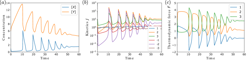
Through a conservative CRN example, we confirm the behaviour of our defined physical quantities. The Brusselator is used for numerical experiment, which is a well-known autocatalytic reaction model showing chemical oscillation [22]. We use the damped version of Brusselator system in [20] which has species and reactions whose reaction equations are represented as
| (50) | |||||
| (51) | |||||
| (52) |
Formally, the reaction set is defined as
| (53) |
where is identified with . The kinetics is assumed to be mass-actional as follows.
| (54) | ||||
| (55) | ||||
| (56) | ||||
| (57) | ||||
| (58) | ||||
| (59) |
where the notation means the concentration of the chemical species . The conventional flux and driving forces are defined as and for . The system exhibits damped oscillations in concentration, kinetics and thermodynamic driving forces in 2.
The S-graph of this system has an edge set
| (60) |
whose reversibility is inherited from the original CRN. The transition for a conservation law has elements with
| (61) | ||||
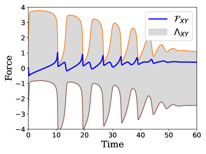
The behaviour of the specieswise force and activity from to and their bounds are observed. As seen in the subsection IV.1, could take values in the interval
| (62) |
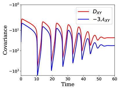
at each time. The time evolutions of and the possible interval are showed in Fig 3. In this simulation, we can comfirm that the area is actually for any time . The force and its upper bound is quite close at certain times, which is interpreted by the asymtotic approximation discussed in the last of the subsection IV.1, together with the time series of the kinetics Fig 2 (b). The time evolutions of the covariance between and the lower bound is seen in the Fig 4. Again, it can be seen that the two physical quantities are approximately coincident in situations where the largest reaction order, reaction 2, is dominant.
By observing the numerical results, two properties can be identified for our defined quantities below. First, we argue that the physical quantities we have defined are properly interpretable. Indeed, we have so far confirmed both theoretically and numerically that specieswise forces and activities are related to conventional driving forces and covariance. In particular, for the former, Figure 2 (a) shows that increases and decreases in the long term, which is consistent with a positive to force for most of the time . Secondly, the specieswise force and activity is found to inherit the oscillatory nature of the system in the simulation.
VI conclusion and discussion
This paper introduced a novel framework for analyzing CRN dynamics by defining ”transitions” as a new physical quantity and reinterpreting the dynamics on a species graph. The dynamics on this graph were proven conservative by scaling concentrations according to the network’s conservation laws. Thermodynamic quantities like forces and activities were then formulated at the species level based on these transitions and the relation between the specieswise thermodynamic quantities and conventional thermodynamic quantities were investigated. When applied numerically to the Brusselator oscillating reaction system, the specieswise quantities exhibited intuitive behavior aligned with theoretical predictions. This transition-based graphical approach provides an alternative perspective for understanding the thermodynamics of complex CRNs with potential for enhanced modeling and analysis. Further research is merited into the broader implications and applications of this specieswise thermodynamic formulation.
One potential limitation of our framework is that the newly introduced concept of ”transitions” may not precisely mirror the actual physical transformations occurring at the molecular level. To illustrate, consider a second-order chemical reaction through which the physical chemistry explains the molecules and undergo structural changes to become and respectively. Following this depiction, the reaction should solely contribute to the transitions and . However, our methodology additionally accounts for the transitions and , which do not directly correspond to the molecular rearrangements. Despite this potential disconnect from microscopic mechanisms, our transition-based approach offers the significant advantage of being systematically computable from the system’s stoichiometric and kinetic information, lending itself to practical analysis workflows.
Looking ahead, we anticipate our framework enabling deeper dynamical analysis of reaction networks, particularly metabolic systemsand others central to cellular processes. Theoretically, exploring how stochastic thermodynamics laws manifest in CRNs under our specieswise formulation is intriguing. For instance, it is an interesting topic that how the relations between correlations and driving forces at a steady state for Markov jump system [23] potentially transform in the CRN context. As this specieswise approach develops, prospects include analyzing complex network dynamics and bridging disparate fields through a unified reaction network lens, with potential for significant discoveries.
References
- Orth et al. [2010] J. Orth, I. Thiele, and B. Palsson, What is flux balance analysis?, Nature biotechnology 28, 245 (2010).
- van Zon et al. [2007] J. S. van Zon, D. K. Lubensky, P. R. H. Altena, and P. R. ten Wolde, An allosteric model of circadian kaic phosphorylation, Proceedings of the National Academy of Sciences 104, 7420 (2007), https://www.pnas.org/doi/pdf/10.1073/pnas.0608665104 .
- Avanzini et al. [2024] F. Avanzini, M. Bilancioni, V. Cavina, S. D. Cengio, M. Esposito, G. Falasco, D. Forastiere, N. Freitas, A. Garilli, P. E. Harunari, V. Lecomte, A. Lazarescu, S. G. M. Srinivas, C. Moslonka, I. Neri, E. Penocchio, W. D. Piñeros, M. Polettini, A. Raghu, P. Raux, K. Sekimoto, and A. Soret, Methods and conversations in (post)modern thermodynamics, SciPost Phys. Lect. Notes , 80 (2024).
- Yoshimura and Ito [2021a] K. Yoshimura and S. Ito, Thermodynamic uncertainty relation and thermodynamic speed limit in deterministic chemical reaction networks, Phys. Rev. Lett. 127, 160601 (2021a).
- Kobayashi et al. [2023] T. J. Kobayashi, D. Loutchko, A. Kamimura, S. A. Horiguchi, and Y. Sughiyama, Information geometry of dynamics on graphs and hypergraphs, Information Geometry 10.1007/s41884-023-00125-w (2023).
- Himeoka et al. [2024] Y. Himeoka, S. A. Horiguchi, and T. J. Kobayashi, Stoichiometric rays: A simple method to compute the controllable set of enzymatic reaction systems (2024), arXiv:2403.02169 [physics.bio-ph] .
- Watts and Strogatz [1998] D. J. Watts and S. H. Strogatz, Collective dynamics of ‘small-world’ networks, Nature 393, 440–442 (1998).
- Newman [2018] M. Newman, Networks (Oxford University Press, 2018).
- Angeli et al. [2009] D. Angeli, P. De Leenheer, and E. Sontag, Graph-theoretic characterizations of monotonicity of chemical networks in reaction coordinates, Journal of Mathematical Biology 61, 581–616 (2009).
- Wagner and Fell [2001] A. Wagner and D. A. Fell, The small world inside large metabolic networks, Proceedings of the Royal Society of London. Series B: Biological Sciences 268, 1803–1810 (2001).
- Klamt et al. [2009] S. Klamt, U.-U. Haus, and F. Theis, Hypergraphs and cellular networks, PLOS Computational Biology 5, 1 (2009).
- Himeoka and Kaneko [2016] Y. Himeoka and K. Kaneko, Enzyme oscillation can enhance the thermodynamic efficiency of cellular metabolism: consequence of anti-phase coupling between reaction flux and affinity, Physical Biology 13, 026002 (2016).
- Kim and Hyeon [2021] P. Kim and C. Hyeon, Thermodynamic optimality of glycolytic oscillations, The Journal of Physical Chemistry B 125, 5740 (2021), pMID: 34038120, https://doi.org/10.1021/acs.jpcb.1c01325 .
- Fontanil and Mendoza [2022] L. Fontanil and E. Mendoza, Common complexes of decompositions and complex balanced equilibria of chemical reaction networks, MATCH Communications in Mathematical and in Computer Chemistry 87, 329 (2022).
- Feinberg [2019] M. Feinberg, Foundations of Chemical Reaction Network Theory (Springer International Publishing, 2019).
- Müller et al. [2022] S. Müller, C. Flamm, and P. F. Stadler, What makes a reaction network ”chemical”?, J Cheminform 14, 63 (2022).
- De Martino et al. [2014] A. De Martino, D. De Martino, R. Mulet, and A. Pagnani, Identifying all moiety conservation laws in genome-scale metabolic networks, PLOS ONE 9, 1 (2014).
- Grady and Polimeni [2010] L. J. Grady and J. R. Polimeni, Discrete Calculus (Springer London, 2010).
- Seifert [2012] U. Seifert, Stochastic thermodynamics, fluctuation theorems and molecular machines, Reports on Progress in Physics 75, 126001 (2012).
- Yoshimura and Ito [2021b] K. Yoshimura and S. Ito, Information geometric inequalities of chemical thermodynamics, Phys. Rev. Res. 3, 013175 (2021b).
- Gillespie [2000] D. T. Gillespie, The chemical Langevin equation, The Journal of Chemical Physics 113, 297 (2000), https://pubs.aip.org/aip/jcp/article-pdf/113/1/297/19042305/297_1_online.pdf .
- Lefever et al. [1988] R. Lefever, G. Nicolis, and P. Borckmans, The brusselator: it does oscillate all the same, Journal of the Chemical Society, Faraday Transactions 1: Physical Chemistry in Condensed Phases 84, 1013 (1988).
- Ohga et al. [2023] N. Ohga, S. Ito, and A. Kolchinsky, Thermodynamic bound on the asymmetry of cross-correlations, Phys. Rev. Lett. 131, 077101 (2023).