Regularized Conformal Electrodynamics: Novel C-metric in (2+1) Dimensions
Abstract
Conformal electrodynamics is a particularly interesting example of power Maxwell non-linear electrodynamics, designed to possess conformal symmetry in all dimensions. In this paper, we propose a regularized version of Conformal electrodynamics, minimally regularizing the field of a point charge at the origin by breaking the conformal invariance of the theory with a dimensionfull ‘Born–Infeld-like’ parameter. In four dimensions the new theory reduces to the recently studied Regularized Maxwell electrodynamics, distinguished by its ‘Maxwell-like’ solutions for accelerated and slowly rotating black hole spacetimes. Focusing on three dimensions, we show that the new theory shares many of the properties of its four-dimensional cousin, including the existence of the charged C-metric solution (currently unknown in the Maxwell theory).
I Introduction
Non-linear electrodynamics (NLE) arose out of attempts to deal with singular nature of classical Maxwell’s (linear) theory of electrodynamics when applied to point charges. One of the first and certainly the most famous non-linear model was proposed by Born and Infeld almost hundred years ago [1] – it is distinguished by absence of birefringence and other unique properties [2]. Subsequently, other models were proposed to achieve better regularization [3], or to embody quantum corrections to Maxwell’s theory coming from QED [4] and (much later) string theory [5]. More recently, NLE was used as a ‘physical’ source of regular black holes [6], increasing its significance for ‘physics of spacetime’. In this regard, one may formulate new criterion for importance of a given NLE model by demanding its compatibility with essential spacetime geometries (going beyond spherical symmetry) [7, 8, 9, 10], thus mimicking the success of Maxwell’s linear theory in this regard.
While predominantly studied in four dimensions, theories of nonlinear electrodynamics are also interesting in lower/higher-dimensional settings. Among these, Conformal electrodynamics [11] is of particular interest. It is a special example of power Maxwell electrodynamics [12], designed in a way to preserve Weyl symmetry in any number of dimensions, such that in four dimensions it reduces to the Maxwell theory and yields dimension-independent (four-dimensional) Coulomb law for a point charge.
In this paper, we propose a regularized version of Conformal electrodynamics. Namely, we design a 1-parametric generalization of Conformal electrodynamics characterized by a dimensionalfull Born–Infeld-like parameter , which yields a finite (minimally regularized) field of a point charge in the origin. While the new Regularized Conformal electrodynamics naturally breaks the Weyl symmetry of the original theory, it possesses a number of interesting properties. Namely, in four dimensions it reduces to the recently studied Regularized Maxwell (RegMax) electrodynamics, which is a unique NLE (constructed from a single field invariant that admits ‘Maxwell-like’ Robinson–Trautman [7, 10], C-metric [9], and slowly-rotating [8] spacetimes (see also [13] for a recent discussion of optical properties of the corresponding RegMax black holes). As we shall show in this paper, in three dimensions the regularized theory admits a well behaved generalized charged BTZ black hole with improved thermodynamic charges that are not ‘plagued’ by at infinity logarithmically divergent vector potential. Perhaps most importantly, it also admits a novel charged C-metric solution (at the moment unknown to exist in 3-dimensional Einstein–Maxwell theory). We shall argue that the last property is very exceptional among all 3-dimensional theories of NLE.
Our paper is organized as follows. The basic properties of NLE theories are reviewed in the next section. Conformal electrodynamics together with an overview of its spherical solutions are gathered in Sec. III. The novel Regularized Conformal electrodynamics is proposed in Sec. IV. Focusing on three dimensions, the corresponding generalized charged BTZ black holes solutions are studied in Sec. V. The novel charged C-metric in dimensions is constructed in Sec. VI. We conclude in Sec. VII. Appendix A overviews spherical charged black holes in the Maxwell theory, while Appendix B is devoted to construction of rotating charged BTZ black holes.
II Theories of nonlinear electrodynamics
In this paper we consider Einstein gravity coupled to non-linear electrodynamics, described by the following -dimensional action:
| (1) |
allowing for a possibility of (negative) cosmological constant , which we parameterize in terms of the corresponding AdS radius as follows:
| (2) |
and relate it to the thermodynamic pressure according to, e.g. [14]:
| (3) |
Here, is the electromagnetic Lagrangian, which is taken to be a function of electromagnetic field strength invariants of the Maxwell tensor (not considering its covariant derivatives). In number of spacetimes dimensions, there are up to such invariants, related to the non-trivial eigenvalues of . One convenient way for extracting such eigenvalues is for example to consider the traces of the even powers of the Maxwell tensor, namely
| (4) |
see e.g. [15] for a construction of quasitopological electromagnetism in terms of powers of such traces.
A canonical example of non-linear electrodynamics is the Born-Infeld theory [1], whose Lagrangian in all dimensions is naturally written as (see e.g. [16] for examples of solutions in higher dimensions):
| (5) |
where is the Born–Infeld dimensionfull parameter (with dimensions ), which regularizes the field of a point charge and determines the maximal field strength allowed in the theory. Theories considered in this paper will possess similar parameter.
In this paper we focus on a ‘simple’ class of non-linear theories that are characterized by a single electromagnetic invariant:111In spacetime dimensions (of main interest in this paper) this is really no restriction, as any NLE therein is characterized by a single field invariant.
| (6) |
To further restrict the possibilities, one might require that a given theory of non-linear electrodynamics should approach that of Maxwell in the weak field approximation:
| (7) |
a condition known as the principle of correspondence. However, while such a condition is important in four dimensions, there is no reason a priori to consider it in other dimensions as well. In particular, theories studied in this paper will obey the principle of correspondence in four dimensions but will not approach Maxwell’s theory in other dimensions.222Another criterion for restricting possible non-linear theories of electrodynamics is related to the birefringence phenomena, causality, and energy conditions. In this work we shall not deal with these issues and refer the interested reader to recent papers on this topic [17, 18, 19].
Introducing the following notation:
| (8) |
the generalized Maxwell equations read
| (9) |
where
| (10) |
We also obtain the following Einstein equations:
| (11) |
where the generalized EM energy-momentum tensor reads
| (12) |
We shall discuss various examples of non-linear electrodynamics below.
III Conformal electrodynamics
The conformal electrodynamics [11] is described by the following Lagrangian:
| (13) |
where is a dimensionfull coupling constant, with dimensions . Obviously, in this reduces to the Maxwell electrodynamics (7). Moreover, upon the Weyl scaling and , we find that remains in any number of dimensions invariant. We also have
| (14) |
With this it is easy to check that the corresponding energy-momentum tensor (12) is traceless, .
III.1 Spherical solutions
In any number of spacetime dimensions, the field of a point charge in conformal electrodynamics is given by the (four-dimensional) Coulomb law:
| (15) |
where is a charge parameter of dimensions of length; in what follows (and to simplify our notations) we restrict ourselves to positive charges, . Then, is related to the electric charge according to the following formula:
| (16) |
where is the volume of the -dimensional sphere, namely
| (17) |
The corresponding spherically symmetric solution is then given by [20, 21] (see Appendix A for comparison to solutions in standard Einstein–Maxwell theory):
| (18) |
where stands for the standard element on , and the metric function reads
| (19) |
One can show that when the above solution describes a black hole, the corresponding thermodynamic quantities are given by (see also [22, 23]):
| (20) |
With these at hand, it is easy to verify that the following extended first law holds:
| (21) |
which reduces to the standard first law upon fixing the cosmological constant and the coupling constant . The above first law is accompanied by the corresponding extended Smarr relation, which reads
| (22) |
with the two related by Euler’s scaling argument.
III.2 Conformally charged BTZ black hole
Contrary to Maxwell’s case (see Appendix A), many of the above formulae remain also valid in dimensions. Let us state these explicitly for future reference. Namely, in , the conformal electrodynamics reduces to
| (23) |
and admits the following charged BTZ black hole solution [24, 25, 26]:
| (24) |
where the metric function reads
| (25) |
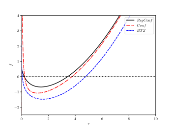
It demonstrates a typical ‘Reissner–Nordström-AdS’-like behavior with two, one extremal, or no black hole horizons. In particular, in Fig. 1 we display and example of a black hole with two horizons and compare it to other charged BTZ black holes studied in this paper.
The solution is characterized by the following thermodynamic charges:
| (26) |
Note that contrary to what happens in Maxwell’s electrodynamics, c.f. (A), thermodynamic volume here is the ‘standard’ 2d geometric volume. One can then easily verify that the above thermodynamic quantities obey the generalized first law (21) and the Smarr formula (22), which now reduces to a simple relation:
| (27) |
without explicit and terms.
IV Regularized conformal electrodynamics
IV.1 Constructing the theory
Let us now construct a theory which minimally regularizes the conformal electrodynamics. More precisely, we seek a theory whose vector potential of a pointlike charge in flat space (written in spherical coordinates) takes the following minimally regularized form in any number of dimensions:
| (28) |
Here we have introduced a dimensionfull ‘Born–Infeld-like’ parameter , which plays the role of a ‘maximum field strength’ and has dimensions ; the conformal electrodynamics is recovered upon setting
| (29) |
Calculating the field invariant for the above field, we find
| (30) |
The generalized Maxwell equation (9) in dimensions then reads
| (31) |
Upon integrating this equation and expressing in terms of via (30), we recover
| (32) |
where is some (rescaled) integration constant, and we introduced a shorthand
| (33) |
Expanding (32) for large and comparing it to (14), fixes the integration constant to , giving
| (34) |
The full Lagrangian is then obtained by integration:
| (35) |
This yields the following Regularized Conformal (RegConf) theory:
| (36) |
where the integration constant needs to be fixed so that we recover the conformal electrodynamics in the large limit.
IV.2 Three dimensions
In what follows we shall focus on the regularized conformal electrodynamics in dimensions. Let us summarize here the corresponding formulae. The theory is described by the following Lagrangian:
| (38) |
In addition to the dimensionfull parameter of the conformal electrodynamics, the theory is characterized by a new dimensionfull parameter , , and reduces to the conformal electrodynamics in dimension upon setting
| (39) |
Namely, we have
| (40) |
the limit yields the vacuum case. The first and second derivatives of with respect to , that are important for the field equations and the optical metric, are given by
| (41) |
We shall now turn to constructing simple (black hole) solutions in this theory.
V Generalized charged BTZ black hole
Let us first show that the Regularized Conformal electrodynamics in dimensions admits a charged BTZ-like black hole solution, generalizing (III.2). It takes the following simple form:
| (42) | |||||
| (43) |
where the metric function reads
| (44) | |||||
The corresponding field strength
| (45) |
approaches a finite value in the origin, . For large (or alternatively large ) we recover the conformal electrodynamics metric function:
| (46) |
On the other hand, near the origin, , we find
| (47) |
Although the metric function remains finite at the origin, the black hole solution possesses a singularity at , as can for example be seen by expanding the Ricci scalar. In particular, setting for the moment, we find the following expansions for the Ricci and Kretschmann scalars:
| (48) |
This is to be compared to the vanishing Ricci scalar of the conformal BTZ black hole (III.2), as well as to its (significantly more divergent) Kretschmann scalar, .
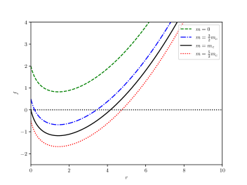
In order to have a black hole, we have to have . Dependent on the choice of parameters we then obtain three ‘types’ of black holes, see Fig. 2. Namely, since at the metric function remains finite:
| (49) |
if , we have the ‘Reissner–Nordström’ branch, with timelike singularity and two, one extremal, or no black hole horizons. If , we have the ‘Schwarzschild’ branch with spacelike singularity and one black hole horizon. Finally, is the marginal case, characterized by . Formally, the origin becomes a ‘horizon’, though the curvature scalars still diverge there. At the same time this ‘place’ is point-like since we use the ‘area gauge’ for the coordinate . This behavior is similar to what happens in the scalar field spacetimes in four-dimensional general relativity [27], where a notion of the so-called ‘black point’ is used for its description. This type of ‘null point-like singularity’ prevails also for scalar field spacetimes in the presence of non-linear electrodynamics [28].
The above generalized BTZ black hole can be assigned the following thermodynamic quantities:
| (50) |
together with
| (51) | |||||
It is easy to verify that these obey the following extended first law:
| (52) |
together with the corresponding Smarr relation:
| (53) |
Unfortunately, contrary to their four-dimensional cousins, the 3-dimensional RegConf black holes do not seem to admit any remarkable thermodynamic behavior.
VI Novel charged C-metric in (2+1) dimensions
Recently there has been a lot of interest in 3-dimensional C-metric [32, 33], see e.g. [34, 35] for analysis of the solution and [36, 37, 38] for attempts at its thermodynamic interpretation. Since its first discovery, the vacuum solution [32, 33] has been generalized to include scalar field [39] and most recently also to conformal electrodynamics [40]. While the solution may not exist in Maxwell’s theory (see below), in this section we generalize it to the Regularized Conformal electrodynamics.
VI.1 Accelerated BTZ black hole
The -dimensional vacuum C-metric is most easily written in the so called ‘’ coordinates [32, 33, 34], and reads
| (54) |
where the conformal factor is
| (55) |
with an acceleration parameter (of dimensions of ), and the metric functions and that take the following form:
| (56) |
Such a metric can describe accelerated particle-like solutions or black holes. Focusing on accelerated black holes that are smoothly connected to a BTZ black hole, we set
| (57) |
upon which
| (58) |
and (to preserve the signature of the spacetime) we have to have (or alternatively ). More concretely, let be the appropriate range of coordinate , with . The zeroes of the metric function determine the position of the black hole () and Rindler () horizons; explicitly these are given by
| (59) |
We can now distinguish two cases: i) the case of rapid acceleration, which happens for , and in which case both horizons are present and ii) the case of slowly accelerating black holes with no Rindler horizon, for which .
To make connections with the 4-dimensional C-metric, e.g. [41, 42], let us perform the following change of coordinates [34]:
| (60) |
upon which the metric takes a ‘more familiar form’:
| (61) |
where
| (62) |
Here, regulates the tension of the wall pulling the black hole and ensures that , and is not an independent parameter, but rather a combination of other parameters, ensuring the proper normalization of the proper time of an asymptotic observer.
We shall not attempt to review more properties of the above solution here and refer the interested reader to the original literature above. Instead, we proceed directly to finding the corresponding charged generalization in Regularized Conformal electrodynamics.
VI.2 Regularized charged C-metric
To find the charged generalization of the above vacuum solution in Regularized Conformal electrodynamics, we employ the ansatz (54) and (55), and accompany it with the following ansatz for the vector potential:
| (63) |
The Einstein equations together with the generalized Maxwell equation then yield the following solution:
| (64) |
and
| (65) |
The solution looks remarkably similar to its four-dimensional cousin in this theory, c.f. Sec. V.A in [9]. In particular, note that when the cosmological constant vanishes, the functions and have the following property: . Similar to the vacuum case, to maintain a Lorentzian signature of the metric (54), it is necessary that , which implies restrictions on the domain of coordinate . We postpone the detailed discussion of this solution to a future study. Here we only make two remarks.
First, in the large limit we recover the charged C-metric in conformal electrodynamics studied in [40], namely:
| (66) |
together with
| (67) |
Second, one can easily check that while we were able to construct the charged C-metric for the conformal electrodynamics and its regularized generalization, the ansatz (54) together with (63) are incompatible with many other theories of NLE, including the Maxwell theory. Namely, starting with any NLE, and using the ansatz (63), the time component of the modified Maxwell equation, , can be once integrated, to yield
| (68) |
where is an integration ‘constant’, a function of -coordinate only. However, since the corresponding obeys , we must also have , that is, has to be separable:
| (69) |
Moreover, for the spacetime to describe the C-metric, as we know it, both such parts have to be non-trivial. Thus the previous equation (68) imposes a very strict restriction on the form of for a given theory, namely
| (70) |
for some function . Obviously, for Maxwell, and the previous equation cannot be satisfied. Remarkably, for the Regularized C-metric solution above, we find
| (71) |
which is precisely of the form above. It remains to be seen, whether the Regularized Conformal electrodynamics is the most general theory for which the equation (70) can be satisfied.
VII Summary
Conformal electrodynamics is a very interesting example of a power Maxwell theory characterized by preserving the Weyl symmetry in any number of dimensions. In four dimensions it coincides with the Maxwell theory, while it breaks the principle of correspondence in any other dimension.
In this paper we have generalized the recently studied four-dimensional RegMax electrodynamics to any number of dimensions. A foundational feature of the new theory (inherited from its four-dimensional cousin) is that it minimally regularizes the field of a point charge – it is characterized by a dimensionfull Born–Infeld-like parameter, which imposes a maximal bound on the field strength at the position of the charge. In addition, we have designed our theory so that in any number of dimensions it reduces to the Conformal electrodynamics (and in particular to the Maxwell theory in four dimensions) in the weak field limit – thence the name Regularized Conformal electrodynamics.
Moreover, focusing on three dimensions, we have shown that the new theory admits charged BTZ-like black holes with vanishing at infinity vector potential, giving rise to a much simpler thermodynamic interpretation than is the case of the Maxwell charged BTZ black holes whose potential logarithmically diverges at infinity. Even more remarkably, the theory admits a 3-dimensional generalization of a charged C-metric, thus providing a non-trivial example of charged accelerating black holes in three dimensions, a property it shares with its four-dimensional RegMax cousin. We suspect that Regularized Conformal electrodynamics may be the most general theory for which the accelerated charged black holes can be found in the above studied form.
The extension of the RegMax theory beyond four dimensions is of course not unique. For example, instead of demanding that the theory in the weak field limit approaches that of the Conformal electrodynamics, we might have required it to approach the Maxwell electrodynamics instead, giving rise to ‘genuine’ RegMax electrodynamics in all dimensions. Namely, instead of the potential (28) we could have demanded that it goes like:
| (72) |
c.f. Eq. (A) in Appendix A(or, in dimensions instead of (A). However, the corresponding theory does not seem to give raise to C-metric solutions in three dimensions. It may, however, be interesting in higher dimensions, for example in connection with slowly rotating black holes. We leave this endeavor for future studies.
Acknowledgements
D.K. and T.T. are grateful for support from GAČR 23-07457S grant of the Czech Science Foundation. O.S. is supported by Research Grant No. GAČR 22-14791S. D.K. acknowledges the Charles University Research Center Grant No. UNCE24/SCI/016.
Appendix A Charged black hole in Maxwell theory
The charged AdS black holes in Maxwell theory in number of spacetime dimensions take the following standard form, e.g. [43]:
| (73) |
where stands for the standard element on , and the metric function reads
| (74) |
Here, the electric charge is given by
| (75) |
and the mass reads
| (76) |
The remaining thermodynamic quantities are
| (77) |
Together, they obey the standard first law of thermodynamics:
| (78) |
The above solution is valid in dimensions. For , one has instead the charged BTZ black hole [44, 45]. It reads as follows:
| (79) |
where
| (80) |
Here, is a dimensionfull constant with dimensions of length; often in the literature is simply associated with the AdS length scale, , e.g. [46]. The logarithmic divergence renders calculation of the asymptotic mass a bit problematic, see, e.g. [47] for a a possible renormalization procedure. In any case, the solution can be assigned the following thermodynamic quantities [46]:
| (81) |
note the departure of from the ‘standard geometric volume’. In any case, the above thermodynamic quantities obey the above standard first law (78).
Appendix B Rotating charged BTZ black holes
Rotating charged BTZ-like black holes (in any NLE) can be obtained from non-rotating ones by the following trick [30, 31]. Start from a static solution
| (82) |
and apply the following boost:
| (83) |
This, upon the right identification of the new coordinate , yields the rotating and charged BTZ-like black hole solution
| (84) |
where
| (85) |
References
- [1] M. Born and L. Infeld, Foundations of the new field theory, Proc. Roy. Soc. Lond. A 144 (1934) 425.
- [2] J. Plebański, Lectures on non-linear electrodynamics: an extended version of lectures given at the Niels Bohr Institute and NORDITA, Copenhagen, in October 1968, vol. 25, Nordita (1970).
- [3] B. Hoffmann and L. Infeld, On the choice of the action function in the new field theory, Phys. Rev. 51 (1937) 765.
- [4] W. Heisenberg and H. Euler, Consequences of Dirac’s theory of positrons, Z. Phys. 98 (1936) 714 [physics/0605038].
- [5] E.S. Fradkin and A.A. Tseytlin, Nonlinear Electrodynamics from Quantized Strings, Phys. Lett. B 163 (1985) 123.
- [6] E. Ayon-Beato and A. Garcia, Regular black hole in general relativity coupled to nonlinear electrodynamics, Phys. Rev. Lett. 80 (1998) 5056 [gr-qc/9911046].
- [7] T. Tahamtan, Compatibility of nonlinear electrodynamics models with Robinson-Trautman geometry, Phys. Rev. D 103 (2021) 064052 [2010.01689].
- [8] D. Kubiznak, T. Tahamtan and O. Svitek, Slowly rotating black holes in nonlinear electrodynamics, Phys. Rev. D 105 (2022) 104064 [2203.01919].
- [9] T. Hale, D. Kubizňák, O. Svítek and T. Tahamtan, Solutions and basic properties of regularized Maxwell theory, Phys. Rev. D 107 (2023) 124031 [2303.16928].
- [10] T. Tahamtan, D. Flores-Alfonso and O. Svitek, Well-posed nonvacuum solutions in Robinson-Trautman geometry, Phys. Rev. D 108 (2023) 124076 [2311.03110].
- [11] M. Hassaïne and C. Martínez, Higher-dimensional black holes with a conformally invariant maxwell source, Phys. Rev. D 75 (2007) 027502.
- [12] M. Hassaïne and C. Martínez, Higher-dimensional charged black hole solutions with a nonlinear electrodynamics source, Classical and Quantum Gravity 25 (2008) 195023.
- [13] T. Hale, D. Kubiznak and J. Menšíková, Optical properties of black holes in regularized Maxwell theory, 2401.16259.
- [14] D. Kubiznak, R.B. Mann and M. Teo, Black hole chemistry: thermodynamics with Lambda, Class. Quant. Grav. 34 (2017) 063001 [1608.06147].
- [15] H.-S. Liu, Z.-F. Mai, Y.-Z. Li and H. Lü, Quasi-topological Electromagnetism: Dark Energy, Dyonic Black Holes, Stable Photon Spheres and Hidden Electromagnetic Duality, Sci. China Phys. Mech. Astron. 63 (2020) 240411 [1907.10876].
- [16] S. Li, H. Lu and H. Wei, Dyonic (A)dS Black Holes in Einstein-Born-Infeld Theory in Diverse Dimensions, JHEP 07 (2016) 004 [1606.02733].
- [17] J.G. Russo and P.K. Townsend, Nonlinear electrodynamics without birefringence, JHEP 01 (2023) 039 [2211.10689].
- [18] J.G. Russo and P.K. Townsend, On Causal Self-Dual Electrodynamics, 2401.06707.
- [19] J.G. Russo and P.K. Townsend, Causality and Energy Conditions in Nonlinear Electrodynamics, 2404.09994.
- [20] M. Hassaine and C. Martinez, Higher-dimensional black holes with a conformally invariant Maxwell source, Phys. Rev. D 75 (2007) 027502 [hep-th/0701058].
- [21] M. Hassaine and C. Martinez, Higher-dimensional charged black holes solutions with a nonlinear electrodynamics source, Class. Quant. Grav. 25 (2008) 195023 [0803.2946].
- [22] H.A. Gonzalez, M. Hassaine and C. Martinez, Thermodynamics of charged black holes with a nonlinear electrodynamics source, Phys. Rev. D 80 (2009) 104008 [0909.1365].
- [23] S.H. Hendi and M.H. Vahidinia, Extended phase space thermodynamics and P-V criticality of black holes with a nonlinear source, Phys. Rev. D 88 (2013) 084045 [1212.6128].
- [24] M. Cataldo, N. Cruz, S. del Campo and A. Garcia, (2+1)-dimensional black hole with Coulomb - like field, Phys. Lett. B 484 (2000) 154 [hep-th/0008138].
- [25] O. Gurtug, S.H. Mazharimousavi and M. Halilsoy, 2+1-dimensional electrically charged black holes in Einstein - power Maxwell Theory, Phys. Rev. D 85 (2012) 104004 [1010.2340].
- [26] M. Cataldo, P.A. González, J. Saavedra, Y. Vásquez and B. Wang, Thermodynamics of ( 2+1 )-dimensional Coulomb-like black holes from nonlinear electrodynamics with a traceless energy momentum tensor, Phys. Rev. D 103 (2021) 024047 [2010.06089].
- [27] J. Winicour, A.I. Janis and E.T. Newman, Static, Axially Symmetric Point Horizons, Phys. Rev. 176 (1968) 1507.
- [28] T. Tahamtan, Scalar hairy black holes in the presence of nonlinear electrodynamics, Phys. Rev. D 101 (2020) 124023 [2006.02810].
- [29] G. Clement, Classical solutions in three-dimensional Einstein-Maxwell cosmological gravity, Class. Quant. Grav. 10 (1993) L49.
- [30] G. Clement, Spinning charged BTZ black holes and selfdual particle - like solutions, Phys. Lett. B 367 (1996) 70 [gr-qc/9510025].
- [31] C. Martínez, C. Teitelboim and J. Zanelli, Charged rotating black hole in three spacetime dimensions, Phys. Rev. D 61 (2000) 104013.
- [32] M. Astorino, Accelerating black hole in 2+1 dimensions and 3+1 black (st)ring, JHEP 01 (2011) 114 [1101.2616].
- [33] W. Xu, K. Meng and L. Zhao, Accelerating BTZ spacetime, Class. Quant. Grav. 29 (2012) 155005 [1111.0730].
- [34] G. Arenas-Henriquez, R. Gregory and A. Scoins, On acceleration in three dimensions, JHEP 05 (2022) 063 [2202.08823].
- [35] R.D.B. Fontana and A. Rincon, Accelerated black holes in (2+1) dimensions: Quasinormal modes and Stability, 2404.09936.
- [36] G. Arenas-Henriquez, A. Cisterna, F. Diaz and R. Gregory, Accelerating Black Holes in dimensions: Holography revisited, JHEP 09 (2023) 122 [2308.00613].
- [37] J. Tian and T. Lai, Aspects of three-dimensional C-metric, JHEP 03 (2024) 079 [2401.04457].
- [38] J. Tian and T. Lai, Thermodynamics and Holography of Three-dimensional Accelerating black holes, 2312.13718.
- [39] A. Cisterna, F. Diaz, R.B. Mann and J. Oliva, Exploring accelerating hairy black holes in 2+1 dimensions: the asymptotically locally anti-de Sitter class and its holography, JHEP 11 (2023) 073 [2309.05559].
- [40] B. Eslam Panah, Charged Accelerating BTZ Black Holes, Fortsch. Phys. 71 (2023) 2300012 [2203.12619].
- [41] A. Anabalón, M. Appels, R. Gregory, D. Kubizňák, R.B. Mann and A. Ovgün, Holographic Thermodynamics of Accelerating Black Holes, Phys. Rev. D 98 (2018) 104038 [1805.02687].
- [42] A. Anabalón, F. Gray, R. Gregory, D. Kubizňák and R.B. Mann, Thermodynamics of Charged, Rotating, and Accelerating Black Holes, JHEP 04 (2019) 096 [1811.04936].
- [43] S. Gunasekaran, R.B. Mann and D. Kubiznak, Extended phase space thermodynamics for charged and rotating black holes and Born-Infeld vacuum polarization, JHEP 11 (2012) 110 [1208.6251].
- [44] M. Bañados, C. Teitelboim and J. Zanelli, Black hole in three-dimensional spacetime, Phys. Rev. Lett. 69 (1992) 1849.
- [45] M. Bañados, M. Henneaux, C. Teitelboim and J. Zanelli, Geometry of the 2+1 black hole, Phys. Rev. D 48 (1993) 1506.
- [46] A.M. Frassino, R.B. Mann and J.R. Mureika, Lower-Dimensional Black Hole Chemistry, Phys. Rev. D 92 (2015) 124069 [1509.05481].
- [47] M. Cadoni, M. Melis and M.R. Setare, Microscopic entropy of the charged BTZ black hole, Class. Quant. Grav. 25 (2008) 195022 [0710.3009].