Change-point analysis for binomial autoregressive model with application to price stability counts

1 Introduction

In recent years, modeling and analysis of count time series have become an attractive issue with a large quantity of articles in fields like epidemiology, social sciences, economics, life sciences and others. One of the most commonly used approaches to analyze count time series is to construct integer-valued time series models based on different types of thinning operators. In particular, the binomial thinning operator is the most popular one in real-world applications since its simplicity and high interpretability. The binomial thinning operator, which was proposed by Steutel and Van Harn (1979), is defined as

$$\alpha\circ X=\sum_{i=1}^{X}B_{i},$$

where $\alpha\in(0,1)$, $\{B_{i}\}$ is an independent and identically distributed (i.i.d.) Bernoulli($\alpha$) random sequence independent of non-negative integer-valued random variable $X$.

Based on the different actual background, the research on count time series is mainly divided into statistical inference for unbounded and bounded integer-valued time series model. On one hand, the unbounded count time series (having a range contained in $\mathbb{N}_{0}=\{0,1,2,...\}$) are frequently encountered in practice, such as monthly unemployment figures, counts of fatal accidents, severe injury accidents, minor injury accidents, vehicle damage accidents and so on. First-order integer-valued autoregressive (INAR(1)) model based on the binomial thinning operator is the most commonly applied tool to deal with the unbounded count time series. We give the definition of the INAR(1) model as follows.

Definition 1

The INAR(1) model $\{X_{t}\}_{t\geqslant 1}$ is defined by the following recursion

$$X_{t}=\alpha\circ X_{t-1}+\epsilon_{t},~{}t=1,2,...,$$

where $``\circ"$ is the binomial thinning operator, $\{\epsilon_{t}\}$ is a sequence of i.i.d. integer-valued random variables and $\epsilon_{t}$ is not depending on past values of $\{X_{s}\}_{s<t}$.

Due to the flexibility and practicability of the INAR(1) model, a large quantity of articles focusing on the modeling and statistical inference for the INAR(1) model have arisen. For example, Al-Osh and Alzaid (1987), Scotto et al. (2018), Barreto-Souza (2019), Darolles et al. (2019), Kang et al. (2020b, 2022, 2023) and Rao et al. (2022) considered the modeling of the INAR(1) models to better handle the fitting problems for unbounded count time series. Pedeli et al. (2015), Jentsch and Wei$\ss$ (2019) studied the parameter estimation for the INAR(1) models. McCabe et al. (2011), Lu (2021), Freeland and McCabe (2004b), Maiti and Biswas (2017) detailedly investigated the prediction approaches for the INAR(1) models. Schweer and Wei$\ss$ (2014), Wei$\ss$ et al. (2019) handled the testing problems for overdispersion and zero inflation in INAR(1) models framework. Fernández-Fontelo et al. (2016, 2021), Henderson and Rathouz (2018), Guan and Hu (2022) and Gourieroux and Jasiak (2004) applied the INAR(1) models to under-reported data, longitudinal data and insurance actuarial.

On the other hand, the bounded count time series (with a fixed finite range $\{0,1,2,...,n\}$) are also sometimes suffered, such as the monitoring of computer pools (with $n$ workstations), infections (with $n$ individuals), metapopulations (with $n$ patches) and transactions in the stock market (with $n$ listed companies). The first-order binomial autoregressive (BAR(1)) model, proposed by McKenzie (1985), is the most natural choice to handle this kind of data. We give the definition of the BAR(1) model below.

Definition 2

The BAR(1) process $\{X_{t}\}_{t\geqslant 1}$ is defined by the recursion

$$X_{t}=\alpha\circ X_{t-1}+\beta\circ(N-X_{t-1}),~{}X_{0}\sim\mathrm{B}(N,p),$$ (1.1)

where $``\circ"$ is the binomial thinning operator and $N\in\mathbb{N}$ is a known upper bound of the model, $\beta:=p(1-\rho)$, $\alpha:=\beta+\rho$, $p\in(0,1)$, $\rho\in\displaystyle\left(\max{\left\{-\frac{p}{1-p},-\frac{1-p}{p}\right\}},1\right)$. $\bm{\theta}:=(p,\rho)^{\top}$ is the parameter vector corresponding to the BAR(1) process. The condition mean and variance of the BAR(1) model are ${\rm E}(X_{t}|\mathcal{F}_{t-1})=\rho X_{t-1}+Np(1-\rho)$ and ${\rm Var}(X_{t}|\mathcal{F}_{t-1})=\rho(1-\rho)(1-2p)X_{t-1}+Np(1-\rho)[1-p(1-\rho)]$, respectively, where $\mathcal{F}_{t-1}$ is the $\sigma$-field generated by the whole information up to time $t-1$. All thinnings are performed independently of each other, and the thinnings at time $t$ are independent of $\{X_{s}\}_{s<t}$.

The BAR(1) model is a strictly stationary and ergodic Markov chain with $h$-step transition probabilities (Wei$\ss$ and Pollett, 2012)

$$\mathrm{P}(X_{t}=j|X_{t-h}=i) =\sum_{k=\max\{0,i+j-N\}}^{\min\{i,j\}}\binom{i}{k}\binom{N-i}{j-k}\alpha_{h}^{k}(1-\alpha_{h})^{i-k}\beta_{h}^{j-k}(1-\beta_{h})^{N-i-j+k},$$ (1.2)

where $\beta_{h}=p(1-\rho^{h})$ and $\alpha_{h}=\beta_{h}+\rho^{h}$. During the past ten years, the interest in the BAR(1) process has significantly increased and research on this model has gained plentiful and substantial harvest. For example, Scotto et al. (2014), Wei$\ss$ and Pollett (2014) and Kang et al. (2020b, 2021, 2023, 2024) proposed several extensions to the classical BAR(1) model. Wei$\ss$ and Kim (2013a, b) studied the parameter estimation for the BAR(1) model. Kim and Wei${\ss}$ (2015) and Kim et al. (2018) considered the testing problems for zero inflation and goodness-of-fit in BAR(1) model framework. Wei$\ss$ and Pollett (2012) and Gouveia et al. (2018) applied the BAR(1) model to the ecology, epidemiology and meteorology.

The analysis of change-points, or structural breaks, was initially developed by Page (1954, 1955) for the detection of change in the mean of independent normal observations. In the change-points analysis framework, inferential problems primarily involve two aspects, which are respectively detection and estimation. As for change-points detection, one tests the null hypothesis of no change in the parameters of the statistical model against the alternative hypothesis that parameters of the model change subsequent to at least one unknown change-points. With regard to change-point estimation, researchers are not only interested in the number of change-points, but also attach importance to obtain the location of the change-points. As the continuous improvement of relevant theories, researchers have come to realize that it appears to be of significant importance to incorporate dependent observations into the change-points analysis since the non-stationary time series, which indicated piecewise stationary characteristic, were frequently encountered. During the past few decades, the time series change-points analysis has been vigorously developed and we refer to the studies of Aue and Horváth (2013), Jandhyala et al. (2013) and Aminikhanghahi and Cook (2017) for a general review. Especially, relevant achievements in count time series gradually become abundant and articles concentrating on the change-points analysis for the INAR(1) models frequently arise in recent years. For example, Pap and Szabó (2013) proposed sever test statistics to detect the change-points in the INAR(1) model. Kang and Lee (2009), Yu and Kim (2020) and Lee and Jo (2023) considered the problem of testing for a parameter change in different types of INAR(1) models by taking advantage of the CUSUM test. Kashikar et al. (2013) developed the Poisson INAR($p$) process with change-points and applied it to the two biometrical data sets. Chattopadhyay et al. (2021) considered the problem of change-point analysis for the INAR(1) model with time-varying covariates. Yu et al. (2022) applied the empirical likelihood ratio (ELR) test to uncover a structural change in INAR processes, Sheng and Wang (2024) studied the change-points analysis of the MCP-GCINAR model based on the MDL principle, and optimized by genetic algorithm (GA). For a review of the change-points analysis in count time series, we refer to the survey by Lee and Kim (2021).

However, to our best knowledge, the change-points analysis for time series of counts is mainly considered in unbounded count data. The related research is rare in bounded count data context, although the development would be extremely important for practice. Up to now, there is only one article that studied the relevant issue. Zhang (2023) proposed a BAR(1) model with one change-point and further studied the change-point detection and estimation problems. However, it is well-known that the multiple change-points model is an extension to the one change-point model. Moreover, a significant limitation of one change-point model is that the multiple change-points situation is more commonly observed in practice. Based on the above consideration, we conclude that it is a vitally necessary and significant issue to come up with a solution to modeling the bounded count time series with multiple change-points. To further illustrate the above statement, we consider the following example.

Example 1

Wei$\ss$ and Kim (2014) studied the data set representing how many of the seventeen European Union countries have a monthly inflation rate below 2$\%$ from January 2000 to December 2011. The data set has a range in $\{0,1,2,...,17\}$ and the length of data is 132. Figure 1 shows the time series plot, autocorrelation function (ACF), and partial ACF (PACF). As pointed out by Wei$\ss$ and Kim (2014), they only analyzed the first 84 observations, i.e., the data corresponds to the period 2000-2006, since these data give no reason to doubt a stationarity based on the time series plot. The authors also agreed with the opinion that the stationarity of the series is violated due to the occurrence of economic events since 2007 such as sub-prime crisis and so on. Moreover, based on the sample path in Figure 1, it is not difficult to speculate that a bounded count time series model with multiple change-points is a reasonable choice to analyze this data set.

To achieve the goal of better fitting the non-stationary bounded count time series, this article concentrates on the statistical analysis for the BAR(1) model with multiple change-points. For this, we initially give the definition of the BAR(1) model with multiple change-points and study the statistical inference for the proposed model. Furthermore, the CUSUM test based on the conditional least squares and modified quasi-likelihood estimators are used to detect the change-points. The estimation problems for the number and location of change-points are also handled by utilizing the minimum description length principle. The number and location of change-points are implicitly defined as the optimizer of an objective function, and the searching algorithm based on genetic algorithm is proposed to solve this difficult optimization problem.

The rest contents of this article are organized as follows. In Section 2, the CUSUM test based on the conditional least squares and modified quasi-likelihood estimators is employed to detect the change-points in the BAR(1) model. In Section 3, the definition of the BAR(1) model with multiple change-points is proposed. Furthermore, we utilize the minimum description length criterion to determine the number and locations of the change-points. Section 4 evaluates the proposed test statistics and estimation methods via some simulation studies. In Section 5, to show the usefulness of our model and methods, we apply the proposed model to the monthly price stability counts. The article ends with a conclusion section and all proofs are given in Appendix.

2 CUSUM test for change-point detection

In this section, we focus on the change-point detection in the BAR(1) model. The CUSUM test based on conditional least squares (CLS), modified quasi-likelihood (MQL), and conditional maximum likelihood (CML) estimators are employed. To task it, we set up the null and alternative hypotheses as follows:

$$\mathcal{H}_{0} \rho p X_{1},...,X_{n} \mathcal{H}_{1} \mathcal{H}_{0}$$: and do not change over v.s. : not .

Under $\mathcal{H}_{0}$, we denote the parameter vector by $\bm{\theta}=(\rho,p)^{\top}$, the parameter space by

$$\Theta_{\text{c}}=[\delta,1-\delta]\times\displaystyle\left[\max{\left\{-\frac{p}{1-p},-\frac{1-p}{p}\right\}}+\delta,1-\delta\right],$$

where $\delta$ is a finite positive constant.

2.1 CUSUM test based on CLS estimators

Suppose we have a series of observations $\{X_{t}\}_{t=1}^{n}$ generated from the BAR(1) process under $\mathcal{H}_{0}$. The condition mean of the BAR(1) model is ${\rm E}(X_{t}|\mathcal{F}_{t-1})=\rho X_{t-1}+Np(1-\rho)$. Then, the CLS estimator $\hat{\bm{\theta}}_{n,CLS}:=(\hat{\rho}_{n,CLS},\hat{p}_{n,CLS})^{\top}$ of $\bm{\theta}$ is obtained by minimizing the sum of the squared deviations

$$S_{n}(\bm{\theta}) :=\sum_{t=1}^{n}[X_{t}-\rho X_{t-1}-Np(1-\rho)]^{2}=\sum_{t=1}^{n}s_{t}^{2}(\bm{\theta}),$$ (2.1)

The closed-form expressions for the CLS estimators can be given by

$$\begin{split}\hat{p}_{n,CLS}&=\frac{\sum_{t=1}^{n}X_{t}-\hat{\rho}_{n,CLS}\sum_{t=1}^{n}X_{t-1}}{nN(1-\hat{\rho}_{n,CLS})},\\ \hat{\rho}_{n,CLS}&=\frac{n\sum_{t=1}^{n}X_{t}X_{t-1}-\left(\sum_{t=1}^{n}X_{t}\right)\left(\sum_{t=1}^{n}X_{t-1}\right)}{n\sum_{t=1}^{n}X_{t-1}^{2}-\left(\sum_{t=1}^{n}X_{t-1}\right)^{2}}.\end{split}$$ (2.2)

Since the BAR(1) model is stationary, ergodic, and all moments are bounded, then using the Taylor expansion and the martingale central limit theorem, the following theorem about the consistency and asymptotic normality of the parameter estimator $\hat{\bm{\theta}}_{n,CLS}$ can be obtained. The detailed proof is presented in the Appendix.

Theorem 1

Let $\bm{\theta}_{0}=(\rho_{0},p_{0})^{\top}$ be the true value of the parameter vector $\bm{\theta}$. Suppose that $\bm{\theta}_{0}$ is an interior point of the compact space, then the CLS estimator $\hat{\bm{\theta}}_{n,CLS}$ satisfies the following asymptotic normality

$$\sqrt{n}\big{(}\hat{\bm{\theta}}_{n,CLS}-\bm{\theta}_{0}\big{)}\mathop{\longrightarrow}\limits^{\mathrm{d}}\mathrm{N}\left(\bm{0},\bm{V}_{CLS}^{-1}\bm{W}_{CLS}\bm{V}_{CLS}^{-1}\right),$$

as $n\rightarrow\infty$, where $\bm{W}_{CLS}$ and $\bm{V}_{CLS}$ have the entries $W_{CLS}^{(i,j)}$ and $V_{CLS}^{(i,j)}$, $i,j=1,2$, with

$$W_{CLS}^{(1,1)} =\mathrm{E}[s_{t}(\bm{\theta}_{0})(X_{t-1}-Np_{0})]^{2},~{}W_{CLS}^{(2,2)}=\mathrm{E}[s_{t}(\bm{\theta}_{0})N(1-\rho_{0})]^{2},$$

$$W_{CLS}^{(1,2)} =W_{CLS}^{(2,1)}=\mathrm{E}\{[N(1-\rho_{0})(X_{t-1}-Np_{0})]s_{t}^{2}(\bm{\theta}_{0})\},$$

$$V_{CLS}^{(1,1)} =-\mathrm{E}(X_{t-1}-Np_{0})^{2},~{}V_{CLS}^{(1,2)}=V_{CLS}^{(2,1)}=0,~{}V_{CLS}^{(2,2)}=-[N(1-\rho_{0})]^{2}.$$

Motivated by Kang and Lee (2009) and Lee et al. (2016), applying the relationship between Brownian motion and Brownian bridge, we obtain the following conclusion.

Theorem 2

Under $\mathcal{H}_{0}$,

$$\bm{W}_{CLS}^{-1/2}\bm{V}_{CLS}\frac{[n\lambda]}{\sqrt{n}}(\hat{\bm{\theta}}_{[n\lambda],CLS}-\hat{\bm{\theta}}_{n,CLS})\mathop{\longrightarrow}\limits^{\mathrm{d}}\bm{B}_{2}(\lambda),$$

as $n\rightarrow\infty$, where $[n\lambda]$ is the greatest integer that is less than or equal to $n\lambda$ and $0\leqslant\lambda\leqslant 1$, $\bm{B}_{2}(\lambda)=(B_{1}(\lambda),B_{2}(\lambda))^{\top}$ is a two-dimensional Brownian bridge.

In fact, according to the ergodicity of the BAR(1) model, it is easy to see that

$$\hat{\bm{V}}_{n,CLS}=\left({\begin{array}[]{lc}{\frac{1}{n}\sum_{t=1}^{n}(X_{t-1}-N\hat{p}_{n,CLS})^{2}}&{\frac{1}{n}\sum_{t=1}^{n}(X_{t-1}-N\hat{p}_{n,CLS})N(1-\hat{\rho}_{n,CLS})}\\ {\frac{1}{n}\sum_{t=1}^{n}(X_{t-1}-N\hat{p}_{n,CLS})N(1-\hat{\rho}_{n,CLS})}&{N^{2}(1-\hat{\rho}_{n,CLS})^{2}}\end{array}}\right)$$

is a consistent estimator of $\bm{V}_{CLS}$, and

$$\hat{\bm{W}}_{n,CLS}=\left({\begin{array}[]{*{2}{c}}\hat{{W}}_{n,CLS}^{(1,1)}&\hat{{W}}_{n,CLS}^{(1,2)}\\ \hat{{W}}_{n,CLS}^{(2,1)}&\hat{{W}}_{n,CLS}^{(2,2)}\end{array}}\right),$$

where

$$\hat{{W}}_{n,CLS}^{(1,1)} ={\frac{1}{n}\sum_{t=1}^{n}[s_{t}(\hat{\bm{\theta}}_{n,CLS})(X_{t-1}-N\hat{p}_{n,CLS})]^{2}},$$

$$\hat{{W}}_{n,CLS}^{(1,2)} =\hat{W}_{n,CLS}^{(2,1)}={\frac{1}{n}\sum_{t=1}^{n}s_{t}^{2}(\hat{\bm{\theta}}_{n,CLS})(X_{t-1}-N\hat{p}_{n,CLS})N(1-\hat{\rho}_{n,CLS})},$$

$$\hat{{W}}_{n,CLS}^{(2,2)} ={\frac{1}{n}\sum_{t=1}^{n}[s_{t}(\hat{\bm{\theta}}_{n,CLS})N(1-\hat{\rho}_{n,CLS})]^{2}},$$

is a consistent estimator of $\bm{W}_{CLS}$. Thus, we have the following result under $\mathcal{H}_{0}$:

$$\hat{\bm{W}}_{n,CLS}^{-1/2}\hat{\bm{V}}_{n,CLS}\frac{[n\lambda]}{\sqrt{n}}(\hat{\bm{\theta}}_{[n\lambda],CLS}-\hat{\bm{\theta}}_{n,CLS})\mathop{\longrightarrow}\limits^{\mathrm{d}}\bm{B}_{2}(\lambda),$$

as $n\rightarrow\infty$. Thus, we can construct the CUSUM test based on the CLS estimators and deduce its asymptotic distribution.

Theorem 3

Let $k_{0}$ be a positive integer, and define

$$C_{n}^{CLS}=\max_{k_{0}\leqslant k\leqslant n}\frac{k^{2}}{n}(\hat{\bm{\theta}}_{k,CLS}-\hat{\bm{\theta}}_{n,CLS})^{\top}\hat{\bm{V}}_{n,CLS}\hat{\bm{W}}_{n,CLS}^{-1}\hat{\bm{V}}_{n,CLS}(\hat{\bm{\theta}}_{k,CLS}-\hat{\bm{\theta}}_{n,CLS}).$$

Then, under $\mathcal{H}_{0}$,

$$C_{n}^{CLS}\mathop{\longrightarrow}\limits^{\mathrm{d}}\sup_{0\leqslant\lambda\leqslant 1}||\bm{B}_{2}(\lambda)||^{2},~{}~{}n\rightarrow\infty.$$

Under $\mathcal{H}_{1}$,

$$C_{n}^{CLS}\mathop{\longrightarrow}\limits^{\mathrm{p}}+\infty,~{}~{}n\rightarrow\infty.$$

2.2 CUSUM test based on MQL estimators

Similar to the CUSUM test based on the CLS estimators, we can also construct the CUSUM test from the asymptotic distribution of the MQL estimators. Let

$$D_{t}^{-1}(\hat{\bm{\theta}}_{n,CLS}):=\mathrm{Var}(X_{t}|\mathcal{F}_{t-1})$$

$$=\hat{\rho}_{n,CLS}(1-\hat{\rho}_{n,CLS})(1-2\hat{p}_{n,CLS})X_{t-1}+N\hat{p}_{n,CLS}(1-\hat{\rho}_{n,CLS})[1-\hat{p}_{n,CLS}(1-\hat{\rho}_{n,CLS})].$$

Then the MQL estimator $\hat{\bm{\theta}}_{n,MQL}:=(\hat{\rho}_{n,MQL},\hat{p}_{n,MQL})^{\top}$ of $\bm{\theta}$ is obtained by minimizing the sum of the squared deviations

$$Q_{n}(\bm{\theta}) :=\sum_{t=1}^{n}D_{t}(\hat{\bm{\theta}}_{n,CLS})[X_{t}-\rho X_{t-1}-Np(1-\rho)]^{2}=\sum_{t=1}^{n}D_{t}(\hat{\bm{\theta}}_{n,CLS})s_{t}^{2}(\bm{\theta}).$$

The closed-form expressions for the MQL estimator can be given by

$$\hat{\rho}_{n,MQL} =\frac{\sum\limits_{t=1}^{n}D_{t}(\hat{\bm{\theta}}_{n,CLS})\sum\limits_{t=1}^{n}D_{t}(\hat{\bm{\theta}}_{n,CLS})X_{t-1}X_{t}-\left(\sum\limits_{t=1}^{n}D_{t}(\hat{\bm{\theta}}_{n,CLS})X_{t}\right)\left(\sum\limits_{t=1}^{n}D_{t}(\hat{\bm{\theta}}_{n,CLS})X_{t-1}\right)}{\sum\limits_{t=1}^{n}D_{t}(\hat{\bm{\theta}}_{n,CLS})\sum\limits_{t=1}^{n}D_{t}(\hat{\bm{\theta}}_{n,CLS})X_{t-1}^{2}-\left(\sum\limits_{t=1}^{n}D_{t}(\hat{\bm{\theta}}_{n,CLS})X_{t-1}\right)^{2}},$$

$$\hat{p}_{n,MQL} =\frac{\sum\limits_{t=1}^{n}D_{t}(\hat{\bm{\theta}}_{n,CLS})X_{t}-\hat{\rho}_{n,MQL}\sum\limits_{t=1}^{n}D_{t}(\hat{\bm{\theta}}_{n,CLS})X_{t-1}}{N(1-\hat{\rho}_{n,MQL})\sum\limits_{t=1}^{n}D_{t}(\hat{\bm{\theta}}_{n,CLS})},$$

Similar to the proof of Theorem 1, $\hat{\bm{\theta}}_{n,MQL}$ is a consistent estimator and satisfies asymptotic normality.

Theorem 4

Suppose $\bm{\theta}_{0}=(\rho_{0},p_{0})^{\top}$ is the true value of the parameter vector $\bm{\theta}$, then the MQL estimator $\hat{\bm{\theta}}_{n,MQL}$ satisfies the following asymptotic normality

$$\sqrt{n}\big{(}\hat{\bm{\theta}}_{n,MQL}-\bm{\theta}_{0}\big{)}\mathop{\longrightarrow}\limits^{\mathrm{d}}\mathrm{N}\left(\bm{0},\bm{V}_{MQL}^{-1}\bm{W}_{MQL}\bm{V}_{MQL}^{-1}\right),$$

as $n\rightarrow\infty$, where $\bm{W}_{CLS}$ and $\bm{V}_{CLS}$ have the entries $W_{MQL}^{(i,j)}$ and $V_{MQL}^{(i,j)}$, $i,j=1,2$, with

$$W_{MQL}^{(1,1)} =\mathrm{E}[D_{t}(\hat{\bm{\theta}}_{n,CLS})s_{t}(\bm{\theta}_{0})(X_{t-1}-Np_{0})]^{2},~{}W_{MQL}^{(2,2)}=\mathrm{E}[D_{t}(\hat{\bm{\theta}}_{n,CLS})s_{t}(\bm{\theta}_{0})N(1-\rho_{0})]^{2},$$

$$W_{MQL}^{(1,2)} =W_{MQL}^{(2,1)}=\mathrm{E}\{D_{t}^{2}(\hat{\bm{\theta}}_{n,CLS})[N(1-\rho_{0})(X_{t-1}-Np_{0})]s_{t}^{2}(\bm{\theta}_{0})\},$$

$$V_{MQL}^{(1,1)} =-\mathrm{E}[D_{t}(\hat{\bm{\theta}}_{n,CLS})(X_{t-1}-Np_{0})^{2}],~{}V_{MQL}^{(2,2)}=-[N(1-\rho_{0})]^{2}\mathrm{E}[D_{t}(\hat{\bm{\theta}}_{n,CLS})],$$

$$V_{MQL}^{(1,2)} =V_{MQL}^{(2,1)}=-\mathrm{E}[D_{t}(\hat{\bm{\theta}}_{n,CLS})N(1-\rho_{0})(X_{t-1}-Np_{0})].$$

Similar, we can also approximate ${\bm{V}}_{MQL}$ and ${\bm{W}}_{MQL}$ by their consistent estimators $\hat{\bm{V}}_{n,MQL}$ and $\hat{\bm{W}}_{n,MQL}$, and then obtain the following result.

Theorem 5

Let $k_{0}$ be a positive integer, and define

$$C_{n}^{MQL}=\max_{k_{0}\leqslant k\leqslant n}\frac{k^{2}}{n}(\hat{\bm{\theta}}_{k,MQL}-\hat{\bm{\theta}}_{n,MQL})^{\top}\hat{\bm{V}}_{n,MQL}\hat{\bm{W}}_{n,MQL}^{-1}\hat{\bm{V}}_{n,MQL}(\hat{\bm{\theta}}_{k,MQL}-\hat{\bm{\theta}}_{n,MQL}),$$

where the expressions of $\hat{\bm{V}}_{n,MQL}$ and $\hat{\bm{W}}_{n,MQL}$ are in Appendix. Then, under $\mathcal{H}_{0}$,

$$C_{n}^{MQL}\mathop{\longrightarrow}\limits^{\mathrm{d}}\sup_{0\leqslant s\leqslant 1}||\bm{B}_{2}(\lambda)||^{2},~{}~{}n\rightarrow\infty.$$

Under $\mathcal{H}_{1}$,

$$C_{n}^{MQL}\mathop{\longrightarrow}\limits^{\mathrm{p}}+\infty,~{}~{}n\rightarrow\infty.$$

Remark 1

The MQL estimation method can be considered a form of weighted CLS method. Clearly, it exhibits lower asymptotic variance relative to the CLS method. This suggests greater efficiency in estimating parameters with the MQL method. Hence, such efficiency gains may enhance the power of CUSUM tests utilizing MQL estimators, as supported by subsequent simulation studies.

2.3 CUSUM test based on CML estimators

In this subsection, we review the conditional maximum likelihood (CML) estimation for the BAR(1) model. The log-likelihood function for $\{X_{t}\}_{t=i+1}^{n}$ can be given by

$$L_{n}(i,\bm{\theta}) =\sum\limits_{t=i+1}^{n}\ell_{t}(\bm{\theta}|X_{s},s<t)=\sum\limits_{t=i+1}^{n}\log\mathrm{P}(X_{t}|X_{t-1}),$$

where $\mathrm{P}(X_{t}|X_{t-1})$ is defined in (1.2) with $h=1$. The CML estimator $\hat{\bm{\theta}}_{n,CML}:=(\hat{\rho}_{n,CML},\hat{p}_{n,CML})^{\top}$ of $\bm{\theta}$ for $\{X_{t}\}_{t=1}^{n}$ is obtained by

$$\hat{\bm{\theta}}_{n,CML}=\arg\max\limits_{\bm{\theta}\in\Theta_{c}}L_{n}(0,\bm{\theta}).$$

According to the discussion in Section 2 of Wei$\ss$ and Kim (2013b), $\hat{\bm{\theta}}_{n,CML}$ is consistent and has the following asymptotically distribution,

$$\sqrt{n}(\hat{\bm{\theta}}_{n,CML}-\bm{\theta}_{0})\mathop{\longrightarrow}\limits^{\mathrm{d}}N(0,\bm{I}^{-1}(\bm{\theta}_{0})),~{}n\rightarrow\infty,$$

where $\bm{\theta}_{0}$ denotes the true parameter value of $\bm{\theta}$ and $\bm{I}^{-1}(\bm{\theta}_{0})=\mathrm{E}\left[-\frac{\partial^{2}\ell_{t}(\bm{\theta}_{0}|X_{t-1})}{\partial\bm{\theta}\partial\bm{\theta}^{\mathrm{T}}}\right]$ denotes the Fisher information matrix. Let $\hat{\bm{I}}_{n,CML}$ be the approximation of $\bm{I}(\bm{\theta}_{0})$. Then, analogy to the process in the previous two sections, we obtain the following Theorem.

Theorem 6

Let $k_{0}$ be a positive integer, and define

$$C_{n}^{CML}=\max_{k_{0}\leqslant k\leqslant n}\frac{k^{2}}{n}(\hat{\bm{\theta}}_{k,CML}-\hat{\bm{\theta}}_{n,CML})^{\top}\hat{\bm{I}}_{n,CML}(\hat{\bm{\theta}}_{k,CML}-\hat{\bm{\theta}}_{n,CML}).$$

where the expressions of $\hat{\bm{I}}_{n,CML}$ is in Appendix. Then, under $\mathcal{H}_{0}$,

$$C_{n}^{CML}\mathop{\longrightarrow}\limits^{\mathrm{d}}\sup_{0\leqslant s\leqslant 1}||\bm{B}_{2}(\lambda)||^{2},~{}~{}n\rightarrow\infty.$$

Under $\mathcal{H}_{1}$,

$$C_{n}^{CML}\mathop{\longrightarrow}\limits^{\mathrm{p}}+\infty,~{}~{}n\rightarrow\infty.$$

3 Estimation for the change-points

Section 2 gives a solution to the problem of change-point detection. However, in many practical applications, estimation for the number and location of change-points is also an important topic. A reliable estimation method for the change-points will help us in model fitting and analyzing the background of the change-points. Clearly, if there is only one change-point, applying the one-by-one search method can solve the estimation problem (Zhang, 2023). However, the situation of multiple change-points is commonly encountered in data analysis. In this case, the number and location of change-points are all unknown and the one-by-one search method will be very inefficient since the high computing cost and the increase in estimation inaccuracy are not negligible. Thus, in this section, we focus on the estimation for the number and location of change-points. The minimum description length criterion is used to handle the above concerned issue and a new algorithm, named searching algorithm based on genetic algorithm (S-GA), is proposed.

To better fit the non-stationary bounded count time series, we extend the BAR(1) model defined in Equation (1.1) to the BAR(1) model with $m$ change-points by allowing the parameters of the process to vary according to time.

Definition 3

The multiple change-points BAR(1) (MCP-BAR(1)) process with $m$ change-points $\{X_{t}\}_{t=1}^{n}$ is defined by the recursion:

$$X_{t}=\begin{cases}\alpha_{1}\circ X_{t-\tau_{0}-1,1}+\beta_{1}\circ(N-X_{t-\tau_{0}-1,1}),~{}t\leqslant\tau_{1},\\ \alpha_{2}\circ X_{t-\tau_{1}-1,2}+\beta_{2}\circ(N-X_{t-\tau_{1}-1,2}),~{}\tau_{1}<t\leqslant\tau_{2},\\ \vdots\\ \alpha_{m+1}\circ X_{t-\tau_{m}-1,m+1}+\beta_{m+1}\circ(N-X_{t-\tau_{m}-1,m+1}),~{}t>\tau_{m},\\ \end{cases}$$ (3.1)

where $N\in\mathbb{N}$ is a known upper bound of the model, $\beta_{j}:=p_{j}(1-\rho_{j})$, $\alpha_{j}:=\beta_{j}+\rho_{j}$, $p_{j}\in(0,1)$, $\rho_{j}\in\displaystyle\left(\max{\left\{-\frac{p_{j}}{1-p_{j}},-\frac{1-p_{j}}{p_{j}}\right\}},1\right)$, $\bm{\theta}_{j}:=(p_{j},\rho_{j})^{\top}$ is the parameter vector corresponding to the $j$th segment of the BAR(1) process and $\min_{1\leqslant j\leqslant m}||\bm{\theta}_{j+1}-\bm{\theta}_{j}||>0$, $\bm{\tau}=(\tau_{1},\tau_{2},...,\tau_{m})^{\top}$ denotes the vector of unknown locations of change-points, $\tau_{0}=0$ and $\tau_{m+1}=n$. Each change-points location $\tau_{j}$, $j=1,...,m$, is an integer between $1$ and $n-1$ inclusive, and the change-points are ordered such that $\tau_{j_{1}}<\tau_{j_{2}}$ if, and only if, $j_{1}<j_{2}$. All thinnings are performed independently of each other, and the thinnings at time $t$ are independent of $\{X_{s}\}_{s<t}$.

For a specified vector $(m,\bm{\tau})$, the time series $\bm{X}_{n}=(X_{1},X_{2},...,X_{n})$ generated by (3.1) can also be written as

$$\bm{X}_{n}=({\bm{X}}_{n_{1},1}^{\top},...,{\bm{X}}_{n_{j},j}^{\top},...,{\bm{X}}_{n_{m+1},m+1}^{\top}),$$ (3.2)

where ${\bm{X}}_{n_{j},j}=(X_{1,j},...,X_{n_{j},j})^{\top}$ denotes the time series for the $j$th segment, corresponding to the period $\tau_{j-1}+1\leqslant t\leqslant\tau_{j}$, $n_{j}=\tau_{j}-\tau_{j-1}$ for $j=1,...,m+1$ and $n=n_{1}+n_{2}+\cdots+n_{m+1}$. $\{X_{t}\}_{t=1}^{n}$ is a non-stationary process in general but can be viewed as a stationary BAR(1) process in each regime.

3.1 Minimum description length criterion

Loosely speaking, change-point estimation can be considered as the identification of points within a data set where the statistical properties change. One common approach is to minimize a specific information criterion (IC) to identify multiple change-points. In this section, we apply the minimum description length (MDL) principle of Rissanen (1989) as IC to identify a best-fitting model.

For the sake of readability, we provide the following notations and assumptions, and their corresponding explanations before introducing the MDL criterion.
 
$\bm{\mathrm{Notations:}}$

• Denote this whole class of the MCP-BAR(1) models by $\mathcal{M}$ and any submodel from this class by $\mathcal{F}\in\mathcal{M}$.

• Let ${\bm{\lambda}}=(\lambda_{1},...,\lambda_{m})$, $0<\lambda_{1}<\cdots<\lambda_{m}<1$, satisfy $\tau_{j}=[\lambda_{j}n]$, where $[x]$ is the greatest integer that is less than or equal to $x$.

• Denote the true number of change-points by $m_{0}$, the true location of change-points by $\bm{\lambda}^{0}=(\lambda_{1}^{0},...,\lambda_{m_{0}}^{0})^{\top}$, the true parameter vector by ${\bm{\theta}}^{0}=\left((\bm{\theta}_{1}^{0})^{\top},...,(\bm{\theta}_{m_{0}+1}^{0})^{\top}\right)^{\top}$ with $\bm{\theta}_{j}^{0}=(p_{j}^{0},\rho_{j}^{0})^{\top}$, and $\min_{1\leqslant j\leqslant m_{0}}||\bm{\theta}_{j+1}^{0}-\bm{\theta}_{j}^{0}||>0$.

Assumption 1

To accurately estimate the specified BAR(1) parameter values, the segments must have a sufficient number of observations, if not, the estimation is overdetermined and the likelihood has an infinite value. So to ensure identifiability of the change-points, when we search for the change-points, we assume that there exists a $\epsilon_{\lambda}>0$ such that $\epsilon_{\lambda}<\min_{1\leqslant j\leqslant m}(|\lambda_{j}-\lambda_{j-1}|)$ and set

$$A_{\epsilon_{\lambda}}^{m}=\{{\bm{\lambda}}\in(0,1)^{m},0<\lambda_{1}<\cdots<\lambda_{m}<1,\lambda_{j}-\lambda_{j-1}\geqslant\epsilon_{\lambda},j=1,...,m+1\}.$$

so under this restriction the number of change points is bounded by $M_{0}=[1/\epsilon_{\lambda}]+1$.

Assumption 2

Denote the parameter vector of the $j$th segment by $\bm{\theta}_{j}=(p_{j},\rho_{j})^{\top}$, which is assumed to be an interior point of the compact space $\Theta_{j}$,

$$\Theta_{j}=[\delta,1-\delta]\times\displaystyle\left[\max{\left\{-\frac{p_{j}}{1-p_{j}},-\frac{1-p_{j}}{p_{j}}\right\}}+\delta,1-\delta\right],$$

where $\delta$ is a finite positive constant. $\bm{\theta}=(\bm{\theta}_{1}^{\top},...,\bm{\theta}_{m+1}^{\top})^{\top}$ belongs to the parameter space $\Theta=\prod\limits_{j=1}^{m+1}\Theta_{j}$.

Assumption 3

To make sure the change-points exist, assume that there exists a $\epsilon_{\theta}>0$ such that $\min_{1\leqslant j\leqslant m_{0}}||\bm{\theta}_{j+1}-\bm{\theta}_{j}||>\epsilon_{\theta}$.

Next, we introduce the MDL criterion for the MCP-BAR(1) model. According to Davis et al. (2006), the MDL criterion can be regarded as a cost function ($CF$), which is the sum of negative log-likelihood for each of the segments, plus a penalty term. That is, denote a fitted model by $\hat{\mathcal{F}}$,

$$CF_{\hat{\mathcal{F}}}(\bm{X}_{n})=-\sum\limits_{j=1}^{m+1}L_{n_{j}}(\tau_{j-1},\bm{\theta}_{j})+CL_{\hat{\mathcal{F}}}(\hat{\mathcal{F}}),$$

where $CL_{\hat{\mathcal{F}}}(\hat{\mathcal{F}})$ is the code length of the fitted model $\hat{\mathcal{F}}$, or called it the penalty term of fitted model $\hat{\mathcal{F}}$. Next, the task is to derive expressions for $CL_{\hat{\mathcal{F}}}(\hat{\mathcal{F}})$ according to the MDL principle. Since $\hat{\mathcal{F}}$ is composed of $m$, $\tau_{j}$’s, $\bm{\theta}_{j}$’s, we can further decompose $CL_{\hat{\mathcal{F}}}(\hat{\mathcal{F}})$ into

$$CL_{\hat{\mathcal{F}}}(\hat{\mathcal{F}})= CL_{\hat{\mathcal{F}}}(m)+CL_{\hat{\mathcal{F}}}(\bm{\tau})+CL_{\hat{\mathcal{F}}}(\hat{\bm{\theta}}_{1})+\cdots+CL_{\hat{\mathcal{F}}}(\hat{\bm{\theta}}_{j})+CL_{\hat{\mathcal{F}}}(\hat{\bm{\theta}}_{m+1}),$$

where the first two items are $CL_{\hat{\mathcal{F}}}(m)=\log(m)$ and $CL_{\hat{\mathcal{F}}}(\bm{\tau})=(m+1)\log(n)$. To calculate $CL_{\hat{\mathcal{F}}}(\hat{\bm{\theta}}_{j})$, we use the result of Rissanen (1989): A maximum likelihood estimator of a real parameter computed from $N$ observations can be effectively encoded with $1/2\log(N)$ bits. Because each of the two parameters of $\hat{\bm{\theta}}_{j}$ is computed from $n_{j}$ observations, there is $CL_{\hat{\mathcal{F}}}(\hat{\bm{\theta}}_{j})=2/2\log(n_{j})$. Then, combining these results, the MDL criterion for the MCP-BAR(1) model is given by

$$\textbf{MDL}(m,\bm{\lambda},\bm{\theta})= \log(m)+(m+1)\log n+\sum\limits_{j=1}^{m+1}\log(n_{j})-\sum\limits_{j=1}^{m+1}L_{n_{j}}(\tau_{j-1},\bm{\theta}_{j}).$$ (3.3)

The estimator of the number of change-points, the locations of change-points and the parameters in each of the segments, ($\hat{m}_{n},\hat{\bm{\lambda}}_{n},\hat{\bm{\theta}}_{n}$), is obtained by

$$(\hat{m}_{n},\hat{\bm{\lambda}}_{n},\hat{\bm{\theta}}_{n})=\arg\min\limits_{m\leq M_{0},\bm{\lambda}\in A_{\epsilon_{\lambda}}^{m},\bm{\theta}\in\Theta}\textbf{MDL}(m,\bm{\lambda},\bm{\theta}).$$ (3.4)

where $\hat{\bm{\lambda}}_{n}=(\hat{\lambda}_{1},...,\hat{\lambda}_{\hat{m}_{n}}),~{}\hat{\bm{\theta}}_{n}=(\hat{\bm{\theta}}_{1},...,\hat{\bm{\theta}}_{j},...,\hat{\bm{\theta}}_{\hat{m}_{n}+1})$ with $\hat{\bm{\theta}}_{j}=\arg\max\limits_{\bm{\theta}_{j}\in\Theta_{j}}L_{n_{j}}(\tau_{j-1},\bm{\theta}_{j})$, and the parameter space $\Theta$ satisfies Assumption 3.

Next we consider the consistency of the estimators. It is obvious that BAR model is a typical bounded time series, which means that any finite moments of the BAR model are finite. Based on Assumptions 1-3, we can obtain the conclusion in Theorem 7 without any moment assumption. Theorem 7 not only shows the strong consistency of the MDL procedure, but also gives the rate of convergence of the change-point estimators.

Theorem 7

(Strong Consistency) Let $\{X_{t}\}_{t=1}^{n}$ be observations from a piecewise stationary process (3.1) specified by the true value vector $(m_{0},\bm{\lambda}^{0},\bm{\theta}^{0})$ and satisfy Assumptions 1-3. The estimator $(\hat{m}_{n},\hat{\bm{\lambda}}_{n},\hat{\bm{\theta}}_{n})$, defined in Equation (3.4), is strongly consistent, i.e.,

$$\hat{m}_{n}\xrightarrow{\mathrm{a.s.}}m_{0},~{}\hat{\bm{\lambda}}_{n}\xrightarrow{\mathrm{a.s.}}\bm{\lambda}^{0},~{}\hat{\bm{\theta}}_{n}\xrightarrow{\mathrm{a.s.}}\bm{\theta}^{0},$$

and for each $\lambda_{j}^{0}$, $j=1,...,m_{0}$, there exists a $\hat{\lambda}_{j^{\prime}}\in\hat{\bm{\lambda}}_{n}$, $1\leqslant j^{\prime}\leqslant\hat{m}_{n}$, such that

$$|\hat{\lambda}_{j^{\prime}}-\lambda_{j}^{0}|=o(n^{-\frac{1}{2}}),~{}\mathrm{a.s.},$$

furthermore,

$$\hat{\bm{\theta}}_{j^{\prime}}(\hat{\lambda}_{j^{\prime}-1},\hat{\lambda}_{j^{\prime}})-\bm{\theta}_{j}^{0}=O_{p}\left(\sqrt{\frac{\log\log n}{n}}\right),$$ (3.5)

where

$$\hat{\bm{\theta}}_{j^{\prime}}(\hat{\lambda}_{j^{\prime}-1},\hat{\lambda}_{j^{\prime}}) =\arg\max\limits_{\bm{\theta}_{j^{\prime}}\in\Theta_{j^{\prime}}}L_{n_{j^{\prime}}}([n\hat{\lambda}_{{j^{\prime}}-1}],\bm{\theta}_{j^{\prime}})$$

$$=\arg\max\limits_{\bm{\theta}_{j^{\prime}}\in\Theta_{j^{\prime}}}\left(\sum\limits_{t=[\hat{n}_{j^{\prime}}\hat{\lambda}_{{j^{\prime}}-1}]+1}^{[\hat{n}_{j^{\prime}}\hat{\lambda}_{j^{\prime}}]}\ell_{t}(\bm{\theta}_{j^{\prime}}|X_{s},s<t)\right).$$

Remark 2

An $\epsilon_{\theta}>0$ in Assumption 3 ensures the model’s sensitivity to actual change-points. Intuitively, a larger $\epsilon_{\theta}$ emphasizes the differences between segments and may even allow approximate identification of change-points from sample path plots. However, $\epsilon_{\theta}$ is not the sole factor affecting the efficacy of change-point estimators. For the BAR(1) model, estimators derived from the MDL criterion exhibit varying sensitivities to changes in different parameters. Typically, they are more sensitive to the mean parameter $p$ compared to the correlation coefficient parameter $\rho$. Subsequent simulations in Section 4.2.4 have corroborated these inferences.

Remark 3

The $\epsilon_{\lambda}$ guarantees adequate sample between change-points, thereby validating the effectiveness of the CML estimators. This setting is critical to optimize change-point estimators based on the MDL criterion within the framework of the CML function. Empirical evidence from Monte Carlo studies suggests that setting $\epsilon_{\lambda}=10/n$ typically yields precise estimation outcomes.

Remark 4

Evidently, based on the findings (3.5) delineated in Theorem 7, the convergence rate of the CML estimator $\hat{\bm{\theta}}_{n,CML}$, remains unimpacted even if the estimated segment partially extends beyond a stationary section into adjacent stationary intervals.

3.2 Searching algorithm based on genetic algorithm

In this section, we discuss the optimization algorithm of MDL criterion. Since the search space (consisting of $m$, $\bm{\tau}$ and $\bm{\theta}$) is huge, practical optimization of various IC is not a trivial task. So far, there have been many optimization algorithms designed to solve this popular issue, such as optimal partitioning (OP) (Jackson et al., 2005), genetic algorithm (GA) (Davis et al., 2006), pruned exact linear time (PELT) (Killick et al., 2012), pruned dynamic programming (PDP) (Rigaill, 2010), wild binary segmentation (WBS) (Fryzlewicz, 2014), just to name a few. In this paper, GA, which is frequently used to optimize MDL criterion, is applied to solve the change-point estimation problem.

GA is a population-based search algorithm that applies the survival of the fittest concept. Since Davis et al. (2006) proposed a classical Auto-PARM process based on GA, this type of algorithm has been widely used in optimizing MDL to identify multiple change-points. Although the simulation and application in Davis et al. (2006) show that the Auto-PARM process is efficient, the calculation amount is quite large because the design of algorithm considers all $m$ in its parameter space $[1,M_{0}]$. In fact, as we all know, MDL function is convex if we just focus on the number of change-points. Therefore, we can obviously start the search at one end of the range $[1,M_{0}]$, and end the search by finding the inflection point of the MDL function. This will greatly reduce computation costs. In view of this, we propose the following searching algorithm based on genetic algorithm (S-GA) for MCP-BAR model to identify multiple change-points. For the purpose of clarifying the S-GA algorithm, we divide the algorithm into two parts: S step and GA step, which are given detailed introduction in the Appendix.

Remark 5

GA leverages the principles of natural selection and genetic mechanisms, optimizing solutions through an iterative search within the candidate solution space. Initially, the algorithm generates a set of candidate change-point positions ${\bm{\tau}}$, to form a population. The fitness of each configuration is determined by the magnitude of its corresponding MDL. Through selection, crossover, and mutation processes, the algorithm continually refines the population, selecting individuals with higher fitness for reproduction, while introducing novel mutations to explore additional possible solutions. As iterations progress, the overall fitness of the population increases, converging towards the optimal or a near-optimal change-point configuration. Due to space constraints, detailed explanations of chromosome representation, selection, crossover, mutation, and fitness function computation are omitted and can be found in Davis et al. (2006) and Sheng and Wang (2024).

4 Simulation

In this section, our target is to investigate the performances of the CUSUM test and the S-GA algorithm for the detection and estimation of the change-points.

4.1 CUSUM test

Some simulations are conducted to investigate the performances of the CUSUM test. Also, the test statistic $C_{n}^{\text{Zhang}}$, proposed in Section 3.3 of Zhang (2023), is considered as a comparison. We select the significance level $\gamma=0.01,0.05$, the associated critical value is 3.269 and 2.408 (Lee et al., 2003), sample size $n=200,500,1000$, $N=10$ and $k_{0}=10$. All results are summarized in Tables 1-3 based on 1000 replications. For analyzing the empirical size, the data is generated from the BAR(1) model with three parameter combinations:
Model T₁: $(\rho,p)=(-0.1,0.6)$;
Model T₂: $(\rho,p)=(0.1,0.3)$;
Model T₃: $(\rho,p)=(0.4,0.3)$.
Then, in term of the empirical power, we consider the following three classes of models, which are corresponding to Models T₁-T₃:
Model T₁₁, only $\rho$ change: $(\rho,p)=(-0.1,0.6)$ change to $(\rho,p)=(0.5,0.6)$ at $\tau=0.5n$;
Model T₁₂, only $p$ change: $(\rho,p)=(-0.1,0.6)$ change to $(\rho,p)=(-0.1,0.3)$ at $\tau=0.5n$;
Model T₁₃: $(\rho,p)=(-0.1,0.6)$ change to $(\rho,p)=(0.1,0.3)$ at $\tau=0.5n$.
Model T₂₁, only $\rho$ change: $(\rho,p)=(0.1,0.3)$ change to $(\rho,p)=(0.5,0.3)$ at $\tau=0.5n$;
Model T₂₂, only $p$ change: $(\rho,p)=(0.1,0.3)$ change to $(\rho,p)=(0.1,0.6)$ at $\tau=0.5n$;
Model T₂₃: $(\rho,p)=(0.1,0.3)$ change to $(\rho,p)=(0.3,0.5)$ at $\tau=0.5n$.
Model T₃₁, only $\rho$ change: $(\rho,p)=(0.4,0.3)$ change to $(\rho,p)=(-0.2,0.3)$ at $\tau=0.5n$;
Model T₃₂, only $p$ change: $(\rho,p)=(0.4,0.3)$ change to $(\rho,p)=(0.4,0.6)$ at $\tau=0.5n$;
Model T₃₃: $(\rho,p)=(0.4,0.3)$ change to $(\rho,p)=(-0.2,0.6)$ at $\tau=0.5n$.

The results are reported in Tables 1-3, which show that the empirical sizes are close to the significant levels $\gamma=0.05,0.1$, as expected. Although, the proposed test statistics give satisfactory performances for the empirical sizes (especially the CUSUM test based on the MQL and CML estimators), the $C_{n}^{\text{Zhang}}$ statistic achieves convergence to the significance level more rapidly, i.e., $C_{n}^{\text{Zhang}}$ performs better in terms of the empirical sizes. Regarding empirical power, as evidenced by Tables 1-3, the $C_{n}^{CLS}$ and $C_{n}^{\text{Zhang}}$ statistics exhibit limited sensitivity in detecting changes in the autocorrelation structure, especially under conditions of modest sample sizes and isolated variations in $\rho$ (refer to the results for Models T₁₁, T₂₁, T₃₁ across Tables 1-3). However, the $C_{n}^{CLS}$ statistic demonstrates a notably enhanced empirical power compared to $C_{n}^{\text{Zhang}}$. In scenarios with a constant $p$ value, such as Models T₁₁, T₂₁, T₃₁, the $C_{n}^{\text{Zhang}}$ statistic remains small, even as the sample size increases. Conversely, the proposed statistics progressively approximate to 1 with increasing sample size, with $C_{n}^{CML}$ performing best, followed by $C_{n}^{MQL}$. This trend is anticipated, given that the CML estimators more accurately account for the probabilistic distribution characteristics of the data, thereby facilitating more precise change-point detection. Consequently, it is inferred that the proposed test statistics are predominantly effective in identifying mean shifts over alterations in the autocorrelation coefficient. For practical applications, the CML-based and MQL-based test statistic are recommended.

Table 1: The empirical size and power for CUSUM test for Models T₁-T₁₃.

Size		$\gamma=0.01$			$\gamma=0.05$
	Sample size	200	500	1000	200	500	1000
T1	$C_{n}^{CLS}$	0.0450	0.0280	0.0180	0.1190	0.0830	0.0870
with $(\rho,p)=(-0.1,0.6)$	$C_{n}^{MQL}$	0.0110	0.0110	0.0130	0.0410	0.0620	0.0630
	$C_{n}^{CML}$	0.0350	0.0130	0.0090	0.0590	0.0540	0.0450
	$C_{n}^{\text{Zhang}}$	0.0100	0.0080	0.0090	0.0330	0.0460	0.0440
Power		$\gamma=0.01$			$\gamma=0.05$
	Sample size	200	500	1000	200	500	1000
T11	$C_{n}^{CLS}$	0.3610	0.9890	1.0000	0.6220	1.0000	1.0000
only $\rho$	$C_{n}^{MQL}$	0.8150	0.9990	1.0000	0.9200	1.0000	1.0000
change to $0.5$	$C_{n}^{CML}$	0.8300	0.9990	1.0000	0.9290	1.0000	1.0000
	$C_{n}^{\text{Zhang}}$	0.0330	0.0510	0.0480	0.1000	0.1090	0.1280
T12	$C_{n}^{CLS}$	1.0000	1.0000	1.0000	1.0000	1.0000	1.0000
only $p$	$C_{n}^{MQL}$	1.0000	1.0000	1.0000	1.0000	1.0000	1.0000
change to $0.3$	$C_{n}^{CML}$	1.0000	1.0000	1.0000	1.0000	1.0000	1.0000
	$C_{n}^{\text{Zhang}}$	1.0000	1.0000	1.0000	1.0000	1.0000	1.0000
T13	$C_{n}^{CLS}$	1.0000	1.0000	1.0000	1.0000	1.0000	1.0000
$(\rho,p)$	$C_{n}^{MQL}$	1.0000	1.0000	1.0000	1.0000	1.0000	1.0000
change to $(0.1,0.3)$	$C_{n}^{CML}$	1.0000	1.0000	1.0000	1.0000	1.0000	1.0000
	$C_{n}^{\text{Zhang}}$	1.0000	1.0000	1.0000	1.0000	1.0000	1.0000

Table 2: The empirical size and power for CUSUM test for Models T₂-T₂₃.

Size		$\gamma=0.01$			$\gamma=0.05$
	Sample size	200	500	2000	200	500	1000
T2	$C_{n}^{CLS}$	0.0180	0.0070	0.0200	0.0480	0.0420	0.0540
with $(\rho,p)=(0.1,0.3)$	$C_{n}^{MQL}$	0.0220	0.0140	0.0220	0.0640	0.0600	0.0600
	$C_{n}^{CML}$	0.0340	0.0060	0.0120	0.0780	0.0370	0.0420
	$C_{n}^{\text{Zhang}}$	0.0080	0.0110	0.0120	0.0380	0.0360	0.0470
Power		$\gamma=0.01$			$\gamma=0.05$
	Sample size	200	500	1000	200	500	1000
T21	$C_{n}^{CLS}$	0.3330	0.8600	0.9970	0.5310	0.9460	0.9990
only $\rho$	$C_{n}^{MQL}$	0.4730	0.9050	0.9970	0.6640	0.9640	0.9990
change to $0.5$	$C_{n}^{CML}$	0.6980	0.9740	1.0000	0.8430	0.9940	1.0000
	$C_{n}^{\text{Zhang}}$	0.0130	0.0190	0.0210	0.0660	0.0730	0.0880
T22	$C_{n}^{CLS}$	1.0000	1.0000	1.0000	1.0000	1.0000	1.0000
only $p$	$C_{n}^{MQL}$	1.0000	1.0000	1.0000	1.0000	1.0000	1.0000
change to $0.6$	$C_{n}^{CML}$	1.0000	1.0000	1.0000	1.0000	1.0000	1.0000
	$C_{n}^{\text{Zhang}}$	1.0000	1.0000	1.0000	1.0000	1.0000	1.0000
T23	$C_{n}^{CLS}$	1.0000	1.0000	1.0000	1.0000	1.0000	1.0000
$(\rho,p)$	$C_{n}^{MQL}$	1.0000	1.0000	1.0000	1.0000	1.0000	1.0000
change to $(0.3,0.5)$	$C_{n}^{CML}$	1.0000	1.0000	1.0000	1.0000	1.0000	1.0000
	$C_{n}^{\text{Zhang}}$	1.0000	1.0000	1.0000	1.0000	1.0000	1.0000

Table 3: The empirical size and power for CUSUM test for Models T₃-T₃₃.

Size		$\gamma=0.01$			$\gamma=0.05$
	Sample size	200	500	1000	200	500	1000
T3	$C_{n}^{CLS}$	0.0290	0.0200	0.0180	0.0730	0.0590	0.0650
with $(\rho,p)=(0.4,0.3)$	$C_{n}^{MQL}$	0.0390	0.0220	0.0220	0.1090	0.0710	0.0560
	$C_{n}^{CML}$	0.0370	0.0040	0.0050	0.0170	0.0200	0.0340
	$C_{n}^{\text{Zhang}}$	0.0070	0.0100	0.0090	0.0360	0.0340	0.0420
Power		$\gamma=0.01$			$\gamma=0.05$
	Sample size	200	500	1000	200	500	1000
T31	$C_{n}^{CLS}$	0.9890	1.0000	1.0000	0.9980	1.0000	1.0000
only $\rho$	$C_{n}^{MQL}$	0.9890	1.0000	1.0000	0.9980	1.0000	1.0000
change to $-0.2$	$C_{n}^{CML}$	0.9990	1.0000	1.0000	1.0000	1.0000	1.0000
	$C_{n}^{\text{Zhang}}$	0.8680	1.0000	1.0000	0.9520	1.0000	1.0000
T32	$C_{n}^{CLS}$	1.0000	1.0000	1.0000	1.0000	1.0000	1.0000
only $p$	$C_{n}^{MQL}$	1.0000	1.0000	1.0000	1.0000	1.0000	1.0000
change to $0.6$	$C_{n}^{CML}$	1.0000	1.0000	1.0000	1.0000	1.0000	1.0000
	$C_{n}^{\text{Zhang}}$	1.0000	1.0000	1.0000	1.0000	1.0000	1.0000
T33	$C_{n}^{CLS}$	1.0000	1.0000	1.0000	1.0000	1.0000	1.0000
$(\rho,p)$	$C_{n}^{MQL}$	1.0000	1.0000	1.0000	1.0000	1.0000	1.0000
change to $(-0.2,0.6)$	$C_{n}^{CML}$	1.0000	1.0000	1.0000	1.0000	1.0000	1.0000
	$C_{n}^{\text{Zhang}}$	1.0000	1.0000	1.0000	1.0000	1.0000	1.0000

4.2 Change-point estimation

To evaluate the finite-sample performance of the proposed S-GA algorithm, we conduct extensive simulation studies, which are split into four parts. First, we consider the sensitivity of genetic algorithm to tunning parameter CF. Second, we compare the performance in minimizing MDL based on the CML function evaluated on the CLS and CML estimators. Third, S-GA algorithm was compared with GA algorithm (Davis et al., 2006). In the last part, simulations are utilized to study the consistency conclusion in Theorem 7.

In this section, we not only calculate the correct rate of the number of change-points, CR($m$)$=1/r\sum_{i=1}^{r}{\rm I}(\hat{m}_{n}^{(i)}=m_{0})$, where ${\rm I}(A)$ denotes the indicator function, assigning a value of $1$ if $A$ is true, and zero otherwise, $r$ is the number of repetitions, $\hat{m}_{n}^{(i)}$ is the $i$-th estimator for $m_{0}$, but also report the following two type evaluation metrics to measure the performance of the change-points location estimator $\hat{\bm{\lambda}}_{n}$:

$$\zeta(\bm{\lambda}^{0}|\hat{\bm{\lambda}}_{n})=\sup\limits_{b\in\hat{\bm{\lambda}}_{n}}\inf\limits_{a\in\bm{\lambda}^{0}}|a-b|,~{}~{}~{}\zeta(\hat{\bm{\lambda}}_{n}|\bm{\lambda}^{0})=\sup\limits_{b\in\bm{\lambda}^{0}}\inf\limits_{a\in\hat{\bm{\lambda}}_{n}}|a-b|,~{}\text{\cite[citep]{(\@@bibref{AuthorsPhrase1Year}{Boysen2009}{\@@citephrase{, }}{})}},$$

which quantify the under-segmentation error and the over-segmentation error, respectively. A desirable estimator should be able to balance both quantities. In addition, to evaluate the location accuracy of the estimated change-points, we also report the following distance from the estimated set $\hat{\bm{\lambda}}_{n}$ and true change-points set $\bm{\lambda}^{0}$:

$$d(\hat{\bm{\lambda}}_{n},\bm{\lambda}^{0})=\frac{1}{|\bm{\lambda}^{0}|}\sum\limits_{\lambda_{k}^{0}\in\bm{\lambda}^{0}}\min\limits_{\hat{\lambda}_{j}\in\hat{\bm{\lambda}}_{n}}|\hat{\lambda}_{j}-\lambda_{k}^{0}|,~{}\mbox{\cite[citep]{(\@@bibref{AuthorsPhrase1Year}{Chen2021}{\@@citephrase{, }}{})}}.$$

Also, the empirical biases (Bias) and mean square errors (MSE) for every estimator is considered when $m$ is correctly estimated. All simulations are carried out using the MATLAB software. The empirical results displayed in the tables are computed over $1000$ replications.

We consider two classes of scenarios with two change-points (A-type) and three change-points (B-type) in our simulation study. For two change-points case or three change-points case, we also investigate three types of changes in mean and correlation: (1) the mean is a constant but the autocorrelation coefficient changes (A1, B1); (2) the autocorrelation coefficient is a constant but the mean changes (A2, B2); (3) both mean and autocorrelation coefficient change (A3, B3). The parameter settings, sample size, and the location of change-points are specified in Tables 4 and 5.

Table 4: Parameter combinations for Models (A1)-(A3) (upper bound $N=10$).

Model		Two change				Change-point location
	Segment	I	II	III	Sample size	$\tau_{1}$	$\tau_{2}$
A1	$p$	0.5	0.5	0.5	200	70	140
$\rho$ change, $p$ same	$\rho$	$-$0.2	0.6	0.1	500	150	350
A2	$p$	0.3	0.5	0.7	800	300	450
$\rho$ same, $p$ change	$\rho$	0.2	0.2	0.2
A3	$p$	0.3	0.5	0.7
$(\rho,p)$ change	$\rho$	$-$0.2	0.6	0.3

Table 5: Parameter combinations for Models (A1)-(A3) (upper bound $N=10$).

Model		Three change					Change-points location
	Segment	I	II	III	IV	Sample size	$\tau_{1}$	$\tau_{2}$	$\tau_{3}$
B1	$p$	0.5	0.5	0.5	0.5	200	50	100	150
$\rho$ change, $p$ same	$\rho$	$-$0.2	0.6	0.1	0.4	500	100	225	390
B2	$p$	0.2	0.4	0.6	0.8	800	200	400	650
$\rho$ same, $p$ change	$\rho$	0.3	0.3	0.3	0.3
B3	$p$	0.3	0.4	0.6	0.8
$(\rho,p)$ change	$\rho$	$-$0.2	$-$0.1	0.2	0.4

4.2.1 Sensitivity analysis for the tunning parameter CF

In the S-GA algorithm, it is necessary to measure the influence of the setting of tunning parameter CF (the option in ”ga” function) on estimation effect. For this, we set CF$=0.3,0.55,0.8$ and sample size $n=200$ and compare the estimation effect for Models (A1)-(A3). The simulation results are summarized in Table 6. From the CR($m$) results, CF$=0.3$ almost attains the value closest to 1, followed by CF$=0.55$, though the difference between them is very small. Regarding the under-segmentation error and the over-segmentation error, CF$=0.55$ achieves a balance between these two types of errors, with $\zeta(\bm{\lambda}^{0}|\hat{\bm{\lambda}}_{n})$ and $\zeta(\hat{\bm{\lambda}}_{n}|\bm{\lambda}^{0})$ being not significantly different, and its performance is noticeably better than that of CF$=0.3,0.8$. In terms of estimation accuracy index $d(\hat{\bm{\lambda}}_{n},\bm{\lambda}^{0})$, CF$=0.8$ shows the best performance, though CF$=0.55$ is not far behind. Hence, we set CF$=0.55$ in the simulations.

Table 6: Sensitivity analysis for CF with sample size $n=200$.

CF$=0.3$
Model	CR($m$)	$\zeta(\bm{\lambda}^{0}|\hat{\bm{\lambda}}_{n})$	$\zeta(\hat{\bm{\lambda}}_{n}|\bm{\lambda}^{0})$	$d(\hat{\bm{\lambda}}_{n},\bm{\lambda}^{0})$		$\lambda_{1}$	$\lambda_{2}$
A1	0.545	0.0687	0.2126	0.3220	Bias	$-$0.0114	0.0102
					MSE	0.0029	0.0086
A2	0.924	0.0404	0.0386	0.0606	Bias	0.0015	$-$0.0034
					MSE	0.0014	0.0013
A3	0.874	0.0407	0.0620	0.0914	Bias	$-$0.0046	0.0011
					MSE	0.0008	0.0025
CF$=0.55$
Model	CR($m$)	$\zeta(\bm{\lambda}^{0}|\hat{\bm{\lambda}}_{n})$	$\zeta(\hat{\bm{\lambda}}_{n}|\bm{\lambda}^{0})$	$d(\hat{\bm{\lambda}}_{n},\bm{\lambda}^{0})$		$\lambda_{1}$	$\lambda_{2}$
A1	0.547	0.0748	0.1398	0.2130	Bias	$-$0.0056	0.0018
					MSE	0.0027	0.0081
A2	0.917	0.0434	0.0326	0.0527	Bias	$-$0.0002	$-$0.0061
					MSE	0.0010	0.0010
A3	0.871	0.0452	0.0400	0.0628	Bias	$-$0.0042	0.0018
					MSE	0.0008	0.0028
CF$=0.8$
Model	CR($m$)	$\zeta(\bm{\lambda}^{0}|\hat{\bm{\lambda}}_{n})$	$\zeta(\hat{\bm{\lambda}}_{n}|\bm{\lambda}^{0})$	$d(\hat{\bm{\lambda}}_{n},\bm{\lambda}^{0})$		$\lambda_{1}$	$\lambda_{2}$
A1	0.523	0.0785	0.1083	0.1694	Bias	$-$0.0060	0.0062
					MSE	0.0022	0.0070
A2	0.924	0.0438	0.0326	0.0527	Bias	$-$0.0001	$-$0.0058
					MSE	0.0011	0.0010
A3	0.853	0.0501	0.0382	0.0600	Bias	$-$0.0022	0.0024
					MSE	0.0007	0.0028

4.2.2 Comparing S-GA based on CML estimator with CLS estimator

In this section, our main goal is to determine whether the settings outlined in Setting tips (1) are reasonable. We utilized the S-GA algorithm with both the CML and CLS estimators to estimate the number and locations of change-points. We summarized the assessment criterion and durations in Table 7, which shows that the following four criterion: the two estimators in terms of CR($m$), the under-segmentation error $\zeta(\bm{\lambda}^{0}|\hat{\bm{\lambda}}_{n})$, the over-segmentation error $\zeta(\hat{\bm{\lambda}}_{n}|\bm{\lambda}^{0})$, and the accuracy of the estimated change-point locations $d(\hat{\bm{\lambda}}_{n},\bm{\lambda}^{0})$, give similar results based on the CLS and CML estimators. Although the CML estimator performs slightly better than the CLS estimator in several criterion, the durations based on the CML method are much longer than those based on the CLS method. Therefore, based on overall performance, it is a reasonable choice to use the CLS estimator rather than the CML estimator.

Table 7: Comparision of S-GA algorithm based on CML and CLS estimators

CLS
Model	Sample size	CR($m$)	$\zeta(\bm{\lambda}^{0}|\hat{\bm{\lambda}}_{n})$	$\zeta(\hat{\bm{\lambda}}_{n}|\bm{\lambda}^{0})$	$d(\hat{\bm{\lambda}}_{n},\bm{\lambda}^{0})$		$\lambda_{1}$	$\lambda_{2}$	Duration(s)
A1	$n=$200	0.540	0.0707	0.2113	0.3225	Bias	$-$0.0083	0.0153	2941.085
						MSE	0.0026	0.0071
	$n=$500	0.936	0.0316	0.0385	0.0599	Bias	$-$0.0026	0.0099	5245.813
						MSE	0.0003	0.0013
	$n=$800	0.947	0.0247	0.0259	0.0462	Bias	$-$0.0016	0.0087	7374.188
						MSE	0.0002	0.0012
A2	$n=$200	0.910	0.0390	0.0392	0.0615	Bias	$-$0.0004	$-$0.0045	3218.818
						MSE	0.0010	0.0011
	$n=$500	0.970	0.0146	0.0109	0.0183	Bias	$-$0.0008	$-$0.0017	5008.807
						MSE	0.0001	0.0001
	$n=$800	0.984	0.0090	0.0066	0.0126	Bias	$-$0.0005	$-$0.0013	6180.803
						MSE	0.0000	0.0000
CML
Model	Sample size	CR($m$)	$\zeta(\bm{\lambda}^{0}|\hat{\bm{\lambda}}_{n})$	$\zeta(\hat{\bm{\lambda}}_{n}|\bm{\lambda}^{0})$	$d(\hat{\bm{\lambda}}_{n},\bm{\lambda}^{0})$		$\lambda_{1}$	$\lambda_{2}$	Duration(s)
A1	$n=$200	0.533	0.0782	0.2084	0.3204	Bias	$-$0.0085	0.0168	154358.245
						MSE	0.0030	0.0079
	$n=$500	0.929	0.0333	0.0384	0.0601	Bias	$-$0.0021	0.0103	382916.025
						MSE	0.0003	0.0014
	$n=$800	0.954	0.0254	0.0219	0.0398	Bias	$-$0.0016	0.0082	464652.567
						MSE	0.0002	0.0010
A2	$n=$200	0.873	0.0434	0.0381	0.0598	Bias	$-$0.0003	$-$0.0045	185618.739
						MSE	0.0010	0.0012
	$n=$500	0.956	0.0160	0.0109	0.0184	Bias	$-$0.0006	$-$0.0018	309415.621
						MSE	0.0001	0.0001
	$n=$800	0.980	0.0099	0.0069	0.0130	Bias	$-$0.0006	$-$0.0014	400169.839
						MSE	0.0000	0.0001

4.2.3 Comparison between the Auto-PARM and S-GA

In this section, we conduct some simulations to illustrate that the proposed S-GA algorithm significantly improves the efficiency without the loss of estimation accuracy. For this, we compare the S-GA algorithm with the Auto-PARM proposed by Davis et al. (2006) and the simulation results are given in Table 8. We can see that the S-GA algorithm outperforms the Auto-PARM when we consider estimation accuracy and computational cost. From the duration in Table 8, we can see that the S-GA algorithm is 60 times faster than the Auto-PARM when we set the sample size $n=200$ and this advantage becomes more apparent as the sample size increases.

Table 8: Comparison between the Auto-PARM and S-GA

Auto-PARM-Davis
Model	Sample size	CR(m)	$\zeta(\bm{\lambda}^{0}|\hat{\bm{\lambda}}_{n})$	$\zeta(\hat{\bm{\lambda}}_{n}|\bm{\lambda}^{0})$	$d(\hat{\bm{\lambda}}_{n},\bm{\lambda}^{0})$		$\lambda_{1}$	$\lambda_{2}$	Duration(s)
A1	$n=$200	0.535	0.0695	0.2090	0.3181	Bias	$-$0.0037	0.0144	162325.172
						MSE	0.0025	0.0058
	$n=$500	0.929	0.0335	0.0427	0.0659	Bias	$-$0.0016	0.0104	533674.816
						MSE	0.0004	0.0016
	$n=$800	0.950	0.0315	0.0230	0.0414	Bias	$-$0.0011	0.0062	1187773.597
						MSE	0.0002	0.0007
S-GA
Model	Sample size	CR(m)	$\zeta(\bm{\lambda}^{0}|\hat{\bm{\lambda}}_{n})$	$\zeta(\hat{\bm{\lambda}}_{n}|\bm{\lambda}^{0})$	$d(\hat{\bm{\lambda}}_{n},\bm{\lambda}^{0})$		$\lambda_{1}$	$\lambda_{2}$	Duration(s)
A1	$n=$200	0.540	0.0721	0.2056	0.3141	Bias	$-$0.0083	0.0153	2941.085
						MSE	0.0026	0.0071
	$n=$500	0.936	0.0330	0.0376	0.0585	Bias	$-$0.0026	0.0099	5245.813
						MSE	0.0003	0.0013
	$n=$800	0.947	0.0336	0.0227	0.0408	Bias	$-$0.0016	0.0087	7374.188
						MSE	0.0002	0.0012

4.2.4 Consistency Analysis

The previous section primarily focused on the effectiveness and competitiveness of the algorithm. In this section, we mainly consider the consistency of the number and location of change-points, and the parameters in each segment under the MDL criterion (see Theorem 7). The corresponding results are summarized in Tables 9-12.

Firstly, from Tables 9-10, it can be seen that the accuracy rate of estimated number of change-points are overall satisfactory. Although in the case of constant mean and small sample size (Models (A1) and (B1) with $n=200$), the accuracy rate of estimated number of change-points has large deviation, but it increasingly approaches 1 as the sample size increases. Furthermore, comparing the results of Models (A1) and (A2) in Table 9, despite the minimum parameter distance in Model (A1) being $\epsilon_{\theta}=0.25$ and in Model (A2) being $\epsilon_{\theta}=0.04$, the change-point estimation performance under Model (A2) is noticeably superior to that under Model (A1). This validates the conclusion stated in Remark 2, that is, the change-point estimators are more sensitive to the mean parameter $p$ compared to the correlation coefficient parameter $\rho$.

Secondly, from the results of the change-point location estimation in Table 11, as the sample size increases, the accuracy $d(\hat{\bm{\lambda}}_{n},\bm{\lambda}^{0})$ gives better performance, and the estimation results of the under-segmentation error and the over-segmentation error tend to balance.

Thirdly, Table 12 is designed to verify Remark 4, that is, the convergence of the estimator $\hat{\bm{\theta}}$ is not affected even when the estimated piece may not be fully inside a stationary piece of a time series but involves part of the adjacent stationary pieces. We summarize the results of Models (A1)-(A3) based on the true change-point location and the estimated change-point location. Although the parameter estimation results based on the true change-point location are better than those based on the estimated change-point location, as the sample size increases, both estimators are consistent. This fully conforms to the conclusion we obtained, that even if the estimated segment is not stationary, it does not affect the convergence of the estimators.

Table 9: Summary of the number of estimated change-points (two change-points case)

		Number of segments($m$)
		Change-points($\%$)
Model	Sample size	$m=1$	$m=2$	$m=3$	$m>3$
A1	$n=$200	0.427	0.54	0.031	0.002
	$n=$500	0.027	0.936	0.037	0
	$n=$800	0.029	0.947	0.024	0
A2	$n=$200	0.025	0.91	0.064	0.001
	$n=$500	0	0.97	0.03	0
	$n=$800	0	0.984	0.016	0
A3	$n=$200	0.086	0.857	0.057	0
	$n=$500	0	0.976	0.024	0
	$n=$800	0	0.98	0.02	0

Table 10: Summary of the number of estimated change-points (three change-points case)

		Number of segments($m$)
		Change-points($\%$)
Model	Sample size	$m=1$	$m=2$	$m=3$	$m=4$	$m>4$
B1	$n=$200	0.697	0.129	0.168	0.006	0
	$n=$500	0.257	0.046	0.671	0.025	0.001
	$n=$800	0.06	0.036	0.886	0.018	0
B2	$n=$200	0.008	0.316	0.647	0.029	0
	$n=$500	0	0.02	0.947	0.032	0.001
	$n=$800	0	0.007	0.979	0.014	0
B3	$n=$200	0.022	0.371	0.588	0.019	0
	$n=$500	0	0.105	0.861	0.033	0.001
	$n=$800	0	0.038	0.942	0.02	0

Table 11: Summary of estimated location of change-points for Models (A1)-(A3).

Model	Sample size		$\lambda_{1}$	$\lambda_{2}$		$\zeta(\bm{\lambda}^{0}|\hat{\bm{\lambda}}_{n})$	$\zeta(\hat{\bm{\lambda}}_{n}|\bm{\lambda}^{0})$	$d(\hat{\bm{\lambda}}_{n},\bm{\lambda}^{0})$
A1	$n=$200	Bias	$-$0.0083	0.0153		0.0707	0.2113	0.3225
		MSE	0.0026	0.0071
	$n=$500	Bias	$-$0.0026	0.0099		0.0316	0.0385	0.0599
		MSE	0.0003	0.0013
	$n=$800	Bias	$-$0.0016	0.0087		0.0247	0.0259	0.0462
		MSE	0.0002	0.0012
A2	$n=$200	Bias	$-$0.0004	$-$0.0045		0.0390	0.0392	0.0615
		MSE	0.0010	0.0011
	$n=$500	Bias	$-$0.0008	$-$0.0017		0.0146	0.0109	0.0183
		MSE	0.0001	0.0001
	$n=$800	Bias	$-$0.0005	$-$0.0013		0.0090	0.0066	0.0126
		MSE	0.0000	0.0000
A3	$n=$200	Bias	$-$0.0049	0.0051		0.0432	0.0640	0.0954
		MSE	0.0007	0.0026
	$n=$500	Bias	$-$0.0008	0.0000		0.0165	0.0136	0.0221
		MSE	0.0001	0.0004
	$n=$800	Bias	$-$0.0006	0.0008		0.0124	0.0087	0.0160
		MSE	0.0000	0.0001
Model	Sample size		$\lambda_{1}$	$\lambda_{2}$	$\lambda_{3}$	$\zeta(\bm{\lambda}^{0}|\hat{\bm{\lambda}}_{n})$	$\zeta(\hat{\bm{\lambda}}_{n}|\bm{\lambda}^{0})$	$d(\hat{\bm{\lambda}}_{n},\bm{\lambda}^{0})$
B1	$n=$200	Bias	$-$0.0104	0.0090	$-$0.0071	0.0504	0.4133	0.6998
		MSE	0.0019	0.0016	0.0027
	$n=$500	Bias	$-$0.0035	0.0049	$-$0.0020	0.0270	0.1834	0.3070
		MSE	0.0003	0.0005	0.0007
	$n=$800	Bias	$-$0.0018	0.0022	$-$0.0002	0.0179	0.0602	0.0895
		MSE	0.0001	0.0002	0.0002
B2	$n=$200	Bias	0.0003	$-$0.0021	$-$0.0039	0.0448	0.0994	0.1436
		MSE	0.0011	0.0018	0.0012
	$n=$500	Bias	0.0007	$-$0.0006	$-$0.0019	0.0192	0.0211	0.0329
		MSE	0.0002	0.0003	0.0002
	$n=$800	Bias	0.0000	$-$0.0002	$-$0.0016	0.0107	0.0113	0.0165
		MSE	0.0000	0.0001	0.0001
B3	$n=$200	Bias	0.0049	$-$0.0011	$-$0.0068	0.0433	0.1219	0.1708
		MSE	0.0029	0.0011	0.0012
	$n=$500	Bias	0.0016	$-$0.0002	$-$0.0031	0.0206	0.0428	0.0569
		MSE	0.0006	0.0001	0.0002
	$n=$800	Bias	$-$0.0002	$-$0.0008	$-$0.0016	0.0125	0.0203	0.0259
		MSE	0.0002	0.0000	0.0000

Table 12: Comparision of parameter estimation when the change-points are known and unknown.

			known change-points						unknown change-points
Model	Sample size		$\rho_{1}$	$\rho_{2}$	$\rho_{3}$	$p_{1}$	$p_{2}$	$p_{3}$	$\rho_{1}$	$\rho_{2}$	$\rho_{3}$	$p_{1}$	$p_{2}$	$p_{3}$
A1	$n=$200	Bias	$-$0.0175	$-$0.0004	$-$0.0679	0.0004	0.0006	0.0017	$-$0.0273	$-$0.0162	$-$0.0901	0.0017	0.0000	0.0006
		MSE	0.0143	0.0062	0.0205	0.0003	0.0017	0.0005	0.0156	0.0186	0.0273	0.0003	0.0019	0.0010
	$n=$500	Bias	$-$0.0008	$-$0.0175	$-$0.0109	0.0006	$-$0.0001	$-$0.0007	$-$0.0061	$-$0.0213	$-$0.0211	0.0008	0.0000	$-$0.0001
		MSE	0.0053	0.0038	0.0070	0.0001	0.0005	0.0002	0.0058	0.0039	0.0079	0.0001	0.0006	0.0003
	$n=$800	Bias	$-$0.0039	$-$0.0094	0.0010	0.0009	0.0003	$-$0.0009	$-$0.0057	$-$0.0098	$-$0.0042	0.0010	$-$0.0003	$-$0.0007
		MSE	0.0024	0.0039	0.0029	0.0001	0.0007	0.0001	0.0027	0.0051	0.0038	0.0001	0.0008	0.0001
A2	$n=$200	Bias	$-$0.0240	$-$0.0291	$-$0.0223	0.0001	$-$0.0006	$-$0.0008	$-$0.0205	$-$0.0358	$-$0.0170	0.0006	0.0002	$-$0.0012
		MSE	0.0136	0.0166	0.0154	0.0004	0.0005	0.0005	0.0148	0.0214	0.0189	0.0005	0.0007	0.0006
	$n=$500	Bias	$-$0.0106	$-$0.0065	$-$0.0101	$-$0.0006	$-$0.0009	0.0019	$-$0.0110	$-$0.0072	$-$0.0094	$-$0.0001	$-$0.0008	0.0019
		MSE	0.0072	0.0051	0.0056	0.0002	0.0002	0.0003	0.0079	0.0052	0.0060	0.0003	0.0002	0.0003
	$n=$800	Bias	$-$0.0079	$-$0.0183	$-$0.0011	$-$0.0006	$-$0.0006	$-$0.0008	$-$0.0090	$-$0.0173	$-$0.0006	$-$0.0008	$-$0.0005	$-$0.0007
		MSE	0.0028	0.0056	0.0026	0.0001	0.0003	0.0001	0.0031	0.0060	0.0027	0.0001	0.0003	0.0001
A3	$n=$200	Bias	0.0023	$-$0.0329	$-$0.0280	$-$0.0001	$-$0.0040	0.0011	$-$0.0019	$-$0.0249	$-$0.0295	0.0004	$-$0.0080	0.0016
		MSE	0.0120	0.0113	0.0168	0.0002	0.0011	0.0006	0.0125	0.0115	0.0201	0.0002	0.0017	0.0007
	$n=$500	Bias	$-$0.0009	$-$0.0200	$-$0.0150	$-$0.0007	$-$0.0005	$-$0.0006	$-$0.0026	$-$0.0188	$-$0.0150	$-$0.0006	$-$0.0009	$-$0.0005
		MSE	0.0072	0.0033	0.0070	0.0001	0.0006	0.0002	0.0072	0.0033	0.0073	0.0001	0.0007	0.0003
	$n=$800	Bias	0.0003	$-$0.0215	$-$0.0020	0.0006	0.0017	0.0003	$-$0.0002	$-$0.0172	$-$0.0015	0.0008	0.0014	0.0002
		MSE	0.0033	0.0045	0.0027	0.0000	0.0008	0.0001	0.0035	0.0038	0.0027	0.0000	0.0009	0.0001

5 Real data analysis

In this section, we conduct an application to demonstrate the usefulness of the MCP-BAR(1) model in explaining piecewise stationary phenomena in count time series with bounded support. We applied the proposed model to fit the count data, which represent the number of seventeen European Union countries with inflation rates of less than 2$\%$ per month from January 2000 to December 2011. This data set has been investigated by Wei$\ss$ and Kim (2014). Especially, the authors focused on the data set during January 2000 to December 2006 and pointed out that the observations were quite stable in the years before 2007, but they became clear that the stationary behavior ends within 2007. Furthermore, the authors found external evidence that supported their conjecture about a change-point within 2007. The above conclusions can also be strongly supported by the time series plot, ACF, and PACF of the counts in Figures 1-2. Figure 1 shows that the observations during January 2000 to December 2006 are clearly stationary. However, from Figure 2, we can see that the ACF plot appears the shape of a symmetrical triangle and the time series plot also shows several significant trends and change-points after 2006. These phenomena indicate that the data set is non-stationary. In our work, we adopt the CUSUM test to explore whether it is necessary to use a BAR(1) model with change-points to fit this data set, i.e., the CUSUM test is used to solve the following testing problem:

$$\mathcal{H}_{0} \rho p X_{1},...,X_{n} \mathcal{H}_{1} \mathcal{H}_{0}$$: and does not change over v.s. : not .

The test statistics were computed as 23.9294 and 20.2223 based on the CLS and MQL estimators, respectively, which means that we reject $\mathcal{H}_{0}$ but accept $\mathcal{H}_{1}$ at the significance levels $\beta=0.01,0.05$ since the critical values are 3.269 and 2.408. Hence, it is reasonable to employ the MCP-BAR(1) model to fit this data set.

For comparison purposes, we compare the MCP-BAR(1) model with the BAR(1) model (McKenzie, 1985), Beta-BAR(1) model (Wei$\ss$ and Kim, 2014), and NBAR(1) model (Zhang, 2023). It is worth mentioning that the NBAR(1) model is the BAR(1) model with one change-point. The following statistics were employed to evaluate the capability of the fitted models: Akaike information criterion (AIC), Bayesian information criterion (BIC), root mean square of differences between observations and forecasts (RMS), where RMS is calculated by

$${\rm RMS}=\sum_{j=1}^{\hat{m}}\sqrt{\frac{1}{n_{j}-1}\sum\limits_{t=2}^{n_{j}}\left[X_{t}-\hat{\rho}_{j}X_{t-1}-N\hat{p}_{j}(1-\hat{\rho}_{j})\right]^{2}}.$$

From Table 13, we find that the BAR(1) model is not suitable to fit this data set since it gives poor performances based on each statistic. Comparing the Beta-BAR(1) model with the NBAR(1) model, it is unexpected that the Beta-BAR(1) model outperforms the NBAR(1) model based on AIC and BIC since the NBAR(1) model can capture the change-point in observations. The location of change-point in NBAR(1) model is estimated as $\hat{\tau}=107$, which is not consistent with the time series plot in Figure 2. For the MCP-BAR(1) model, it gives best performances among the alternative models based on each statistics. Furthermore, we can see that the locations of change-points are $\hat{\tau}_{1}=91,\hat{\tau}_{2}=107$, and $\hat{\tau}_{3}=126$, which means that the change-points are observed during 2007, 2008 and 2010. The estimation results are consistent with the time series plot in Figure 2.

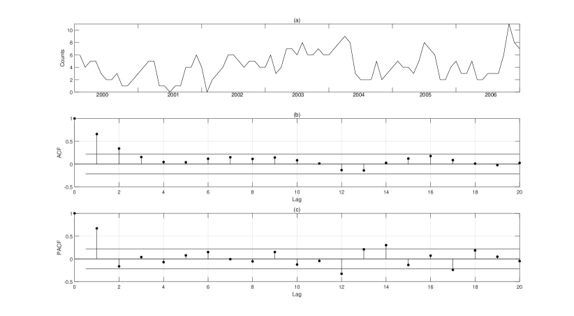
Figure 1: The sample path, ACF and PACF of the download counts
(from January 2000 to December 2006, sample size $n=84$).

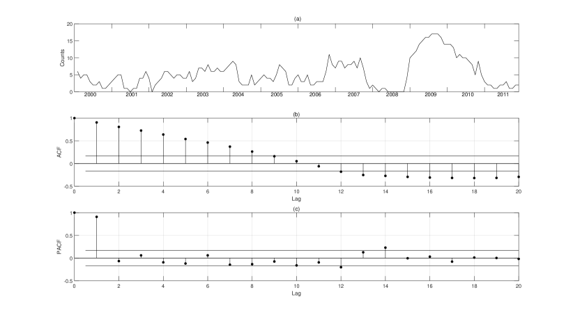
Figure 2: The sample path, ACF and PACF of the download counts
(from January 2000 to December 2011, sample size $n=143$).

Table 13: Estimators and statistics for price stability counts.

Model	Segment	$\hat{\rho}$	$\hat{p}$	$\hat{\phi}$	$\hat{\tau}$	AIC	BIC	RMS
BAR	-	0.7470	0.3079	-	-	625.5306	631.4563	1.8814
Beta-BAR(1)	-	0.3241	0.7354	0.1369	-	569.5953	578.4838	1.9018
NBAR(1)	I	0.6359	0.3197	-	107	581.0453	592.8967	1.6940
	II	0.8478	0.7784	-
MCP-BAR(1)	I	0.6140	0.2690	-	91	518.2197	541.9225	1.6413
	II	0.4464	0.0595	-	107
	III	0.7635	0.8072	-	126
	IV	0.5804	0.1446	-

6 Conclusion

The target of this article is to introduce a new BAR(1) model with multiple change-points, which is useful to handle the non-stationary count time series with a finite range. To detect the change-points, the CUSUM test is studied based on the CLS and MQL estimators. The simulation studies show that the test statistics are effective to detect change-points. Estimation for the number and locations of change-points is another important issue. For this, the MDL principle and a new algorithm named S-GA are applied. The simulation studies reveal that the adopted methods have the ability to give accurate estimators and save plenty of computing costs. Finally, an application to the price stability counts is conducted to show the superiority of the multiple change-points BAR(1) model.

Appendix

$\mathbf{Proof~{}of~{}Theorem~{}\ref{clsnormal}.}$ Note that the fact that the BAR(1) model is a strictly stationary and ergodic Markov chain and is bounded with all moments finite. Thus, it is enough to check the assumption (B2) in Theorem 3.2.24 in Taniguchi and Kakizawa (2000). Let $m(\rho,p)={\rm E}(X_{t}|\mathcal{F}_{t-1})=\rho X_{t-1}+Np(1-\rho)$. It follows that

$$\frac{\partial m(\rho,p)}{\partial\rho}=X_{t-1}-Np,~{}~{}~{}\frac{\partial m(\rho,p)}{\partial\rho}=N(1-\rho),$$

which shows that the partial derivatives of the mean function form a linearly independent system. After replacing $R$ by $\bm{W}_{CLS}$, $U$ by $\bm{V}_{CLS}$ in Theorem 3.2.24 in Taniguchi and Kakizawa (2000), Theorem 1 is easily to be proved.  
 
$\mathbf{Proof~{}of~{}Theorem~{}\ref{test1}.}$ Since $\hat{\bm{\theta}}_{n,CLS}$ satisfies the least-squares equation, by Taylor’s theorem, we obtain

$$\bm{0}=\frac{1}{\sqrt{n}}\frac{\partial S_{n}(\hat{\bm{\theta}}_{n,CLS})}{\partial\bm{\theta}}=\frac{1}{\sqrt{n}}\frac{\partial S_{n}(\bm{\theta}_{0})}{\partial\bm{\theta}}+\frac{1}{n}\frac{\partial^{2}S_{n}(\bm{\theta}_{n,CLS}^{*})}{\partial\bm{\theta}\partial\bm{\theta}^{\top}}\sqrt{n}(\hat{\bm{\theta}}_{n,CLS}-\bm{\theta}_{0}),$$ (6.1)

where $\bm{\theta}_{n,CLS}^{*}$ is an intermediate point between $\bm{\theta}_{0}$ and $\hat{\bm{\theta}}_{n,CLS}$. Denote

$$\bm{V}_{n,CLS}:=\frac{1}{2n}\frac{\partial^{2}S_{n}(\bm{\theta}_{n,CLS}^{*})}{\partial\bm{\theta}\partial\bm{\theta}^{\top}}.$$

By the ergodicity of $\{X_{t}\}$, it can be obtained that $\bm{V}_{n,CLS}\overset{\mathrm{a.s.}}{\longrightarrow}\bm{V}_{CLS}$ by using the ergodic theorem. From Equation (6.1), we have

$$\bm{V}_{CLS}\cdot\sqrt{n}(\hat{\bm{\theta}}_{n,CLS}-\bm{\theta}_{0})=-\frac{1}{2\sqrt{n}}\frac{\partial S_{n}(\bm{\theta}_{0})}{\partial\bm{\theta}}+\left\{\bm{V}_{CLS}-\bm{V}_{n,CLS}\right\}\cdot\sqrt{n}(\hat{\bm{\theta}}_{n,CLS}-\bm{\theta}_{0}).$$ (6.2)

Furthermore, if the inverse matrix of $\bm{V}_{n,CLS}$ exists, we have

$$\sqrt{n}(\hat{\bm{\theta}}_{n,CLS}-\bm{\theta}_{0})=-\left(\bm{V}_{n,CLS}\right)^{-1}\cdot\frac{1}{2\sqrt{n}}\frac{\partial S_{n}(\bm{\theta}_{0})}{\partial\bm{\theta}},$$

then

$$\bm{V}_{CLS}\cdot\sqrt{n}(\hat{\bm{\theta}}_{n,CLS}-\bm{\theta}_{0})= -\frac{1}{2\sqrt{n}}\frac{\partial S_{n}(\bm{\theta}_{0})}{\partial\bm{\theta}}$$

$$-\left(\bm{V}_{CLS}-\bm{V}_{n,CLS}\right)\cdot\left(\bm{V}_{n,CLS}\right)^{-1}\cdot\frac{1}{2\sqrt{n}}\frac{\partial S_{n}(\bm{\theta}_{0})}{\partial\bm{\theta}}.$$ (6.3)

According to Equations (6.2) and (Appendix), we can rewrite that for $0\leqslant\lambda\leqslant 1$,

$$\bm{V}_{CLS}\cdot\frac{[n\lambda]}{\sqrt{n}}(\hat{\bm{\theta}}_{[n\lambda],CLS}-\hat{\bm{\theta}}_{n,CLS})= -\frac{1}{2\sqrt{n}}\frac{\partial S_{[n\lambda]}(\bm{\theta}_{0})}{\partial\bm{\theta}}-\frac{[n\lambda]}{n}\left(-\frac{1}{2\sqrt{n}}\frac{\partial S_{n}(\bm{\theta}_{0})}{\partial\bm{\theta}}\right)$$

$$+\sqrt{\frac{[n\lambda]}{n}}\Delta_{[n\lambda]}-\frac{[n\lambda]}{n}\Delta_{n},$$ (6.4)

where

$$\Delta_{k}=\begin{cases}-\left(\bm{V}_{CLS}-\bm{V}_{k,CLS}\right)\cdot\left(\bm{V}_{k,CLS}\right)^{-1}\cdot\frac{1}{2\sqrt{k}}\frac{\partial S_{k}(\bm{\theta}_{0})}{\partial\bm{\theta}},~{}\text{if}~{}\bm{V}_{k,CLS}^{-1}~{}\text{exists},\\ \left(\bm{V}_{CLS}-\bm{V}_{k,CLS}\right)\cdot\sqrt{k}(\hat{\bm{\theta}}_{k,CLS}-\bm{\theta}_{0}),~{}\text{otherwise.}\end{cases}$$

It is easy to check that $\mathrm{E}[\partial S_{k}(\bm{\theta}_{0})/\partial\bm{\theta}|\mathcal{F}_{k-1}]={\bm{0}}$. As seen in Lee et al. (2003), the functional limit theorem for martingales is a key tool to verify the asymptotic results for the CUSUM test, coupled with the fact that $\bm{W}_{CLS}$ is a positive definite matrix under $\mathcal{H}_{0}$, there is

$$-\bm{W}_{CLS}^{-1/2}\frac{1}{2\sqrt{n}}\frac{\partial S_{[n\lambda]}(\bm{\theta}_{0})}{\partial\bm{\theta}}\mathop{\longrightarrow}\limits^{\mathrm{d}}\mathbf{B}_{2}^{\circ}(\lambda),$$ (6.5)

where $\mathbf{B}_{2}^{\circ}(\lambda)=(B_{1}^{\circ}(\lambda),B_{2}^{\circ}(\lambda))^{\top}$ is a two-dimensional standard Brownian motion. Building upon Lemma 1, which asserts that

$$\max_{1\leqslant k\leqslant n}\sqrt{\frac{k}{n}}||\Delta_{k}||=o_{p}(1),$$

and integrating the results from (Appendix) and (6.5), we have

$$\bm{W}_{CLS}^{-1/2}\bm{V}_{CLS}\frac{[n\lambda]}{\sqrt{n}}(\hat{\bm{\theta}}_{[n\lambda],CLS}-\hat{\bm{\theta}}_{n,CLS})\mathop{\longrightarrow}\limits^{\mathrm{d}}\bm{B}_{2}(\lambda).$$

The proof of Theorem 2 has been completed.  
 
$\mathbf{Proof~{}of~{}Theorem~{}\ref{the_cls_c}.}$ Following Theorem 2, the result in Theorem 3 under $\mathcal{H}_{0}$ is obviously true. Inspired by the proof of Theorem 2 in Pešta and Wendler (2020), we next prove the result in Theorem 3 under $\mathcal{H}_{1}$, i.e,

$$C_{n}^{CLS}\mathop{\longrightarrow}\limits^{\mathrm{p}}+\infty,~{}~{}n\rightarrow\infty.$$

Without loss of generality, we assume that the sequence $\{X_{t}\}_{t=1}^{n}$ has only one change point at $t=\tau$, and denote $\lambda=\tau/n$ with $0<\lambda<1$. It follows that we can divide the sequence $\{X_{t}\}_{t=1}^{n}$ into two stationary sequences, $\{X_{t}\}_{t=1}^{\tau}$ and $\{X_{t}\}_{t=\tau+1}^{n}$, which are generated from the BAR(1) model (1.1) depending on $\bm{\theta}_{1}$ and $\bm{\theta}_{2}$ with $\bm{\theta}_{1}\neq\bm{\theta}_{2}$, respectively. According to the definition of $C_{n}^{CLS}$, we have

$$C_{n}^{CLS}\geqslant C_{n,\tau}^{CLS}=\frac{\tau^{2}}{n}(\hat{\bm{\theta}}_{\tau,CLS}-\hat{\bm{\theta}}_{n,CLS})^{\top}\hat{\bm{V}}_{n,CLS}\hat{\bm{W}}_{n,CLS}^{-1}\hat{\bm{V}}_{n,CLS}(\hat{\bm{\theta}}_{\tau,CLS}-\hat{\bm{\theta}}_{n,CLS}).$$

Following the asymptotic proprieties of the CLS estimator, we have $\hat{\bm{\theta}}_{\tau,CLS}\mathop{\longrightarrow}\limits^{\mathrm{a.s.}}\bm{\theta}_{1}$, as $n\rightarrow\infty$. Also, since $\bm{\theta}_{1}\neq\bm{\theta}_{2}$, the asymptotic proprieties imply that

$$||\hat{\bm{\theta}}_{\tau,CLS}-\hat{\bm{\theta}}_{n,CLS}||\neq 0,~{}~{}n\rightarrow\infty.$$

Notably, the determinant of $\hat{\bm{V}}_{n,CLS}$ is given by

$$|\hat{\bm{V}}_{n,CLS}| =N^{2}(1-\hat{\rho}_{n,CLS})^{2}\frac{1}{n}\sum_{t=1}^{n}(X_{t-1}-N\hat{p}_{n,CLS})^{2}-\left[\frac{1}{n}\sum_{t=1}^{n}(X_{t-1}-N\hat{p}_{n,CLS})N(1-\hat{\rho}_{n,CLS})\right]^{2}$$

$$=N^{2}(1-\hat{\rho}_{n,CLS})^{2}\left\{\frac{1}{n}\sum_{t=1}^{n}(X_{t-1}-N\hat{p}_{n,CLS})^{2}-\left[\frac{1}{n}\sum_{t=1}^{n}(X_{t-1}-N\hat{p}_{n,CLS})\right]^{2}\right\}.$$

Clearly, $|\hat{\bm{V}}_{n,CLS}|\neq 0$. Similarly, we can verify $|\hat{\bm{W}}_{n,CLS}|\neq 0$. Thus, there exist a constant $c\neq 0$ such that

$$C_{n}^{CLS} \geqslant C_{n,\tau}^{CLS}=\lambda([n\lambda])(\hat{\bm{\theta}}_{\tau,CLS}-\hat{\bm{\theta}}_{n,CLS})^{\top}\hat{\bm{V}}_{n,CLS}\hat{\bm{W}}_{n,CLS}^{-1}\hat{\bm{V}}_{n,CLS}(\hat{\bm{\theta}}_{\tau,CLS}-\hat{\bm{\theta}}_{n,CLS})$$

$$\geqslant c\lambda[n\lambda]\mathop{\longrightarrow}\limits^{\mathrm{p}}+\infty,~{}~{}n\rightarrow\infty.$$

That is, $C_{n}^{CLS}\mathop{\longrightarrow}\limits^{\mathrm{p}}+\infty,$ as $n\rightarrow\infty$. The proof of Theorem 3 has been completed.
 
$\mathbf{Proof~{}of~{}Theorem~{}\ref{the_qml_c}.}$ The proof is similar to the proof of Theorem 3, and we omit it.
 
$\mathbf{Expression~{}in~{}Theorem~{}\ref{the_qml_c}.}$ Let $k_{0}$ be a positive integer, and define

$$C_{n}^{MQL}=\max_{k_{0}\leqslant k\leqslant n}\frac{k^{2}}{n}(\hat{\bm{\theta}}_{k,MQL}-\hat{\bm{\theta}}_{n,MQL})^{\top}\hat{\bm{V}}_{n,MQL}\hat{\bm{W}}_{n,MQL}^{-1}\hat{\bm{V}}_{n,MQL}(\hat{\bm{\theta}}_{k,MQL}-\hat{\bm{\theta}}_{n,MQL}).$$

where

$$\small\hat{\bm{V}}_{n,MQL}=\left({\begin{array}[]{lc}\hat{{V}}_{n,MQL}^{(1,1)}&\hat{{V}}_{n,MQL}^{(1,2)}\\ \hat{{V}}_{n,MQL}^{(2,1)}&\hat{{V}}_{n,MQL}^{(2,2)}\end{array}}\right),~{}~{}~{}\hat{\bm{W}}_{n,MQL}=\left({\begin{array}[]{*{2}{c}}\hat{{W}}_{n,MQL}^{(1,1)}&\hat{{W}}_{n,MQL}^{(1,2)}\\ \hat{{W}}_{n,MQL}^{(2,1)}&\hat{{W}}_{n,MQL}^{(2,2)}\end{array}}\right)$$

with

$$\hat{{V}}_{n,MQL}^{(1,1)}={\frac{1}{n}\sum\limits_{t=1}^{n}D_{t}(\hat{\bm{\theta}}_{n,CLS})(X_{t-1}-N\hat{p}_{n,MQL})^{2}},$$

$$\hat{{V}}_{n,MQL}^{(1,2)}=\hat{{V}}_{n,MQL}^{(2,1)}={\frac{1}{n}\sum\limits_{t=1}^{n}D_{t}(\hat{\bm{\theta}}_{n,CLS})\big{\{}(X_{t-1}-N\hat{p}_{n,MQL})(N(1-\hat{\rho}_{n,MQL})+s_{t}(\bm{\theta}_{n,MQL})]\big{\}}},$$

$$\hat{{V}}_{n,MQL}^{(2,2)}={N^{2}(1-\hat{\rho}_{n,MQL})^{2}\frac{1}{n}\sum\limits_{t=1}^{n}D_{t}(\hat{\bm{\theta}}_{n,CLS})},$$

$$\hat{{W}}_{n,MQL}^{(1,1)}={\frac{1}{n}\sum_{t=1}^{n}[D_{t}(\hat{\bm{\theta}}_{n,CLS})s_{t}(\hat{\bm{\theta}}_{n,MQL})(X_{t-1}-N\hat{p}_{n,MQL})]^{2}},$$

$$\hat{{W}}_{n,MQL}^{(1,2)}=\hat{{W}}_{n,MQL}^{(2,1)}={\frac{1}{n}\sum_{t=1}^{n}[D_{t}(\hat{\bm{\theta}}_{n,CLS})s_{t}(\hat{\bm{\theta}}_{n,MQL})]^{2}(X_{t-1}-N\hat{p}_{n,MQL})N(1-\hat{\rho}_{n,MQL})},$$

$$\hat{{W}}_{n,MQL}^{(2,2)}={\frac{1}{n}\sum_{t=1}^{n}[D_{t}(\hat{\bm{\theta}}_{n,CLS})s_{t}(\hat{\bm{\theta}}_{n,MQL})N(1-\hat{\rho}_{n,MQL})]^{2}}.$$

$\mathbf{Proof~{}of~{}Theorem~{}\ref{the_cml_c}.}$ The proof is similar to the proof of Theorem 3, and we omit it.
 
$\mathbf{Fisher~{}information~{}matrix~{}Expression~{}in~{}Theorem~{}\ref{the_cml_c}.}$ Recall that the transition probabilities of the BAR(1) model is given by

$$\mathrm{P}(X_{t}|X_{t-1}) =\sum_{k=\max\{0,X_{t-1}+X_{t}-N\}}^{\min\{X_{t-1},X_{t}\}}\binom{X_{t-1}}{k}\binom{N-X_{t-1}}{X_{t}-k}\alpha^{k}(1-\alpha)^{X_{t-1}-k}\beta^{X_{t}-k}(1-\beta)^{N-X_{t-1}-X_{t}+k},$$

$$=:\sum_{k=\Delta_{1}}^{\Delta_{2}}J_{0}(k)J_{1}(k,\bm{\theta})J_{2}(k,\bm{\theta})J_{3}(k,\bm{\theta})J_{4}(k,\bm{\theta}),$$

where

$$J_{0}(k)=\binom{X_{t-1}}{k}\binom{N-X_{t-1}}{X_{t}-k},\Delta_{1}=\max\{0,X_{t-1}+X_{t}-N\},\Delta_{2}=\min\{X_{t-1},X_{t}\},$$

$$J_{1}(k,\bm{\theta})=\alpha^{k},J_{2}(k,\bm{\theta})=(1-\alpha)^{X_{t-1}-k},J_{3}(k,\bm{\theta})=\beta^{X_{t}-k},J_{4}(k,\bm{\theta})=(1-\beta)^{N-X_{t-1}-X_{t}+k}.$$

It follows that

$$\frac{\partial J_{1}(k,\bm{\theta})}{\partial\rho}=k\alpha^{k-1}(1-p),~{}~{}~{}\frac{\partial J_{1}(k,\bm{\theta})}{\partial p}=k\alpha^{k-1}(1-\rho),$$

$$\frac{\partial J_{2}(k,\bm{\theta})}{\partial\rho}=-(X_{t-1}-k)(1-\alpha)^{X_{t-1}-k-1}(1-p),$$

$$\frac{\partial J_{2}(k,\bm{\theta})}{\partial p}=-(X_{t-1}-k)(1-\alpha)^{X_{t-1}-k-1}(1-\rho),$$

$$\frac{\partial J_{3}(k,\bm{\theta})}{\partial\rho}=({X_{t}-k})\beta^{X_{t}-k-1}(-p),~{}~{}~{}\frac{\partial J_{3}(k,\bm{\theta})}{\partial p}=({X_{t}-k})\beta^{X_{t}-k-1}(1-\rho),$$

$$\frac{\partial J_{4}(k,\bm{\theta})}{\partial\rho}=-({N-X_{t-1}-X_{t}+k})(1-\beta)^{N-X_{t-1}-X_{t}+k-1}(-p),$$

$$\frac{\partial J_{4}(k,\bm{\theta})}{\partial p}=-({N-X_{t-1}-X_{t}+k})(1-\beta)^{N-X_{t-1}-X_{t}+k-1}(1-\rho).$$

After a simple calculation, there is

$${\rm P}_{\rho}^{{}^{\prime}}(k,\bm{\theta})= \frac{\partial\mathrm{P}(X_{t}|X_{t-1})}{\partial\rho}=\sum_{k=\Delta_{1}}^{\Delta_{2}}J_{0}(k)\Big{[}\frac{\partial J_{1}(k,\bm{\theta})}{\partial\rho}J_{2}(k,\bm{\theta})J_{3}(k,\bm{\theta})J_{4}(k,\bm{\theta})$$

$$+\frac{\partial J_{2}(k,\bm{\theta})}{\partial\rho}J_{1}(k,\bm{\theta})J_{3}(k,\bm{\theta})J_{4}(k,\bm{\theta})+\frac{\partial J_{3}(k,\bm{\theta})}{\partial\rho}J_{1}(k,\bm{\theta})J_{2}(k,\bm{\theta})J_{4}(k,\bm{\theta})$$

$$+\frac{\partial J_{4}(k,\bm{\theta})}{\partial\rho}J_{1}(k,\bm{\theta})J_{2}(k,\bm{\theta})J_{3}(k,\bm{\theta})\Big{]},$$

$${\rm P}_{p}^{{}^{\prime}}(k,\bm{\theta})= \frac{\partial\mathrm{P}(X_{t}|X_{t-1})}{\partial p}=\sum_{k=\Delta_{1}}^{\Delta_{2}}J_{0}(k)\Big{[}\frac{\partial J_{1}(k,\bm{\theta})}{\partial p}J_{2}(k,\bm{\theta})J_{3}(k,\bm{\theta})J_{4}(k,\bm{\theta})$$

$$+\frac{\partial J_{2}(k,\bm{\theta})}{\partial p}J_{1}(k,\bm{\theta})J_{3}(k,\bm{\theta})J_{4}(k,\bm{\theta})+\frac{\partial J_{3}(k,\bm{\theta})}{\partial p}J_{1}(k,\bm{\theta})J_{2}(k,\bm{\theta})J_{4}(k,\bm{\theta})$$

$$+\frac{\partial J_{4}(k,\bm{\theta})}{\partial p}J_{1}(k,\bm{\theta})J_{2}(k,\bm{\theta})J_{3}(k,\bm{\theta})\Big{]}.$$

Furthermore, there is

$$\frac{\partial^{2}J_{1}(k,\bm{\theta})}{\partial\rho^{2}}=k({k-1})\alpha^{k-2}(1-p)^{2},~{}~{}\frac{\partial^{2}J_{1}(k,\bm{\theta})}{\partial p^{2}}=k({k-1})\alpha^{k-2}(1-\rho)^{2},$$

$$\frac{\partial^{2}J_{1}(k,\bm{\theta})}{\partial\rho\partial p}=\frac{\partial^{2}J_{1}(k,\bm{\theta})}{\partial p\partial\rho}=k({k-1})(\alpha)^{k-2}(1-p)(1-\rho)-k\alpha^{k-1},$$

$$\frac{\partial^{2}J_{2}(k,\bm{\theta})}{\partial\rho^{2}}=({X_{t-1}-k-1})(X_{t-1}-k)(1-\alpha)^{X_{t-1}-k-2}(1-p)^{2},$$

$$\frac{\partial^{2}J_{2}(k,\bm{\theta})}{\partial p^{2}}=({X_{t-1}-k-1})(X_{t-1}-k)(1-\alpha)^{X_{t-1}-k-2}(1-\rho)^{2},$$

$$\frac{\partial^{2}J_{2}(k,\bm{\theta})}{\partial\rho\partial p}=\frac{\partial^{2}J_{2}(k,\bm{\theta})}{\partial p\partial\rho}=({X_{t-1}-k-1})(X_{t-1}-k)(1-\alpha)^{X_{t-1}-k-2}(1-p)(1-\rho)$$

$$~{}~{}~{}~{}~{}~{}~{}~{}~{}~{}~{}~{}~{}~{}~{}~{}~{}~{}~{}~{}~{}~{}~{}~{}~{}~{}~{}~{}~{}~{}~{}~{}~{}~{}~{}+(X_{t-1}-k)(1-\alpha)^{X_{t-1}-k-1},$$

$$\frac{\partial^{2}J_{3}(k,\bm{\theta})}{\partial\rho^{2}}=({X_{t}-k-1})({X_{t}-k})\beta^{X_{t}-k-2}p^{2},$$

$$\frac{\partial^{2}J_{3}(k,\bm{\theta})}{\partial p^{2}}=({X_{t}-k-1})({X_{t}-k})\beta^{X_{t}-k-2}(1-\rho)^{2},$$

$$\frac{\partial^{2}J_{3}(k,\bm{\theta})}{\partial\rho\partial p}=\frac{\partial^{2}J_{3}(k,\bm{\theta})}{\partial p\partial\rho}=({X_{t}-k-1})({X_{t}-k})\beta^{X_{t}-k-2}p(\rho-1)-({X_{t}-k})\beta^{X_{t}-k-1},$$

$$\frac{\partial^{2}J_{4}(k,\bm{\theta})}{\partial\rho^{2}}=({N-X_{t-1}-X_{t}+k-1})({N-X_{t-1}-X_{t}+k})(1-\beta)^{N-X_{t-1}-X_{t}+k-2}p^{2},$$

$$\frac{\partial^{2}J_{4}(k,\bm{\theta})}{\partial p^{2}}=({N-X_{t-1}-X_{t}+k-1})({N-X_{t-1}-X_{t}+k})(1-\beta)^{N-X_{t-1}-X_{t}+k-2}(1-\rho)^{2},$$

$$\frac{\partial^{2}J_{4}(k,\bm{\theta})}{\partial\rho\partial p}=\frac{\partial^{2}J_{4}(k,\bm{\theta})}{\partial p\partial\rho}=({N-X_{t-1}-X_{t}+k-1})({N-X_{t-1}-X_{t}+k})(1-\beta)^{N-X_{t-1}-X_{t}+k-2}$$

$$~{}~{}~{}~{}~{}~{}~{}~{}~{}~{}~{}~{}~{}~{}~{}~{}~{}~{}~{}~{}~{}~{}~{}~{}~{}~{}~{}~{}~{}~{}~{}~{}~{}~{}~{}\times p(\rho-1)+({N-X_{t-1}-X_{t}+k})(1-\beta)^{N-X_{t-1}-X_{t}+k-1}.$$

Denote

$$A_{1j}(k,\bm{\theta})= \frac{\partial^{2}J_{j}(k,\bm{\theta})}{\partial\rho^{2}}\prod_{s_{1}=1,\hfill\atop s_{1}\neq j}^{4}J_{s_{1}}(k,\bm{\theta})+\frac{\partial J_{j}(k,\bm{\theta})}{\partial\rho}\left[\sum_{s_{2}=1,\hfill\atop s_{2}\neq j}^{4}\left(\frac{\partial J_{s_{2}}(k,\bm{\theta})}{\partial\rho}\prod_{s_{3}=1,\hfill s_{3}\neq s_{2},\atop s_{3}\neq j}^{4}J_{s_{3}}(k,\bm{\theta})\right)\right],$$

$$A_{2j}(k,\bm{\theta})= \frac{\partial^{2}J_{j}(k,\bm{\theta})}{\partial\rho\partial p}\prod_{s_{1}=1,\hfill\atop s_{1}\neq j}^{4}J_{s_{1}}(k,\bm{\theta})+\frac{\partial J_{j}(k,\bm{\theta})}{\partial\rho}\left[\sum_{s_{2}=1,\hfill\atop s_{2}\neq j}^{4}\left(\frac{\partial J_{s_{2}}(k,\bm{\theta})}{\partial p}\prod_{s_{3}=1,\hfill s_{3}\neq s_{2},\atop s_{3}\neq j}^{4}J_{s_{3}}(k,\bm{\theta})\right)\right],$$

$$A_{3j}(k,\bm{\theta})= \frac{\partial^{2}J_{j}(k,\bm{\theta})}{\partial p^{2}}\prod_{s_{1}=1,\hfill\atop s_{1}\neq j}^{4}J_{s_{1}}(k,\bm{\theta})+\frac{\partial J_{j}(k,\bm{\theta})}{\partial p}\left[\sum_{s_{2}=1,\hfill\atop s_{2}\neq j}^{4}\left(\frac{\partial J_{s_{2}}(k,\bm{\theta})}{\partial p}\prod_{s_{3}=1,\hfill s_{3}\neq s_{2},\atop s_{3}\neq j}^{4}J_{s_{3}}(k,\bm{\theta})\right)\right],$$

where $j=1,2,3,4$. Then, after some simple calculations, there is

$${\rm P}_{\rho}^{{}^{\prime\prime}}(k,\bm{\theta})=\frac{\partial^{2}\mathrm{P}(X_{t}|X_{t-1})}{\partial\rho^{2}}=\sum_{k=\Delta_{1}}^{\Delta_{2}}J_{0}(k)\left[A_{11}(k,\bm{\theta})+A_{12}(k,\bm{\theta})+A_{13}(k,\bm{\theta})+A_{14}(k,\bm{\theta})\right],$$

$${\rm P}_{\rho,p}^{{}^{\prime\prime}}(k,\bm{\theta})=\frac{\partial^{2}\mathrm{P}(X_{t}|X_{t-1})}{\partial\rho\partial p}=\frac{\partial^{2}\mathrm{P}(X_{t}|X_{t-1})}{\partial p\partial\rho}$$

$$~{}~{}~{}~{}~{}~{}~{}~{}~{}~{}~{}~{}=\sum_{k=\Delta_{1}}^{\Delta_{2}}J_{0}(k)\left[A_{21}(k,\bm{\theta})+A_{22}(k,\bm{\theta})+A_{23}(k,\bm{\theta})+A_{24}(k,\bm{\theta})\right],$$

$${\rm P}_{p}^{{}^{\prime\prime}}(k,\bm{\theta})=\frac{\partial^{2}\mathrm{P}(X_{t}|X_{t-1})}{\partial p^{2}}=\sum_{k=\Delta_{1}}^{\Delta_{2}}J_{0}(k)\left[A_{31}(k,\bm{\theta})+A_{32}(k,\bm{\theta})+A_{33}(k,\bm{\theta})+A_{34}(k,\bm{\theta})\right].$$

Recall that the Fisher information matrix is

$$\bm{I}^{-1}(\bm{\theta}_{0})=\mathrm{E}\left[-\frac{\partial^{2}\ell_{t}(\bm{\theta}_{0}|X_{t-1})}{\partial\bm{\theta}\partial\bm{\theta}^{\mathrm{T}}}\right].$$

Clearly, according to the ergodicity of the BAR(1) model, the consistent estimator of $\bm{I}^{-1}(\bm{\theta}_{0})$ is given by

$$\hat{\bm{I}}_{n,CML}^{-1}=\left({\begin{array}[]{*{2}{c}}\hat{I}_{n,CML}^{(1,1)}&\hat{I}_{n,CML}^{(1,2)}\\ \hat{I}_{n,CML}^{(1,2)}&\hat{I}_{n,CML}^{(2,2)}\end{array}}\right),$$

where

$$\hat{I}_{n,CML}^{(1,1)} =\frac{1}{n}\sum_{t=1}^{n}\left\{-\frac{1}{\left(\mathrm{P}(X_{t}|X_{t-1})\right)^{2}}\left[{\rm P}_{\rho}^{{}^{\prime}}(k,\bm{\theta})\right]^{2}+\frac{1}{\mathrm{P}(X_{t}|X_{t-1})}{\rm P}_{\rho}^{{}^{\prime\prime}}(k,\bm{\theta})\right\}_{\bm{\theta}=\hat{\bm{\theta}}_{n,CML}},$$

$$\hat{I}_{n,CML}^{(1,2)} =\frac{1}{n}\sum_{t=1}^{n}\left\{-\frac{1}{\left(\mathrm{P}(X_{t}|X_{t-1})\right)^{2}}\left[{\rm P}_{\rho}^{{}^{\prime}}(k,\bm{\theta}){\rm P}_{p}^{{}^{\prime}}(k,\bm{\theta})\right]+\frac{1}{\mathrm{P}(X_{t}|X_{t-1})}{\rm P}_{\rho,p}^{{}^{\prime\prime}}(k,\bm{\theta})\right\}_{\bm{\theta}=\hat{\bm{\theta}}_{n,CML}},$$

$$\hat{I}_{n,CML}^{(2,2)} =\frac{1}{n}\sum_{t=1}^{n}\left\{-\frac{1}{\left(\mathrm{P}(X_{t}|X_{t-1})\right)^{2}}\left[{\rm P}_{p}^{{}^{\prime}}(k,\bm{\theta})\right]^{2}+\frac{1}{\mathrm{P}(X_{t}|X_{t-1})}{\rm P}_{p}^{{}^{\prime\prime}}(k,\bm{\theta})\right\}_{\bm{\theta}=\hat{\bm{\theta}}_{n,CML}}.$$

$\mathbf{Proof~{}of~{}Theorem~{}\ref{strong}.}$ Let the time series $\{X_{t,j}\}_{t=1}^{n_{j}}$ generate from the $j$th segment BAR model. Denote the true likelihood based on the time series $\{X_{t,j}\}_{t=1}^{n_{j}}$ by

$$\widetilde{L}_{n_{j}}(0,\bm{\theta}_{j}) =\sum\limits_{t=1}^{n_{j}}\ell_{t}(\bm{\theta}_{j}|X_{s,j},s<t)=\sum\limits_{t=1}^{n_{j}}\log\mathrm{P}(X_{t,j}|X_{t-1,j}).$$ (6.6)

Denote $\sup_{\lambda_{d},\lambda_{u}}:=\sup_{\lambda_{d}\in[0,1],\lambda_{u}\in[0,1],\lambda_{u}-\lambda_{d}>\epsilon_{\lambda}}.$ Define, for $j=1,...,m+1$, the true and the observed likelihood formed by a portion of the $j$th segment respectively by

$$\widetilde{L}_{n_{j}}(\bm{\theta}_{j},\lambda_{d},\lambda_{u}) =\sum\limits_{t=[n_{j}\lambda_{d}]}^{[n_{j}\lambda_{u}]}\ell_{t}(\bm{\theta}_{j}|X_{s,j},s<t)=\sum\limits_{t=[n_{j}\lambda_{d}]}^{[n_{j}\lambda_{u}]}\log\mathrm{P}(X_{t,j}|X_{t-1,j}),$$

$$L_{n_{j}}(\bm{\theta}_{j},\lambda_{d},\lambda_{u}) =\sum\limits_{t=[n_{j}\lambda_{d}]}^{[n_{j}\lambda_{u}]}\ell_{t}(\bm{\theta}_{j}|X_{s},s<t)=\sum\limits_{t=[n_{j}\lambda_{d}]}^{[n_{j}\lambda_{u}]}\log\mathrm{P}(X_{t}|X_{t-1}).$$

To ensure the validity of Theorem 7, we confirm adherence to Assumptions 1 (2), 2 (4), 3 , 5, and either 4 (0.5) or 4* in Davis and Yau (2013). Given our focus on the first-order BAR model, Assumption 5 in Davis and Yau (2013), which is designed to ensure model selection consistency and identifiability of models, is obviously true. For easy reading, we summarize Assumptions 1($\kappa$), 2($\kappa$), 3, 4* in Davis and Yau (2013) as follows:

$\bullet$ Assumption 1($\kappa$): For any $j=1,2,...,m+1$, the function $\ell_{t}(\bm{\theta}_{j}|X_{s,j},s<t)$ is two-time continuously differentiable with respective to $\bm{\theta}_{j}$, and the first and second derivatives $\widetilde{L}_{n_{j}}^{{}^{\prime}}(\bm{\theta}_{j},\lambda_{d},\lambda_{u})$, $L_{n_{j}}^{{}^{\prime}}(\bm{\theta}_{j},\lambda_{d},\lambda_{u})$ and $\widetilde{L}_{n_{j}}^{{}^{\prime\prime}}(\bm{\theta}_{j},\lambda_{d},\lambda_{u})$, $L_{n_{j}}^{{}^{\prime\prime}}(\bm{\theta}_{j},\lambda_{d},\lambda_{u})$, respectively, of the function $\widetilde{L}_{n_{j}}(\bm{\theta}_{j},\lambda_{d},\lambda_{u})$ and $L_{n_{j}}(\bm{\theta}_{j},\lambda_{d},\lambda_{u})$, satisfy

$$\sup_{\lambda_{d},\lambda_{u}}\sup\limits_{\bm{\theta}_{j}\in\Theta_{j}}|\frac{1}{n}\widetilde{L}_{n_{j}}(\bm{\theta}_{j},\lambda_{d},\lambda_{u})-\frac{1}{n}L_{n_{j}}(\bm{\theta}_{j},\lambda_{d},\lambda_{u})| =o(n^{\frac{1}{\kappa}-1}),$$

$$\sup_{\lambda_{d},\lambda_{u}}\sup\limits_{\bm{\theta}_{j}\in\Theta_{j}}|\frac{1}{n}\widetilde{L}_{n_{j}}^{{}^{\prime}}(\bm{\theta}_{j},\lambda_{d},\lambda_{u})-\frac{1}{n}L_{n_{j}}^{{}^{\prime}}(\bm{\theta}_{j},\lambda_{d},\lambda_{u})| =o(n^{\frac{1}{\kappa}-1}),$$

$$\sup_{\lambda_{d},\lambda_{u}}\sup\limits_{\bm{\theta}_{j}\in\Theta_{j}}|\frac{1}{n}\widetilde{L}_{n_{j}}^{{}^{\prime\prime}}(\bm{\theta}_{j},\lambda_{d},\lambda_{u})-\frac{1}{n}L_{n_{j}}^{{}^{\prime\prime}}(\bm{\theta}_{j},\lambda_{d},\lambda_{u})| =o(1),$$

almost surely.

$\bullet$ Assumption 2($\kappa$): For $j=1,2,...,m+1$, there exists an $\epsilon>0$ such that

$$\sup\limits_{\bm{\theta}_{j}\in\Theta_{j}}{\rm E}|\ell_{t}(\bm{\theta}_{j}|X_{s,j},s<t)|^{\kappa+\epsilon}<\infty,$$

$$\sup\limits_{\bm{\theta}_{j}\in\Theta_{j}}{\rm E}|\ell_{t}^{{}^{\prime}}(\bm{\theta}_{j}|X_{s,j},s<t)|^{\kappa+\epsilon}<\infty,$$

$$\sup\limits_{\bm{\theta}_{j}\in\Theta_{j}}{\rm E}|\ell_{t}^{{}^{\prime\prime}}(\bm{\theta}_{j}|X_{s,j},s<t)|<\infty,$$

where $\ell_{t}^{{}^{\prime}}$ and $\ell_{t}^{{}^{\prime\prime}}$ are the first and second derivatives of $\ell_{t}$

$\bullet$ Assumption 3: For each $j=1,2,...,m+1$,

$$\sup\limits_{\bm{\theta}_{j}\in\Theta_{j}}\left|\frac{1}{n}\widetilde{L}_{n_{j}}(0,\bm{\theta}_{j})-{\rm E}[\ell_{t}(\bm{\theta}_{j}|X_{s,j},s<t)]\right|\overset{\mathrm{a.s.}}{\longrightarrow}0,$$

$$\sup\limits_{\bm{\theta}_{j}\in\Theta_{j}}\left|\frac{1}{n}\widetilde{L}_{n_{j}}^{{}^{\prime}}(0,\bm{\theta}_{j})-{\rm E}[\ell_{t}^{{}^{\prime}}(\bm{\theta}_{j}|X_{s,j},s<t)]\right|\overset{\mathrm{a.s.}}{\longrightarrow}0,$$

$$\sup\limits_{\bm{\theta}_{j}\in\Theta_{j}}\left|\frac{1}{n}\widetilde{L}_{n_{j}}^{{}^{\prime\prime}}(0,\bm{\theta}_{j})-{\rm E}[\ell_{t}^{{}^{\prime\prime}}(\bm{\theta}_{j}|X_{s,j},s<t)]\right|\overset{\mathrm{a.s.}}{\longrightarrow}0.$$

$\bullet$ Assumption 4*: For each $j$, $\{\ell_{t}(\bm{\theta}_{j}|X_{s,j},s<t);t\in\mathbb{Z}\}$ and $\{\ell_{t}^{{}^{\prime}}(\bm{\theta}_{j}|X_{s,j},s<t);t\in\mathbb{Z}\}$ are strongly mixing sequences of random variables with geometric rate.

To substantiate the aforementioned assumptions, we then divided the proof into the following three steps.
Step 1. We first prove the Assumption 1 (2) to be hold. In fact, since BAR(1) model is bounded, we can easily prove that Assumption 1 ($\kappa$) in Davis and Yau (2013) to be hold for any $\kappa\geqslant 1$. That is, for any $j=1,2,...,m+1$, the function $\ell_{t}$ is two-time continuously differentiable with respective to $\bm{\theta}_{j}$, and the first and second derivatives satisfy

$$\sup_{\lambda_{d},\lambda_{u}}\sup\limits_{\bm{\theta}_{j}\in\Theta_{j}}|\frac{1}{n}\widetilde{L}_{n_{j}}(\bm{\theta}_{j},\lambda_{d},\lambda_{u})-\frac{1}{n}L_{n_{j}}(\bm{\theta}_{j},\lambda_{d},\lambda_{u})| =o(n^{-1}),$$

$$\sup_{\lambda_{d},\lambda_{u}}\sup\limits_{\bm{\theta}_{j}\in\Theta_{j}}|\frac{1}{n}\widetilde{L}_{n_{j}}^{{}^{\prime}}(\bm{\theta}_{j},\lambda_{d},\lambda_{u})-\frac{1}{n}L_{n_{j}}^{{}^{\prime}}(\bm{\theta}_{j},\lambda_{d},\lambda_{u})| =o(n^{-1}),$$

$$\sup_{\lambda_{d},\lambda_{u}}\sup\limits_{\bm{\theta}_{j}\in\Theta_{j}}|\frac{1}{n}\widetilde{L}_{n_{j}}^{{}^{\prime\prime}}(\bm{\theta}_{j},\lambda_{d},\lambda_{u})-\frac{1}{n}L_{n_{j}}^{{}^{\prime\prime}}(\bm{\theta}_{j},\lambda_{d},\lambda_{u})| =o(1),$$

almost surely.
Step 2. Assumption 2 (4) and Assumption 3 are the regularity conditions for the conditional log-likelihood function to ensure the consistency of the maximum likelihood estimation. Where, similar to the argument in the Step 1, Assumption 2 (4) is obviously true because the BAR(1) model is bounded. Assumption 3 can be verified by the ergodic theorem and the compactness of the parameter space.
Step 3. We finally verify Assumption 4* to hold. It is well known that the BAR(1) process is a stationary ergodic Markov chain, according to the discussion on Page 101 in Basrak et al. (2002), the BAR(1) process is strongly mixing with geometric rate. As a result, $\ell_{t}(\bm{\theta}_{j}|X_{s,j},s<t)$ is strongly mixing with the same geometric rate as it is a function of finite number of the strongly mixing $X_{t,j}$’s (Theorem 14.1 of Davidson (1994)). Thus Assumption 4* holds. In fact, Lemma 1 in Davis and Yau (2013) already states that Assumption 4(0.5) in Davis and Yau (2013) holds under Assumption 2(2) and 4*. Clearly, Assumption 2(2) is true, so Assumption 4(0.5) in Davis and Yau (2013) is also satisfied. The proof of Theorem 7 is completed.

Lemma 1

Under $\mathcal{H}_{0}$, we have

$$\max_{1\leqslant k\leqslant n}\sqrt{\frac{k}{n}}\|\Delta_{k}\|=o_{p}(1).$$

$\mathbf{Proof~{}of~{}Lemma~{}\ref{lemma1}.}$ Recall that

$$\Delta_{k}=\begin{cases}-\left(\bm{V}_{CLS}-\bm{V}_{k,CLS}\right)\cdot\left(\bm{V}_{k,CLS}\right)^{-1}\cdot\frac{1}{2\sqrt{k}}\frac{\partial S_{k}(\bm{\theta}_{0})}{\partial\bm{\theta}},~{}\text{if}~{}\bm{V}_{k,CLS}^{-1}~{}\text{exists},\\ \left(\bm{V}_{CLS}-\bm{V}_{k,CLS}\right)\cdot\sqrt{k}(\hat{\bm{\theta}}_{k,CLS}-\bm{\theta}_{0}),~{}\text{otherwise.}\end{cases}$$

Note that the fact $\bm{V}_{n,CLS}\overset{a.s.}{\longrightarrow}\bm{V}_{CLS}$ as $n\rightarrow\infty$ and $\bm{V}_{CLS}$ is a positive definite matrix under $\mathcal{H}_{0}$. Therefore, it follows from Egorov’s theorem that given $\epsilon>0$ and $\delta>0$, there exists an event $E$ with ${\rm P}(E)>1-\epsilon/3$, a positive real number $\eta$, and a positive integer $n_{0}$, such that on $E$ and for all $n>n_{0}$,

$$v_{n}\geqslant\eta,$$ (6.7)

where $v_{n}$ denotes the minimum eigenvalue of $\bm{V}_{n,CLS}$, and for each $1\leqslant i,j\leqslant 2$

$$\left|\bm{V}_{CLS}^{(i,j)}-\bm{V}_{n,CLS}^{(i,j)}\right|\leqslant\delta\eta.$$ (6.8)

Since (6.7) implies the existence of $\bm{V}_{n,CLS}^{-1}$, we have that on $E$ and for all $n>n_{0}$,

$$\Delta_{n}=-\left(\bm{V}_{CLS}-\bm{V}_{n,CLS}\right)\cdot\left(\bm{V}_{n,CLS}\right)^{-1}\cdot\frac{1}{2\sqrt{n}}\frac{\partial S_{n}(\bm{\theta}_{0})}{\partial\bm{\theta}},$$

Thus, on $E$,

$$\max_{n_{0}<k\leqslant n}\sqrt{\frac{k}{n}}||\Delta_{k}||=\max_{n_{0}<k\leqslant n}\sqrt{\frac{k}{n}}\left\|\left(\bm{V}_{CLS}-\bm{V}_{k,CLS}\right)\cdot\left(\bm{V}_{k,CLS}\right)^{-1}\cdot\frac{1}{2\sqrt{k}}\frac{\partial S_{k}(\bm{\theta}_{0})}{\partial\bm{\theta}}\right\|$$

$$\leqslant\max_{n_{0}<k\leqslant n}\left\|\bm{V}_{CLS}-\bm{V}_{k,CLS}\right\|\cdot\max_{n_{0}<k\leqslant n}\left\|\left(\bm{V}_{k,CLS}\right)^{-1}\right\|\cdot\max_{n_{0}<k\leqslant n}\left\|\frac{1}{2\sqrt{n}}\frac{\partial S_{k}(\bm{\theta}_{0})}{\partial\bm{\theta}}\right\|$$

$$\leqslant\sum_{i=1}^{2}\max_{n_{0}<k\leqslant n}\left\|\bm{V}_{CLS}-\bm{V}_{k,CLS}\right\|\cdot\max_{n_{0}<k\leqslant n}\left\|\left(\bm{V}_{k,CLS}\right)^{-1}\right\|\cdot\max_{1\leqslant k\leqslant n}\left|\frac{1}{2\sqrt{n}}\frac{\partial S_{k}(\bm{\theta}_{0})}{\partial\bm{\theta}_{i}}\right|.$$ (6.9)

First, from (6.8) it holds that on $E$ and for $n>n_{0}$,

$$\left\|\bm{V}_{CLS}-\bm{V}_{n,CLS}\right\| :=\sup\left\{\left\|(\bm{V}_{CLS}-\bm{V}_{n,CLS})h\right\|:\|h\|\leqslant 1\right\}$$

$$=\sup\left\{\left(\sum_{i=1}^{2}\left(\sum_{j=1}^{2}(\bm{V}_{CLS}^{(i,j)}-\bm{V}_{n,CLS}^{(i,j)})h_{j}\right)^{2}\right)^{1/2}:\sum_{j=1}^{2}h_{j}^{2}\leqslant 1\right\}$$

$$\leqslant 2\delta\eta$$

and consequently, on $E$

$$\max_{n_{0}<k\leqslant n}\left\|\bm{V}_{CLS}-\bm{V}_{k,CLS}\right\|\leqslant 2\delta\eta.$$ (6.10)

Next, since $\bm{V}_{n,CLS}$ is a real symmetric matrix for all $n\geqslant 1$ and (6.7) holds on $E$ and for all $n>n_{0}$, we have

$$\max_{n_{0}<k\leqslant n}\left\|\left(\bm{V}_{k,CLS}\right)^{-1}\right\| =\max_{n_{0}<k\leqslant n}\left\{\text{the maximum absolute eigenvalue of}\left(\bm{V}_{k,CLS}\right)^{-1}\right\}$$

$$=\max_{n_{0}<k\leqslant n}\frac{1}{v_{n}}\leqslant\frac{1}{\eta}.$$ (6.11)

Therefore, combing equations (6.10) and (Appendix), it follows that the right-hand side of (Appendix) is no more than $\sum_{i=1}^{2}2\delta\max_{1\leqslant k\leqslant n}\left|(2\sqrt{n})^{-1}\partial S_{k}(\bm{\theta}_{0})/\partial\bm{\theta}_{i}\right|$ on $E$, and consequently,

$${\rm P}\left\{\left(\max_{n_{0}<k\leqslant n}\sqrt{\frac{k}{n}}\|\Delta_{k}\|>\frac{\epsilon}{2}\right)\bigcap E\right\} \leqslant{\rm P}\left\{\sum_{i=1}^{2}2\delta\max_{1\leqslant k\leqslant n}\left|\frac{1}{2\sqrt{n}}\frac{\partial S_{k}(\bm{\theta}_{0})}{\partial\bm{\theta}_{i}}\right|>\frac{\epsilon}{2}\right\}$$

$$\leqslant\sum_{i=1}^{2}{\rm P}\left\{\max_{1\leqslant k\leqslant n}\left|\frac{\partial S_{k}(\bm{\theta}_{0})}{\partial\bm{\theta}_{i}}\right|>\frac{\epsilon\sqrt{n}}{4\delta}\right\}$$

$$\leqslant\sum_{i=1}^{2}\frac{16\delta^{2}}{n\epsilon^{2}}{\rm E}\left(\frac{\partial S_{n}(\bm{\theta}_{0})}{\partial\bm{\theta}_{i}}\right)^{2}.$$

Clearly, under $\mathcal{H}_{0}$, there exist a constant $0<c<\infty$, such that

$$\sum_{i=1}^{2}\frac{1}{n}{\rm E}\left(\frac{\partial S_{n}(\bm{\theta}_{0})}{\partial\bm{\theta}_{i}}\right)^{2}\leqslant c.$$

Furthermore, we set $\delta\leqslant\sqrt{\epsilon^{3}/48c}$, and there is

$${\rm P}\left\{\left(\max_{n_{0}<k\leqslant n}\sqrt{\frac{k}{n}}\|\Delta_{k}\|>\frac{\epsilon}{2}\right)\bigcap E\right\}\leqslant\frac{\epsilon}{3}.$$

Notably, there exists a positive integer $n_{1}>n_{0}$, such that

$${\rm P}\left\{\max_{1\leqslant k\leqslant n_{0}}\sqrt{\frac{k}{n_{1}}}\|\Delta_{k}\|>\frac{\epsilon}{2}\right\}\leqslant\frac{\epsilon}{3}.$$

Following the above derivation, we have that for all $n>n_{1}$

$${\rm P}\left\{\max_{1\leqslant k\leqslant n}\sqrt{\frac{k}{n}}\|\Delta_{k}\|>\epsilon\right\}\leqslant {\rm P}\left\{\max_{1\leqslant k\leqslant n_{0}}\sqrt{\frac{k}{n}}\|\Delta_{k}\|+\max_{n_{0}<k\leqslant n}\sqrt{\frac{k}{n}}\|\Delta_{k}\|>\epsilon\right\}$$

$$\leqslant {\rm P}\left\{\max_{1\leqslant k\leqslant n_{0}}\sqrt{\frac{k}{n}}\|\Delta_{k}\|>\frac{\epsilon}{2}\right\}$$

$$+{\rm P}\left\{\left(\max_{n_{0}<k\leqslant n}\sqrt{\frac{k}{n}}\|\Delta_{k}\|>\frac{\epsilon}{2}\right)\bigcap E\right\}+{\rm P}\{E^{c}\}\leqslant\epsilon,$$

which implies

$$\max_{1\leqslant k\leqslant n}\sqrt{\frac{k}{n}}\|\Delta_{k}\|=o_{p}(1).$$

The proof of Lemma 1 is completed.  
 
Searching algorithm based on genetic algorithm

S step:
Input:	The random sample $\{x_{1},x_{2},...,x_{n}\}$ from the MCP-BAR(1) model.
	The upper bound $N$ in MCP-BAR(1) model.
	The upper bound of the number of change-points $M_{0}$.
	The sample size $n$.
Initialise:	Let ∗$\textbf{MDL-best}_{1}=\min\limits_{\bm{\tau},\bm{\theta}}\textbf{MDL}(1,\frac{\bm{\tau}}{n},\bm{\theta})$, where MDL is defined by (3.3);
	Let $\hat{m}=1$, and $(\hat{\bm{\tau}},\hat{\bm{\theta}})=\arg\min\limits_{\bm{\tau},\bm{\theta}}\textbf{MDL}(1,\frac{\bm{\tau}}{n},\bm{\theta})$.
Iterate:	for $j=2:M_{0}$
	Let ∗$\textbf{MDL-best}_{2}=\min\limits_{\bm{\tau},\bm{\theta}}\textbf{MDL}(j,\frac{\bm{\tau}}{n},\bm{\theta})$.
	Let $(\hat{\bm{\tau}}^{\star},\hat{\bm{\theta}}^{\star})=\arg\min\limits_{\bm{\tau},\bm{\theta}}\textbf{MDL}(j,\frac{\bm{\tau}}{n},\bm{\theta})$.
	if $\textbf{MDL-best}_{2}>\textbf{MDL-best}_{1}$
	break.
	else
	$\textbf{MDL-best}_{1}=\textbf{MDL-best}_{2}$.
	$\hat{m}=j$, and $(\hat{\bm{\tau}},\hat{\bm{\theta}})=(\hat{\bm{\tau}}^{\star},\hat{\bm{\theta}}^{\star})$.
	end
	end
Output:	change-points estimator $(\hat{m},\hat{\bm{\tau}},\hat{\bm{\theta}})$.

${}^{\ast}\textbf{GA step:}$
Step 1: If $\bm{\tau}$ is given, the estimator for the $j$th segment parameter $\hat{\bm{\theta}}_{j}$ can be easily obtained by the closed-form expressions or solved by MATLAB function “fmincon”.
Step 2: Use “ga” function in MATLAB to get the global optimal solution $\hat{\bm{\tau}}$.
∗When $(m,\bm{\tau})$ is fixed, parameter estimation for each segment of our model is a conventional optimization problem. We divided the estimation procedure into the above two steps.

Setting tips for Step 1 and Step 2:

1. Since the closed-form of the estimators will greatly improve the computation speed, we minimized MDL based on the CML likelihood function evaluated at CLS estimators (2.2) in Step 1.

2. The options of “ga” function is set as: “options$=$gaoptimset(‘PlotFcns’,{@gaplotbestf},‘Popula
   tionSize’,10*$s$, ‘CrossoverFraction’, 0.55, ‘Generations’, 300)”, where ‘PopulationSize’ is the size of the population, ‘CrossoverFraction’ (CF) is the fraction of the population at the next generation, not including elite children, that the crossover function creates. Later in Section 5, we will do the sensitivity analysis of the tunning parameter CF.

3. To satisfy the Assumption 1: each segment must have a sufficient number of observations, the following restriction is given when we carry out Step 2:
   if $\min(\hat{\tau}_{i+1}-\hat{\tau}_{i})<n*\epsilon_{\lambda},(i=1,...,j)$, we set MDL$(\cdot,(\hat{\tau}_{1},...,\hat{\tau}_{j}),\cdot)=\text{INF}$. In simulation, we set $\epsilon_{\lambda}=10/n.$

References

• Al-Osh and Alzaid (1987) Al-Osh, M.A., Alzaid, A.A. (1987). First-order integer-valued autoregressive (INAR(1)) process. Journal of Time Series Analysis, 8, 261-275.
• Aminikhanghahi and Cook (2017) Aminikhanghahi, S., Cook, D.J. (2017). A survey of methods for time series change point detection. Knowledge and Information Systems, 51, 339-367.
• Aue and Horváth (2013) Aue, A., Horváth, L. (2013). Structural breaks in time series. Journal of Time Series Analysis, 34, 1-16.
• Barreto-Souza (2019) Barreto-Souza, W. (2019). Mixed Poisson INAR(1) processes. Statistical Papers, 60, 2119-2139.
• Basrak et al. (2002) Basrak, B., Davis, R.A., Mikosch, T. (2002). Regular variation of GARCH processes. Stochastic Processes and their Applications, 99, 95-115.
• Boysen et al. (2009) Boysen, L., Kempe, A., Liebscher, V., Munk, A., Wittich, O. (2009). Consistencies and rates of convergence of jump-penalized least squares estimators. The Annals of Statistics, 37, 157-183.
• Chattopadhyay et al. (2021) Chattopadhyay, S., Maiti, R., Das, S., Biswas, A. (2021). Change-point analysis through integer-valued autoregressive process with application to some COVID-19 data. Statistica Neerlandica, 76, 4-34.
• Chen et al. (2023) Chen, H., Ren, H., Yao, F., Zou, C. (2023). Data-driven selection of the number of change-points via error rate control. Journal of the American Statistical Association, 118, 1415-1428.
• Darolles et al. (2019) Darolles, S., Le, Fol. G., Lu, Y., Sun, R. (2019). Bivariate integer-autoregressive process with an application to mutual fund flows. Journal of Multivariate Analysis, 173, 181-203.
• Davidson (1994) Davidson, J. (1994). Stochastic Limit Theory. Oxford: Oxford University Press.
• Davis et al. (2006) Davis, R.A., Lee, T.C.M., Rodriguez-Yam, G.A. (2006). Structural break estimation for nonstationary time series models. Journal of the American Statistical Association, 101, 223-239.
• Davis and Yau (2013) Davis, R.A., Yau, C.Y. (2013). Consistency of minimum description length model selection for piecewise stationary time series models. Electronic Journal of Statistics, 7, 381-411.
• Fernández-Fontelo et al. (2016) Fernández-Fontelo, A., Cabaña, A., Puig, P., Moriña, D. (2016). Under-reported data analysis with INAR-hidden Markov chains. Statistics in Medicine, 35, 4875-4890.
• Fernández-Fontelo et al. (2021) Fernández-Fontelo, A., Cabaña, A., Joe, H., Puig, P., Moriña, D. (2021). Untangling serially dependent underreported count data for gender-based violence. Statistics in Medicine, 38, 4404-4422.
• Freeland and McCabe (2004b) Freeland, R.K., McCabe, B.P.M. (2004b). Forecasting discrete valued low count time series. International Journal of Forecasting, 20, 427-434.
• Fryzlewicz (2014) Fryzlewicz, P. (2014). Wild binary segmentation for multiple change-point detection. The Annals of Statistics, 42, 2243-2281.
• Gourieroux and Jasiak (2004) Gourieroux, C., Jasiak, J. (2004). Heterogeneous INAR(1) model with application to car insurance. Insurance: Mathematics and Economics, 34, 177-192.
• Gouveia et al. (2018) Gouveia, S., Möller, T.A., Wei$\ss$, C.H., Scotto, M.G. (2018). A full ARMA model for counts with bounded support and its application to rainy-days time series. Stochastic Environmental Research and Risk Assessment, 32, 2495-2514.
• Guan and Hu (2022) Guan, G., Hu, X. (2022). On the analysis of a discrete-time risk model with INAR(1) processes. Scandinavian Actuarial Journal, 2022, 115-138.
• Henderson and Rathouz (2018) Henderson, N.C., Rathouz, P.J. (2018). AR(1) latent class models for longitudinal count data. Statistics in Medicine, 37, 4441-4456.
• Jackson et al. (2005) Jackson, B., Sargle, J. D., Barnes, D., Arabhi, S., Alt, A., Gioumousis, P., Gwin, E., Sangtrakulcharoen, P., Tan, L., Tsai, T.T. (2005). An algorithm for optimal partitioning of data on an interval. IEEE Signal Processing Letters, 12, 105-108.
• Jandhyala et al. (2013) Jandhyala, V., Fotopoulos, S., MacNeill, I., Liu, P. (2013). Inference for single and multiple change-points in time series. Journal of Time Series Analysis, 34, 423-446.
• Jentsch and Wei$\ss$ (2019) Jentsch, C., Wei$\ss$, C.H. (2019). Bootstrapping INAR models. Bernoulli, 25, 2359-2408.
• Kang and Lee (2009) Kang, J., Lee, S. (2009). Parameter change test for random coefficient integer-valued autoregressive processes with application to polio data analysis. Journal of Time Series Analysis, 30, 239-258.
• Kang et al. (2024) Kang, Y., Lu, F., Wang, S. (2024). Bayesian analysis for an improved mixture binomial autoregressive model with applications to rainy-days and air quality level data. Stochastic Environmental Research and Risk Assessment, 38, 1313-1333.
• Kang et al. (2020a) Kang, Y., Wang, D., Yang, K. (2020a). Extended binomial AR(1) processes with generalized binomial thinning operator. Communications in Statistics-Theory and Methods, 49, 3498-3520.
• Kang et al. (2021) Kang, Y., Wang, D., Yang. K. (2021). A new INAR(1) process with bounded support for counts showing equidispersion, underdispersion and overdispersion. Statistical Papers, 62, 745-767.
• Kang et al. (2022) Kang, Y., Wang, D., Lu, F., Wang, S. (2022). Flexible INAR(1) models for equidispersed, underdispersed or overdispersed counts. Journal of the Korean Statistical Society, 51, 1268-1301.
• Kang et al. (2020b) Kang, Y., Wang, D., Yang, K., Zhang, Y. (2020b). A new thinning-based INAR(1) process for underdispersed or overdispersed counts. Journal of the Korean Statistical Society, 49, 324-349.
• Kang et al. (2023) Kang, Y., Wang, S., Wang, D., Zhu, F. (2023). Analysis of zero-and-one inflated bounded count time series with applications to climate and crime data. TEST, 32, 34-73.
• Kang et al. (2023) Kang, Y., Zhu, F., Wang, D., Wang, S. (2023). A zero-modified geometric INAR(1) model for analyzing count time series with multiple features. The Canadian Journal of Statistics, doi:10.1002/cjs.11774.
• Kashikar et al. (2013) Kashikar, A.S., Rohan, N., Ramanathan, T.V. (2013). Integer autoregressive models with structural breaks. Journal of Applied Statistics, 40, 2653-2669.
• Killick et al. (2012) Killick, R., Fearnhead, P., Eckley, I. A. (2012). Optimal detection of changepoints with a linear computational cost. Journal of the American Statistical Association, 107, 1590-1598.
• Kim and Wei${\ss}$ (2015) Kim, H.Y., Wei${\ss}$, C.H. (2015). Goodness-of-fit tests for binomial AR(1) processes. Statistics, 49, 291-315.
• Kim et al. (2018) Kim, H.Y, Wei$\ss$, C.H., Möller, T.A. (2018). Testing for an excessive number of zeros in time series of bounded counts. Statistical Methods and Applications, 27, 689-714.
• Lee et al. (2003) Lee, S., Ha, J., Na, O., Na, S. (2003). The cusum test for parameter change in time series models. Scandinavian Journal of Statistics, 30, 781-796.
• Lee and Kim (2021) Lee, S., Kim, B. (2021). Recent progress in parameter change test for integer-valued time series models. Journal of the Korean Statistical Society, 50, 730-755.
• Lee and Jo (2023) Lee, S., Jo, M. (2023). Bivariate random coefficient integer-valued autoregressive models: Parameter estimation and change point test. Journal of Time Series Analysis, 44, 644-666.
• Lee et al. (2016) Lee, S., Lee, Y., Chen, C.W. (2016). Parameter change test for zero-inflated generalized Poisson autoregressive models. Statistics, 50, 540-557.
• Lu (2021) Lu, Y. (2021). The predictive distributions of thinning-based count processes. Scandinavian Journal of Statistics, 48, 42-67.
• Maiti and Biswas (2017) Maiti, R., Biswas, A. (2017). Coherent forecasting for stationary time series of discrete data. AStA Advances in Statistical Analysis, 99, 337-365.
• McCabe et al. (2011) McCabe, B.P.M., Martin, G.M., Harris, D. (2011). Efficient probabilistic forecasts for counts. Journal of the Royal Statistical Society Series B, 73, 253-272.
• McKenzie (1985) McKenzie, E. (1985). Some simple models for discrete variate time series. Water Resources Bulletin, 21, 645-650.
• Page (1954) Page, E.S. (1954). Continuous inspection schemes. Biometrika, 41, 100-105.
• Page (1955) Page, E.S. (1955). A test for a change in a parameter occurring at an unknown point. Biometrika, 42, 523-527.
• Pap and Szabó (2013) Pap, G., Szabó, T.T. (2013). Change detection in INAR($p$) processes against various alternative hypotheses. Communications in Statistics-Theory and Methods, 42, 1386-1405.
• Pedeli et al. (2015) Pedeli, X., Davison, A.C., Fokianos, K. (2015). Likelihood estimation for the INAR($p$) model by Saddlepoint approximation. Journal of the American Statistical Association, 110, 1229-1238.
• Pešta and Wendler (2020) Pešta, M., Wendler, M. (2020). Nuisance-parameter-free changepoint detection in non-stationary series. TEST, 29, 379-408.
• Rao et al. (2022) Rao, Y., Harris, D., McCabe, B. (2022). A semi-parametric integer-valued autoregressive model with covariates. Journal of the Royal Statistical Society Series C, 71, 495-516.
• Rigaill (2010) Rigaill, G. (2010). Pruned dynamic programming for optimal multiple change-point detection. arXiv preprint arXiv:1004.0887, 17.
• Rissanen (1989) Rissanen, J. (1989). Stochastic Complexity in Statistical Inquiry. Singapore: World Scientific.
• Schweer and Wei$\ss$ (2014) Schweer, S., Wei$\ss$, C.H. (2014). Compound Poisson INAR(1) processes: Stochastic properties and testing for overdispersion. Computational Statistics and Data Analysis, 77, 267-284.
• Scotto et al. (2014) Scotto, M.G., Wei${\ss}$, C.H., Silva, M.E., Pereira, I. (2014). Bivariate binomial autoregressive models. Journal of Multivariate Analysis, 125, 233-251.
• Scotto et al. (2018) Scotto, M.G., Wei$\ss$, C.H., Möller, T.A., Gouveia, S. (2018). The max-INAR(1) model for count processes. TEST, 27, 850-870.
• Sheng and Wang (2024) Sheng, D., Wang, D. (2024). Change-points analysis for generalized integer-valued autoregressive model via minimum description length principle. Applied Mathematical Modelling, 127, 193-216.
• Steutel and Van Harn (1979) Steutel, F.W., Van, Harn. K. (1979). Discrete analogues of self-decomposability and stability. The Annals of Probability, 7, 893-899.
• Taniguchi and Kakizawa (2000) Taniguchi, M., Kakizawa, Y. (2000). Asymptotic theory of statistical inference for time series. Springer Science & Business Media.
• Wei$\ss$ et al. (2019) Wei$\ss$, C.H., Homburg, A., Puig, P. (2019). Testing for zero inflation and overdispersion in INAR(1) models. Statistical Papers, 60, 823-848.
• Wei$\ss$ and Kim (2013a) Wei$\ss$, C.H., Kim, H.Y. (2013a). Binomial AR(1) processes: moments, cumulants, and estimation. Statistics, 47, 494-510.
• Wei$\ss$ and Kim (2013b) Wei$\ss$, C.H., Kim, H.Y. (2013b). Parameter estimation for binomial AR(1) models with applications in finance and industry. Statistical Papers, 54, 563-590.
• Wei$\ss$ and Kim (2014) Wei$\ss$, C.H., Kim, H.Y. (2014). Diagnosing and modeling extra-binomial variation for time-dependent counts. Applied Stochastic Models in Business and Industry, 30, 588-608.
• Wei$\ss$ and Pollett (2012) Wei$\ss$, C.H., Pollett, P.K. (2012). Chain binomial models and binomial autoregressive processes. Biometrics, 68, 815-824.
• Wei$\ss$ and Pollett (2014) Wei$\ss$, C.H., Pollett, P.K. (2014). Binomial autoregressive processes with dendity-dependent thinning. Journal of Time Series Analysis, 35, 115-132.
• Yu and Kim (2020) Yu, G.H., Kim, S.G. (2020). Parameter change test for periodic integer-valued autoregressive process. Communications in Statistics-Theory and Methods, 49, 2898-2912.
• Yu et al. (2022) Yu, K., Wang, H., Wei$\ss$, C.H. (2022). An empirical-likelihood-based structural-change test for INAR processes. Journal of Statistical Computation and Simulation, 93, 442-458.
• Zhang (2023) Zhang, R. (2023). Statistical analysis of the non-stationary binomial AR(1) model with change point. Applied Mathematical Modelling, 118, 152-165.