School of Physics and Astronomy, Shanghai Jiao Tong University, 800 Dongchuan Road, Shanghai 200240, China 33institutetext: Luciano Rezzolla 44institutetext: Institute for Theoretical Physics, Goethe University Frankfurt, Max-von-Laue-Strasse 1, 60438 Frankfurt am Main, Germany
Frankfurt Institute for Advanced Studies, 60438, Frankfurt am Main, Germany
School of Mathematics Trinity College, Dublin 2, Ireland
General-Relativistic Magnetohydrodynamic Equations: the bare essential
Abstract
Recent years have seen a significant progress in the development of general relativistic codes for the numerical solution of the equations of magnetohydrodynamics in spacetimes with high and dynamical curvature. These codes are valuable tools to explore the large-scale plasma dynamics such as that takes place when two neutron stars collide or when matter accretes onto a supermassive black hole. This chapter is meant to provide a very brief but complete overview of the set of equations that are normally solved in modern numerical codes after they are cast into a conservative formulation within a 3+1 split of spacetime.
0.1 Introduction
Relativistic astrophysics studies the most energetic and violent astrophysical processes that are characterized by very high speeds, strong gravitational fields, very high temperatures and ultra-intense magnetic fields. Under these conditions, which are normally met near neutron stars and black holes, a fully general relativistic treatment is necessary for an accurate description of the physical conditions.
In this context, relativistic magnetohydrodynamics (MHD) represents a very effective framework to describe the dynamics of macroscopic plasma in a relativistic regime, also when considering non-astrophysical scenarios, such as the collision of heavy ions (see, e.g., Roy2015 ; Pu2016b ). It is in fact important to note that plasma is the most diffused state of matter in the Universe and that most plasmas are electrically conducting. In the MHD approximation, the plasma is treated as a macroscopic fluid that is coupled with electromagnetic fields that it produces with its dynamics or that may be present from external sources. In addition, the collision times between particles in astrophysical fluids are usually smaller than the other relevant timescales of the systems. As a result, the mean free paths of the plasma constituents are shortened, causing particles to interact on much smaller spatial scales than those of the underlying macroscopic system. As a result, astrophysical plasmas represent what is referred to as collisional systems so that, despite being composed of particles at a microscopic level, the plasmas can be described as a continuous medium with well-defined macroscopic average quantities such as velocity, density, and pressure.
Relativistic MHD is often employed to study the dynamics of relativistic plasma, such as the collision of two magnetized neutron stars and the ensuing gamma-ray burst Liu:2008xy ; Anderson2008 ; Rezzolla:2011 ; Palenzuela2013a ; Kiuchi2015 ; Murguia-Berthier2016 ; Ciolfi2020c ; Nathanail2020b ; Nathanail2020c ; Gottlieb2022 , or the accretion and outflows onto a central compact object Koide00 ; DeVilliers03 ; Mizuno04 ; McKinney2006c ; Tchekhovskoy2011 ; Narayan2012 ; Mizuno2018 ; Liska2018 ; White2020 ; Osorio2022 . Under these conditions, general relativistic effects become important if not dominant and, hence, the solution of the full set of general-relativistic MHD (GRMHD) equations represent the only avenue to obtain an accurate and physically consistent description of the system. Numerical simulations have proven to be crucial in modern theoretical astrophysics, enhancing our understanding of the dynamics of astrophysical systems in highly nonlinear regimes. From the point of view of GRMHD, over the past few decades, many GRMHD codes have been developed Hawley84a ; Koide00 ; DeVilliers03a ; Gammie03 ; Baiotti04 ; Duez05MHD0 ; Shibata05b ; Anninos05c ; Anderson2006a ; Anton06 ; Mizuno06 ; DelZanna2007 ; Giacomazzo:2007ti ; Cerda2008 ; Etienne2015 ; Zanotti2015 ; White2016 ; Porth2017 ; Olivares2019 ; Cipolletta:2019geh ; Cheong2021 ; Liska2019 ; Begue2023 employing the 3+1 decomposition of spacetime and conservative ‘Godunov’ schemes based on approximate Riemann solvers Giacomazzo:2005jy ; Rezzolla2013 ; Font03 ; Marti2015 . These codes are utilized to study various high-energy astrophysical phenomena. Some of these GRMHD codes incorporate radiation Sadowski2013 ; McKinney2014 ; Takahashi2016 , and/or non-ideal MHD processes Bucciantini2012a ; Dionysopoulou:2012 ; Dionysopoulou:2012pp ; Ressler2015 ; Chandra2015 ; Chandra2017 ; Qian2016 ; DelZanna2018 ; Ripperda2019 . State-of-the-art GRMHD codes implement full adaptive mesh refinement Porth2017 ; Olivares2019 ; Zanotti2015 ; Stone2020 ; Liska2019 , which is useful for obtaining higher spatial resolution in particularly interesting regions such as strong shocks, turbulence, and shear regions.
Chapter 1 of this book provides an overview of some essential properties of GRMHD equations. The structure of the chapter is as follows. Sec. 0.2 introduces the covariant GRMHD equations, while Sec. 0.3 introduces the basic decomposition of a four-dimensional spacetime into a timelike time-line and space-like hypersurface. Section 0.4 finally provides the form of the GRMHD equations when cast in a conservative form within a 3+1 split spacetime. A brief summary is contained in Sec. 0.5.
Before concluding, two important remarks should be made. First, we will not discuss here the numerical methods that are normally employed to solve the equations of GRMHD. This is because they are often complex, involving a variety of Riemann solvers and reconstruction methods, and hence needing an independent discussion; the interested reader can find an introduction to such methods in a number of textbooks (see, e.g., Leveque2002 ; Toro09 ; Rezzolla_book:2013 ; Marti2015 ; Balsara2017 ) and more code-specific details in Part II of this book. Second, in this chapter, we will not discuss the solution to the Einstein equations, which are needed to account for the evolution of spacetime and will be covered in Chapter 2. Throughout the text, we adopt units where the speed of light, , and the gravitational constant, and we absorb a factor of of the magnetic field four-vector, . We also use the index notation for contracted indices, employ Greek (Latin) letters for indices running between 0 (1) and 3, and a metric with signature .
0.2 Covariant General-Relativistic Magnetohydrodynamic equations
Hereafter, we will generally consider an ideal fluid endowed with electromagnetic fields whose equations of motion, – that is, the general-relativistic magnetohydrodynamic (GRMHD) equations – can be derived after imposing the local conservation laws of rest-mass (the continuity equation) and of the energy-momentum tensor, (the Bianchi identities):
| (1) | |||
| (2) |
where is the covariant derivative associated with the four-dimensional spacetime metric , is the rest-mass density current and is the energy-momentum tensor of the plasma.
Equation (1) represents the well-known mass-conservation law, where is the fluid four-velocity and is the proper rest-mass density. After introducing the projector operator orthogonal to , i.e.,
| (3) |
and such that , it is possible to realise that Eqs. (2) are four distinct equations representing respectively the conservation of energy
| (4) |
and of four-momentum
| (5) |
Note that the total energy-momentum is the linear combination of the contributions coming from the matter and from the electromagnetic fields, i.e., , where
| (6) |
and
| (7) |
In the expressions above,
| (8) |
is the specific enthalpy, is specific internal energy, is the fluid pressure, and is the Faraday tensor.
The presence of electric and magnetic fields in the GRMHD equations requires the solution of additional equations expressing the corresponding conservation laws, namely, the Maxwell equations
| (9) |
| (10) |
where is the charge current density, and is the dual of the Faraday tensor. The Faraday tensor is constructed from the electric and magnetic fields, and , as measured in the generic frame having as tangent vector, i.e.,
| (11) |
where is the fully-antisymmetric symbol (see, e.g., Rezzolla_book:2013 ) and is the determinant of the spacetime four-metric. The dual Faraday tensor
| (12) |
is written as
| (13) |
Most of the GRMHD simulations to date have explored scenarios within the so-called “ideal MHD limit”, that is, a limit in which the electrical conductivity is assumed to be infinite. This limit represents a rather good first approximation in astrophysical plasmas, where the conductivity is actually very large111To be more precise, in geometrized units, as the one adopted here, the induction equation reveals that the scalar component of the electrical conductivity tensor can be expressed as the ratio between the Ohmic diffusion timescale and the (square of the) dynamical timescale of the magnetic field, i.e., Harutyunyan2018 . In typical astrophysical plasmas, the dynamical timescales of the system are much shorter than the timescale associated with the diffusion of the the magnetic field so that it is reasonable to assume that the conductivity is actually infinite.. Under these conditions, the electric charges are “infinitely effective” in canceling any electric field, which are therefore zero in the frame comoving with the fluid , i.e.,
| (14) |
The main consequence of the condition (14) is that the electric fields cease to be independent vector fields and can be obtained from simple algebraic expressions involving the fluid four-velocity and the magnetic fields. In particular, after defining the electric and magnetic four-vectors in the fluid frame as
| (15) | |||
| (16) |
with the constraints that
| (17) |
and that the comoving magnetic field is fully spatial
| (18) |
Under these conditions, the Faraday tensor can then be rewritten as
| (19) | |||
| (20) |
We can write the total energy-momentum tensor in terms of the vectors and Anile1990 as
| (21) |
where we introduced total pressure
| (22) |
which now includes the magnetic pressure
| (23) |
while the total specific enthalpy is given by
| (24) |
Note that the square of the magnetic-field strength in the fluid frame also satisfies the following identity , which is sometimes used as a physical constraint in numerical evolutions Palenzuela:2010b ; Alic:2012 . Finally, it is useful to express the current density into two components, i.e., a “convection” (or advection) term and a “conduction” term
| (25) |
where is the charge density, is the convection current and is conduction current, that is, the current density measured by the Eulerian observer and such that .
In summary, the set of covariant GRMHD equations consists of the coupled system of two conversation laws (1)–(2) and of the two sets of Maxwell equations (9) and (10). However, as such, the corresponding system of equations is not closed and needs to be complemented with an equation of state that normally prescribes the behavior of the pressure as a function of the rest-mass density, specific internal energy (temperature) and particle abundances. The complexity of such equations of state varies enormously, from very simple and analytic ones – as those employed in simulations of accretion onto supermassive black holes – to very sophisticated and tabulated ones – as those employed in simulations of binary neutron stars. Chapter 3 of this book will be dedicated to a detailed discussion of the equations of state employed in modern numerical simulations.
However, more importantly, as presented here, Eqs. (1)–(2) and (9)–(10) are not particularly useful for a numerical solution in a simulation code; rather, they first need to be cast within a 3+1 decomposition of spacetime and then expressed in a conservative formulation, as we will discuss in the following two sections.
0.3 The 3+1 decomposition of spacetime
The intrinsically “covariant view” of Einstein’s theory of general relativity is based on the concept that all coordinates are equivalent and, hence, the distinction between spatial and time coordinates is more an organizational matter than a strict requirement of the theory. Yet, our experience, and the laws of physics on sufficiently large scales, do suggest that a distinction between the time coordinate from the spatial ones is the most natural one in describing physical processes. Furthermore, such a distinction of time and space is the simplest way to exploit a large literature on the numerical solution of hyperbolic partial differential equations as those of relativistic MHD. Adopting this principle, and following closely the presentation already offered in Ref. Rezzolla_book:2013 , we “foliate” spacetime in terms of a set of non-intersecting spacelike hypersurfaces , each of which is parameterized by a constant value of the coordinate . In this way, the three spatial coordinates are split from the one temporal coordinate and the resulting construction is called the 3+1 decomposition of spacetime MTW1973 .
Given one such constant-time hypersurface, , belonging to the foliation , we can introduce a timelike four-vector normal to the hypersurface at each event in the spacetime and such that its dual one-form is parallel to the gradient of the coordinate , i.e.,
| (26) |
with and a constant to be determined. If we now require that the four-vector defines an observer and thus that it measures the corresponding four-velocity, then from the normalization condition on timelike four-vectors, , we find that
| (27) |
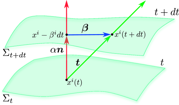
where we have defined . From the last equality in expression (27) it follows that and we will select , such that the associated vector field is future directed. The quantity is commonly referred to as the lapse function, it measures the rate of change of the coordinate time along the vector (see Fig. 1), and will be a building block of the metric in a 3+1 decomposition [cf., Eq. (37)].
The specification of the normal vector allows us to define the metric associated to each hypersurface, i.e.,
| (28) |
where , , but in general . Also note that , that is, and are the inverse of each other, so that the spatial metric can be used for raising and lowering the indices of purely spatial vectors and tensors.
The tensors and provide us with two useful tools to decompose any four-dimensional tensor into a purely spatial part (hence contained in the hypersurface ) and a purely timelike part (hence orthogonal to and aligned with ). Not surprisingly, the spatial part is readily obtained after contracting with the spatial projection operator (or spatial projection tensor)
| (29) |
while the timelike part is obtained after contracting with the time projection operator (or time projection tensor)
| (30) |
and where the two projectors are obviously orthogonal, i.e.,
| (31) |
Hence, a generic four-vector can be decomposed as
| (32) |
where the purely spatial part is still a four-vector that, by construction, has a zero contravariant time component, i.e., , whereas it has the covariant time component, , which is nonzero in general. Analogous considerations can be done about tensors of any rank.
We have already seen in Eq. (26) that the unit normal to a spacelike hypersurface does not represent the direction along which the time coordinate changes, that is, it is not the direction of the time derivative. Indeed, if we compute the contraction of the two tensors we obtain
| (33) |
We can therefore introduce a new vector, , along which to carry out the time evolutions and that is dual to the surface one-form . Such a vector is just the time-coordinate basis vector and is defined as the linear superposition of a purely temporal part (parallel to ) and of a purely spatial one (orthogonal to ), namely
| (34) |
The purely spatial vector [i.e., ] is usually referred to as the shift vector and will be another building block of the metric in a 3+1 decomposition [cf., Eq. (37)]. The decomposition of the vector into a timelike component and a spatial component is shown in Fig. 1 (note that in special relativity).
We can check that is a coordinate basis vector by verifying that
| (35) |
from which it follows that the vector is effectively dual to the one-form . This guarantees that the integral curves of are naturally parameterized by the time coordinate. As a result, all infinitesimal vectors originating on one hypersurface would end up on the same hypersurface . Note that this is not guaranteed for translations along and that since , the vector is not necessarily timelike (the shift can in fact be superluminal).
Using the components of
| (36) |
we can now express the generic line element in a 3+1 decomposition as
| (37) |
Expression (37) clearly emphasises that when , the lapse measures the proper time, , between two adjacent hypersurfaces, i.e.,
| (38) |
while the shift vector measures the change of coordinates of a point from the hypersurface to the hypersurface , i.e.,
| (39) |
Similarly, the covariant and contravariant components of the metric (37) can be written explicitly as
| (46) |
from which it is easy to obtain an important identity which will be used extensively hereafter, i.e.,
| (47) |
where and .
When defining the unit timelike normal in Eq. (27), we have mentioned that it can be associated to the four-velocity of a special class of observers, which are referred to as normal or Eulerian observers. Although this denomination is somewhat confusing, since such observers are not at rest with respect to infinity but have a coordinate velocity , we will adopt this traditional nomenclature also in the following and thus take an “Eulerian observer” as one with four-velocity given by (36).
When considering a fluid with four-velocity , the spatial four-velocity measured by an Eulerian observer will be given by the ratio between the projection of in the space orthogonal to , i.e., , and the Lorentz factor of as measured by deFelice90
| (48) |
As a result, the spatial four-velocity of a fluid as measured by an Eulerian observer will be given by
| (49) |
or, in component form, by
| (50) | ||||||
| (51) |
Using now the normalisation condition and indicating as usual with the Lorentz factor, we obtain
| (52) |
so that the components (50)–(51) can finally, be written as
| (53) |
where in the last equality we have exploited the fact that . Finally, using expressions (49) and (52), it is also possible to write the fluid four-velocity as
| (54) |
which highlights the split of into a temporal and a spatial part.
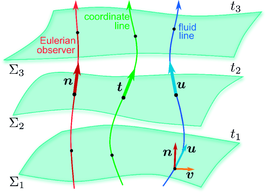
The three different unit four-vectors in a 3+1 decomposition of spacetime are shown in Fig. 2, which should be compared with Fig. 1. The four-vectors , and represent the unit timelike normal, the time-coordinate basis vector and the fluid four-velocity, respectively. Also shown are the associated worldlines, namely, the normal line representing the worldline of an Eulerian observer, the coordinate line representing the worldline of a coordinate element, and the fluidline. The figure also reports the spatial projection of the fluid four-velocity , thus highlighting that is the three-velocity as measured by the normal observer.
What remains to be done at this point is to apply the 3+1 decomposition to the relevant vector fields that appear in the GRMHD equations. In particular, we start by expressing the Faraday tensor and the dual of the Faraday tensor in Maxwell’s equations (9) and (10) respectively as
| (55) | ||||
| (56) |
where the spatial components of the electric and magnetic fields measured by the Eulerian observer are given as
| (57) |
We should note that our definition of the electric and magnetic fields differs by a factor from the corresponding definition used in Refs. Komissarov1999 ; Gammie03 .
Going back to the definition of the total current density (25) and recalling that the conduction current is purely spatial, i.e., , we can express its spatial components in terms of what is otherwise referred to as Ohm’s law Palenzuela:2008sf ; Bucciantini2012a ,
| (58) |
where is the resistivity and is the inverse of the scalar term of the conductivity tensor, i.e., Harutyunyan2018 , where is a Levi-Civita antisymmetric symbol, and where we have ignored the Hall or dynamo terms for simplicity (see Refs. Bucciantini2012a ; Palenzuela:2008sf where these terms are included in a generalized Ohm’s law). Assuming now the ideal MHD condition expressed by Eq. (14), we can obtain the explicit and algebraic expression between the electric and magnetic fields
| (59) |
This results, which coincides with the equivalent expression in Newtonian MHD, underlines the passive role of dependent quantity for the electric field in the ideal-MHD equations.
Finally, using Eq. (20) together with (57), we can obtain the transformation between magnetic four-vector field in the fluid frame and the magnetic four-vector field in the Eulerian frame as
| (60) |
which allows us to express the dual Faraday tensor (20) in terms of the magnetic four-vector field in the Eulerian frame as
| (61) |
and calculate the scalar as
| (62) |
where .
0.4 Formulation of the GRMHD equations for numerical simulations
0.4.1 Conservative Formulations
The equations of (relativistic) hydrodynamics and MHD can be written in the generic first-order-in-time form
| (63) |
and the system above is said to be hyperbolic if the matrix of coefficients is diagonalisable with a set of real eigenvalues, or eigenspeeds, and a corresponding set of linearly independent right eigenvectors , such that , is the diagonal matrix of eigenvalues and the matrix of right eigenvectors.
The most important property of hyperbolic equations is that they are well-posed, hence suitable for numerical solution. Moreover, if the matrix is the Jacobian of a flux vector with respect to the state vector , namely if , then the homogeneous version of the system (63) can be written in conservative form as
| (64) |
where is therefore called the vector of conserved variables. With this definition in mind, we can now discuss two theorems underlining the importance of a conservative formulation. The first one loosely speaking states that: conservative numerical schemes, – that is, a numerical scheme based on the conservative formulation of the equations – if convergent, do converge to the weak solution of the problem Lax60 . The second theorem states instead that: non-conservative schemes, i.e., schemes in which the equations are not written in the conservative form (64), do not converge to the correct solution if a shock wave is present in the flow Hou94 . In other words, the two theorems above state that if a conservative formulation is used, then we are guaranteed that the numerical solution will converge to the correct one, while if a conservative formulation is not used, we are guaranteed to converge to the incorrect solution in the likely event in which the flow develops a discontinuity.
0.4.2 The 3+1 Valencia formulation(s)
Given the importance of a conservative formulation to obtain a well-posed system of equations, more than 30 years ago the group of Valencia started to develop Eulerian 3+1 formulations of the relativistic hydrodynamic and MHD equations written in conservative forms. Because of this, these formulations are often referred to as the “Valencia formulations”. The first step in this direction was taken by considering the equations of special-relativistic hydrodynamics, which were cast into a conservative formulation Marti91 and solved in conjunction with High-Resolution Shock-Capturing (HRSC) methods (see, e.g., Rezzolla_book:2013 for an introduction to HRSC methods). The second step was taken a few years later, when the equations of genera-relativistic hydrodynamics were cast into a conservative formulation Banyuls97 and have been employed in a variety of numerical simulations starting from Refs. Font02c ; Baiotti04 . A final step, which is very relevant to the content of this chapter, was taken when the equations of GRMHD were cast in an Eulerian conservative formulation Anton06 .
In what follows, we detail the steps that are needed in order to cast the covariant set ideal-GRMHD equations (1), (2), (9), (10) into the following 3+1 and Eulerian conservative form
| (65) |
where is the vector of conserved variables, are the flux vectors (or “fluxes”), and is the vector of source terms.
We can start from the covariant continuity equation (1), which can be written as
| (66) |
which, after introducing the conserved rest-mass density in the Eulerian frame,
| (67) |
can be rewritten in the conservative form
| (68) |
Equivalently, after defining the transport velocity , Eq. (68) can be further rewritten as
| (69) |
which represents the 3+1 conservative form of the continuity equation in a generic (curved) spacetime.
Before considering the 3+1 conservative form of the energy-momentum equations, it is useful to write the energy-momentum tensor in terms of quantities measured by the Eulerian observer. In particular, we can define the conserved total energy density as the full projection of the energy-momentum tensor along the unit normal to the spatial hypersurface , i.e.,
| (70) |
Similarly, the three-momentum density measured by the Eulerian observer is defined as the mixed parallel-transverse component of the energy-momentum tensor
| (71) |
while the purely spatial part of the energy-momentum tensor is given by
| (72) |
The corresponding four-dimensional definitions are given respectively by
| (73) |
and allow us to rewrite the energy-momentum tensor in its generic 3+1 decomposition
| (74) |
Next, recalling that the four-divergence of a symmetric rank-2 tensor is given by
| (75) |
we can express the conservation of energy-momentum tensor (2) as
| (76) |
and thus, using expression (74), obtain the 3+1 conservative form of the momentum-conservation equation in a curved spacetime
| (77) |
In a similar way, we can combine Eqs. (2) and (4) as
| (78) |
and replacing with its decomposed form (74) so that, after some algebra, we obtain the 3+1 conservative form of the energy-conservation equation in curved spacetime
| (79) |
Equations (77) and (79) both involve source terms on their right-hand sides. In particular, the source term of the momentum-conservation equation (77) can be written more explicitly as
| (80) |
where we have used the following identities
| (81) |
and
| (82) |
where are the Christoffel symbols. Similarly, the source terms of the energy-conservation equation (79) can be expressed explicitly as
| (83) |
where is the extrinsic curvature Alcubierre:2008 ; Gourgoulhon2012 ; Rezzolla_book:2013 . Expression (83) can be further simplified if the spacetime is stationary, in which case the term reduces to
| (84) |
We should note that the expressions for the right-hand side of the energy and momentum conservation equations are due to Ref. DelZanna2007 and do not correspond to the ones originally presented in Ref. Banyuls97 , which expressed the four divergences of the energy-momentum tensor as
| (85) |
While this expression is mathematically equivalent to Eq. (75), it leads to more complex expressions for the right-hand sides when expressed in a 3+1 decomposition.
The final equation needed to complete the set of GRMHD equations in 3+1 conservative form is relative to the electromagnetic sector and, in particular, Faraday’s law of induction. Using Eq. (10) and the definition of the dual Faraday tensor, it is possible to rewrite Eq. (20) in the 3+1 equivalent form
| (86) |
or, using the transport velocity, as
| (87) |
Equation (87) is also known as the general-relativistic induction equation and highlights how the evolution of the magnetic field is directly related to the curl of the vector product of the three-velocity and of the magnetic field, as in Newtonian MHD. Once the magnetic field is known, the electric field follows trivially from Eq. (59).
At this point, it is possible to collect Eqs. (68), (77), (79), and (86), so as to build the state vector, the fluxes and the source vector and hence write the ideal-GRMHD equations in the conservative Valencia formulation (65) Anton06 . More specifically, after some simple algebra, it is not difficult to derive the following expressions for the state and flux vectors
| (88) |
while the source vector has components
| (89) |
We note that since the linear combination of a conserved variable is still a conserved variable, the state vector of conserved variables (88) is not unique and different codes implement different definitions. A particularly common choice is to replace the conserved total energy density with its equivalent
| (90) |
so that the corresponding state and flux vectors are given by
| (91) |
while the source terms are not changed. Obviously, expressions (88) and (91) are mathematically equivalent, but their numerical implementation has shown that the latter systematically leads to more accurate evolutions.
A few remarks before concluding this section. First, in stark contrast with what happens for the conservative formulation of the Newtonian MHD equations (i.e., when , , and ), in GRMHD (but already in general-relativistic hydrodynamics) the relation between the primitive variables, i.e., , , (or ), and , and the conserved variables, i.e., , , , and , is not analytic. In other words, the calculation of the primitive variables from the conserved one, i.e., what is normally referred to as the “primitive recovery” procedure, cannot be done analytically but requires the use of a multidimensional root-finding approach. The latter needs to be implemented at each numerical cell of the computational domain and can be particularly complex when tabulated equations of state are employed. Over the years, various algorithms have been developed to ensure an accurate, efficient, and stable primitive recovery, aiming at minimizing error accumulation during the matter evolution. For compactness, we will not discuss here the feature of such algorithms, but detailed discussions and comparisons of different algorithms have been studied in Refs. Siegel2018a ; Kastaun2021 ; Espino2022 ; Ng2023b with specific focus on their accuracy and robustness. Second, the set of evolution equations (65) does not include another important equation that needs to be solved together such a set and that represents one of the most important ones in the actual solution of the GRMHD equations, namely, the divergence-free condition (96). Also in this case, we will not discuss here the numerous numerical approaches that are possible to limit or prevent the growth of the violations of the divergence-free condition – from the divergence-cleaning methods, over to the evolution of the vector potential and up to the sophisticated constrained-transport methods – and refer the interested reader to Ref. Olivares2019 for a recent review of the various methods, and to the following chapters in this book. Finally, in the absence of gravity and thus in flat spacetimes, the corresponding form of the special relativistic MHD equations can be obtained trivially after setting , , and . The corresponding set of equations is widely employed in particle physics to simulate the dynamics of the collisions of heavy ions and some representative examples can be found in Refs. Inghirami18 ; Mayer2024 .
0.4.3 General-Relativistic Resistive MHD Equations
As mentioned in the Introduction, the electrical conductivity in astrophysical plasmas is extremely high and the ideal-MHD condition of infinite conductivity represents a very good approximation. In this case, the magnetic flux is conserved and the magnetic field is frozen in the fluid, being simply advected with it, and the electric field is trivially obtained from expression (59). By construction, therefore, the solution of the ideal-GRMHD equations neglects any effect of resistivity on the dynamics. In practice, however, even in astrophysical plasmas there will be spatial regions with very high temperatures where the electrical conductivity is finite and the resistive effects, most notably, the creation of current sheets and the consequent reconnection, will play a role. Such effects are expected to take place, for example, during the merger of two magnetized neutron stars or in accretion disks onto supermassive black holes, and could provide an important contribution to the energy losses from the system.
In all of these scenarios, the ideal-MHD limit may not be sufficient to study those physical processes that involve reconnection or the presence of anisotropic resistivities. This has motivated the derivation of a more extended set of GRMHD equations that accounts for resistive effects and that, in practice is augmented by an evolution equation for the electric field and by an extended Ohm’s law. The corresponding system is normally referred to as the set of general-relativistic resistive MHD (GRRMHD) equations, and we refer to Ref. Palenzuela:2008sf , where this system was first presented.
Since the changes with respect to the GRMHD equations take place only in the electromagnetic sector, the conservation equations of rest-mass (68), momentum (77), and energy (79) remain unchanged. On the other hand, the terms involved in the basic decomposition of the energy-momentum tensor (74) are modified because of the explicitly appearance of the electric fields and take the form
| (92) | ||||
| (93) | ||||
| (94) |
The new expressions for the electromagnetic sector involve the evolution equation for the magnetic field (10) (Faraday’s induction law), whose modified expression takes into account also the contributions from the electric fields
| (95) |
and the corresponding divergence-free constraint following from the temporal component of Eq. (10)
| (96) |
In addition, Ampere’s law for the evolution of the electric field follows from the spatial part of the second couple of Maxwell equations (10) and is given by
| (97) |
while the temporal component of (10) expresses the charge density in terms of the divergence of the electric field, i.e.,
| (98) |
Substituting now Eqs. (58) and (98) in Ampere’s law (97), we can rewrite it as
| (99) |
At this point, we can finally collect Eqs. (68), (77), (79), (95), and (97), so as to obtain the conservative form (65) of the GRRMHD equations. The corresponding augmented state and flux vectors are given by
| (100) |
while the source terms are
| (101) |
Note that, as for the set of GRMHD equations, also the set of GRRMHD equations is not closed and requires the specification of an equation of state. Similarly, a complex primitive-recovery approach is needed to compute at each numerical cell the primitive variables from the conserved ones (see, e.g., Ref. Ripperda2019 ). What is new, however, is that Ohm’s law (58) does not provide any information on the properties of the resistivity, which will in general be a function of space and time, i.e., . In principle, the information about the properties of the resistivity should follow from microphysical considerations and hence be calculated under specific physical conditions (see, e.g., Harutyunyan2018 in the case of neutron-star matter). In practice, however, given the poor knowledge of the resistive aspects of astrophysical plasmas, much cruder choices are made that model the resistivity as a constant or as a simple function of the rest-mass density (see, e.g., Dionysopoulou:2012pp ; Palenzuela2013 ). Finally, it should be mentioned that the solution of the GRRMHD equations is considerably more challenging that those of the GRMHD equations. For the former set, in fact, the equations become mixed hyperbolic-parabolic in Newtonian physics or hyperbolic with stiff relaxation terms in special relativity. The appearance of stiff terms in the equations follows from the fact that the diffusive effects take place on timescales that are intrinsically larger than the dynamical one or, in other words, from the fact the relaxation terms dominate over the purely hyperbolic ones, posing severe constraints on the timestep for the evolution (similar difficulties arise when considering the inclusion of radiative effects; see, e.g., Refs. Zanotti2011 ; Radice2022 ; Musolino2023 ). Overall, the presence of stiff terms forces the use of specially designed numerical methods such as the implicit-explicit Runge-Kutta time-integration schemes or RK-IMEX pareschi_2005_ier , and hence a significant extension of the numerical infrastructure (see, e.g., Refs. Palenzuela2013 ; Ripperda2019 ).
0.5 Summary
The equations of MHD represent a very effective tool to describe the dynamics of astrophysical plasmas and because of this they are employed in a variety of scenarios in astrophysics and cosmology. When applied in their GRMHD form to study astrophysical compact objects, they are the most accurate and powerful tool to explore the properties of compact black holes and neutron stars in fully dynamical and nonlinear regimes. In this chapter, we have presented the MHD equations in generic and curved spacetimes, either in the ideal-MHD limit (GRMHD equations) or in the presence of resistivity (GRRMHD equations). We have also discussed the basic aspects of a 3+1 decomposition of spacetime and the importance of writing the MHD equations in a conservative form.
The purpose of this Chapter – together with Chapters 2, which covers the coupling of the MHD equations with the Einstein equations, and of Chapter 3, which reviews the properties of modern equations of state – is to lay out the mathematical foundations of the set of equations that will be employed extensively in the rest of the book and which have a more applied nature. In particular, after an introduction of some representative GRMHD codes in Part II, Part III and IV are dedicated to the study of the dynamics of a variety of astrophysical plasmas, either when the spacetime is held fixed because the plasmas are not self-gravitating (Part III) or when the spacetime is dynamically evolved because the plasmas are self-gravitating (Part IV).
Acknowledgements.
Y.M. is supported by the Shanghai Municipality orientation program of Basic Research for International Scientists (Grant No. 22JC1410600), the National Natural Science Foundation of China (Grant No. 12273022), and the National Key R&D Program of China (Grant No. 2023YFE0101200). L.R. is supported in part from the State of Hesse within the Research Cluster ELEMENTS (Project ID 500/10.006), by the ERC Advanced Grant “JETSET: Launching, propagation and emission of relativistic jets from binary mergers and across mass scales” (Grant No. 884631), and by the Walter Greiner Gesellschaft zur Förderung der physikalischen Grundlagenforschung e.V. through the Carl W. Fueck Laureatus Chair.References
- [1] Miguel Alcubierre. Introduction to Numerical Relativity. Oxford University Press, Oxford, UK, 2008.
- [2] D. Alic, P. Moesta, L. Rezzolla, O. Zanotti, and J. L. Jaramillo. Accurate Simulations of Binary Black Hole Mergers in Force-free Electrodynamics. Astrophys. J., 754:36, July 2012.
- [3] M. Anderson, E. W. Hirschmann, L. Lehner, S. L. Liebling, P. M. Motl, D. Neilsen, C. Palenzuela, and J. E. Tohline. Magnetized Neutron-Star Mergers and Gravitational-Wave Signals. Phys. Rev. Lett., 100(19):191101, May 2008.
- [4] M. Anderson, E. W. Hirschmann, S. L. Liebling, and D. Neilsen. Relativistic MHD with adaptive mesh refinement. Class. Quantum Grav., 23:6503–6524, November 2006.
- [5] A. M. Anile. Relativistic Fluids and Magneto-fluids. Cambridge University Press, Cambridge, UK, February 1990.
- [6] Peter Anninos, P. Chris Fragile, and Jay D Salmonson. Cosmos++: Relativistic magnetohydrodynamics on unstructured grids with local adaptive refinement. Astrophys. J., 635:723, 2005.
- [7] L. Antón, O. Zanotti, J. A. Miralles, J. M. Martí, J. M. Ibáñez, J. A. Font, and J. A. Pons. Numerical 3+1 General Relativistic Magnetohydrodynamics: A Local Characteristic Approach. Astrophys. J., 637:296–312, January 2006.
- [8] L. Baiotti, I. Hawke, P. J. Montero, F. Löffler, L. Rezzolla, N. Stergioulas, J. A. Font, and E. Seidel. Three-dimensional relativistic simulations of rotating neutron-star collapse to a Kerr black hole. Phys. Rev. D, 71(2):024035, January 2005.
- [9] Dinshaw S. Balsara. Higher-order accurate space-time schemes for computational astrophysics—Part I: finite volume methods. Living Reviews in Computational Astrophysics, 3(1):2, December 2017.
- [10] F. Banyuls, J. A. Font, J. M. Ibáñez, J. M. Martí, and J. A. Miralles. Numerical 3+1 general-relativistic hydrodynamics: A local characteristic approach. Astrophys. J., 476:221, 1997.
- [11] D. Bégué, A. Pe’er, G. Q. Zhang, B. B. Zhang, and B. Pevzner. cuHARM: A New GPU-accelerated GRMHD Code and Its Application to ADAF Disks. Astrophys. J., Supp., 264(2):32, February 2023.
- [12] N. Bucciantini and L. Del Zanna. A fully covariant mean-field dynamo closure for numerical 3 + 1 resistive GRMHD. Mon. Not. R. Astron. Soc., 428:71–85, January 2013.
- [13] P. Cerdá-Durán, J. A. Font, L. Antón, and E. Müller. A new general relativistic magnetohydrodynamics code for dynamical spacetimes. Astron. Astrophys., 492:937–953, December 2008.
- [14] Mani Chandra, Francois Foucart, and Charles F. Gammie. grim: A Flexible, Conservative Scheme for Relativistic Fluid Theories. Astrophys. J., 837(1):92, March 2017.
- [15] Mani Chandra, Charles F. Gammie, Francois Foucart, and Eliot Quataert. An Extended Magnetohydrodynamics Model for Relativistic Weakly Collisional Plasmas. Astrophys. J., 810(2):162, September 2015.
- [16] Patrick Chi-Kit Cheong, Alan Tsz-Lok Lam, Harry Ho-Yin Ng, and Tjonnie Guang Feng Li. Gmunu: paralleled, grid-adaptive, general-relativistic magnetohydrodynamics in curvilinear geometries in dynamical space-times. Monthly Notices of the Royal Astronomical Society, 508(2):2279–2301, 09 2021.
- [17] Riccardo Ciolfi. The key role of magnetic fields in binary neutron star mergers. General Relativity and Gravitation, 52(6):59, June 2020.
- [18] Federico Cipolletta, Jay Vijay Kalinani, Bruno Giacomazzo, and Riccardo Ciolfi. Spritz: a new fully general-relativistic magnetohydrodynamic code. Class. Quant. Grav., 37(13):135010, 2020.
- [19] Alejandro Cruz-Osorio, Christian M. Fromm, Yosuke Mizuno, Antonios Nathanail, Ziri Younsi, Oliver Porth, Jordy Davelaar, Heino Falcke, Michael Kramer, and Luciano Rezzolla. State-of-the-art energetic and morphological modelling of the launching site of the M87 jet. Nature Astronomy, 6:103–108, January 2022.
- [20] F. de Felice and C. J. S. Clarke. Relativity on curved manifolds. Cambridge University Press, 1990.
- [21] J.-P. De Villiers and J. F. Hawley. A Numerical Method for General Relativistic Magnetohydrodynamics. Astrophys. J., 589:458–480, May 2003.
- [22] L. Del Zanna and N. Bucciantini. Covariant and 3 + 1 equations for dynamo-chiral general relativistic magnetohydrodynamics. Mon. Not. R. Astron. Soc., 479(1):657–666, September 2018.
- [23] L. Del Zanna, O. Zanotti, N. Bucciantini, and P. Londrillo. ECHO: a Eulerian conservative high-order scheme for general relativistic magnetohydrodynamics and magnetodynamics. Astron. Astrophys., 473:11–30, October 2007.
- [24] K. Dionysopoulou, D. Alic, C. Palenzuela, L. Rezzolla, and B. Giacomazzo. General-relativistic resistive magnetohydrodynamics in three dimensions: Formulation and tests. Phys. Rev. D, 88(4):044020, August 2013.
- [25] K. Dionysopoulou, D. Alic, C. Palenzuela, L. Rezzolla, and B. Giacomazzo. General-relativistic resistive magnetohydrodynamics in three dimensions: Formulation and tests. Phys. Rev. D, 88(4):044020, August 2013.
- [26] M. D. Duez, Y. T. Liu, S. L. Shapiro, and B. C. Stephens. Relativistic magnetohydrodynamics in dynamical spacetimes: Numerical methods and tests. Phys. Rev. D, 72(2):024028, July 2005.
- [27] Pedro Luis Espino, Gabriele Bozzola, and Vasileios Paschalidis. Quantifying uncertainties in general relativistic magnetohydrodynamic codes. arXiv e-prints, pages arXiv–2210, 2022.
- [28] Z. B. Etienne, V. Paschalidis, R. Haas, P. Mösta, and S. L. Shapiro. IllinoisGRMHD: an open-source, user-friendly GRMHD code for dynamical spacetimes. Class. Quantum Grav., 32(17):175009, September 2015.
- [29] J. A. Font. Numerical hydrodynamics in general relativity. Living Rev. Relativ., 6:4, 2003.
- [30] J. A. Font, T. Goodale, S. Iyer, M. Miller, L. Rezzolla, E. Seidel, N. Stergioulas, W.-M. Suen, and M. Tobias. Three-dimensional numerical general relativistic hydrodynamics. II. Long-term dynamics of single relativistic stars. Phys. Rev. D, 65(8):084024, April 2002.
- [31] Charles F. Gammie, Jonathan C. McKinney, and Gábor Tóth. HARM: A Numerical Scheme for General Relativistic Magnetohydrodynamics. Astrophys. J., 589(1):444–457, May 2003.
- [32] B. Giacomazzo and L. Rezzolla. WhiskyMHD: a new numerical code for general relativistic magnetohydrodynamics. Class. Quantum Grav., 24:235, June 2007.
- [33] Bruno Giacomazzo and Luciano Rezzolla. The Exact Solution of the Riemann Problem in Relativistic MHD. Journal of Fluid Mechanics, 562:223–259, 2006.
- [34] Ore Gottlieb, Serena Moseley, Teresita Ramirez-Aguilar, Ariadna Murguia-Berthier, Matthew Liska, and Alexander Tchekhovskoy. On the Jet-Ejecta Interaction in 3D GRMHD Simulations of a Binary Neutron Star Merger Aftermath. Astrophys. J. Lett., 933(1):L2, July 2022.
- [35] Eric Gourgoulhon. 3+1 Formalism in General Relativity, volume 846 of Lecture Notes in Physics, Berlin Springer Verlag. Springer, 2012.
- [36] Arus Harutyunyan, Antonios Nathanail, Luciano Rezzolla, and Armen Sedrakian. Electrical resistivity and Hall effect in binary neutron star mergers. European Physical Journal A, 54(11):191, November 2018.
- [37] J. F. Hawley, L. L. Smarr, and J. R. Wilson. A numerical study of nonspherical black hole accretion. I Equations and test problems. Astrophys. J., 277:296–311, February 1984.
- [38] T. Y. Hou and P. G. LeFloch. Why Nonconservative Schemes Converge to Wrong Solutions: Error Analysis. Math. Comp., 62:497–530, 1994.
- [39] G. Inghirami, L. Del Zanna, A. Beraudo, M. Haddadi Moghaddam, F. Becattini, and M. Bleicher. Magneto-hydrodynamic simulations of Heavy Ion Collisions with ECHO-QGP. In Journal of Physics Conference Series, volume 1024 of Journal of Physics Conference Series, page 012043, May 2018.
- [40] Wolfgang Kastaun, Jay Vijay Kalinani, and Riccardo Ciolfi. Robust recovery of primitive variables in relativistic ideal magnetohydrodynamics. Physical Review D, 103(2):023018, 2021.
- [41] K. Kiuchi, Y. Sekiguchi, K. Kyutoku, M. Shibata, K. Taniguchi, and T. Wada. High resolution magnetohydrodynamic simulation of black hole-neutron star merger: Mass ejection and short gamma ray bursts. Phys. Rev. D, 92(6):064034, September 2015.
- [42] S. S. Komissarov. A Godunov-type scheme for relativistic magnetohydrodynamics. Mon. Not. R. Astron. Soc., 303:343–366, February 1999.
- [43] S. Koide D.L. Meier K. Shibata T. Kudoh. General relativistic simulation of early jet formation in a rapidly rotating black hole magnetosphere. Astrophys. J, 536:668–674, 2000.
- [44] P. D. Lax and B. Wendroff. Systems of conservation laws. Commun. Pure Appl. Math., 13:217–237, 1960.
- [45] R. J. Leveque. Finite Volume Methods for Hyperbolic Problems. Cambridge University Press, New York, 2002.
- [46] M Liska, C Hesp, A Tchekhovskoy, A Ingram, M van der Klis, and S Markoff. Formation of precessing jets by tilted black hole discs in 3d general relativistic mhd simulations. Mon. Not. R. Astron. Soc., 474(1):L81–L85, 2018.
- [47] Matthew Liska, Koushik Chatterjee, Alexand er Tchekhovskoy, Doosoo Yoon, David van Eijnatten, Casper Hesp, Sera Markoff, Adam Ingram, and Michiel van der Klis. H-AMR: A New GPU-accelerated GRMHD Code for Exascale Computing With 3D Adaptive Mesh Refinement and Local Adaptive Time-stepping. arXiv e-prints, page arXiv:1912.10192, December 2019.
- [48] Yuk Tung Liu, Stuart L. Shapiro, Zachariah B. Etienne, and Keisuke Taniguchi. General relativistic simulations of magnetized binary neutron star mergers. Phys. Rev. D, 78:024012, 2008.
- [49] J. M. Martí, J. M. Ibáñez, and J. A. Miralles. Numerical relativistic hydrodynamics: Local characteristic approach. Phys. Rev. D, 43:3794, 1991.
- [50] J. M. Martí and E. Müller. Grid-based Methods in Relativistic Hydrodynamics and Magnetohydrodynamics. Living Reviews in Computational Astrophysics, 1, December 2015.
- [51] Markus Mayer, Luciano Rezzolla, Hannah Elfner, Gabriele Inghirami, and Dirk H. Rischke. BHAC-QGP: three-dimensional MHD simulations of relativistic heavy-ion collisions, II. Application to Au-Au collisions. arXiv e-prints, page arXiv:2403.08669, March 2024.
- [52] J. C. McKinney. General relativistic magnetohydrodynamic simulations of the jet formation and large-scale propagation from black hole accretion systems. Mon. Not. R. Astron. Soc., 368:1561–1582, June 2006.
- [53] J. C. McKinney, A. Tchekhovskoy, A. Sadowski, and R. Narayan. Three-dimensional general relativistic radiation magnetohydrodynamical simulation of super-Eddington accretion, using a new code HARMRAD with M1 closure. Mon. Not. R. Astron. Soc., 441:3177–3208, July 2014.
- [54] Charles W. Misner, Kip S. Thorne, and John A. Wheeler. Gravitation. W. H. Freeman, San Francisco, 1973.
- [55] Y. Mizuno, K.-I. Nishikawa, S. Koide, P. Hardee, and G. J. Fishman. RAISHIN: A High-Resolution Three-Dimensional General Relativistic Magnetohydrodynamics Code. ArXiv Astrophysics e-prints, August 2006.
- [56] Y. Mizuno, S. Yamada, S. Koide, and K. Shibata. General relativistic magnetohydrodynamic simulations of collapsars: Rotating black hole cases. Astrophys. J., 606:395, 2004.
- [57] Yosuke Mizuno, Ziri Younsi, Christian M. Fromm, Oliver Porth, Mariafelicia De Laurentis, Hector Olivares, Heino Falcke, Michael Kramer, and Luciano Rezzolla. The current ability to test theories of gravity with black hole shadows. Nature Astronomy, 2:585–590, April 2018.
- [58] A. Murguia-Berthier, E. Ramirez-Ruiz, G. Montes, F. De Colle, L. Rezzolla, S. Rosswog, K. Takami, A. Perego, and W. H. Lee. The Properties of Short Gamma-Ray Burst Jets Triggered by Neutron Star Mergers. Astrophys. J. Lett., 835:L34, February 2016.
- [59] Carlo Musolino and Luciano Rezzolla. A practical guide to a moment approach for neutrino transport in numerical relativity. arXiv e-prints, page arXiv:2304.09168, April 2023.
- [60] R. Narayan, A. Sa̧dowski, R. F. Penna, and A. K. Kulkarni. GRMHD simulations of magnetized advection-dominated accretion on a non-spinning black hole: role of outflows. Mon. Not. R. Astron. Soc., 426:3241–3259, November 2012.
- [61] Antonios Nathanail, Ramandeep Gill, Oliver Porth, Christian M. Fromm, and Luciano Rezzolla. On the opening angle of magnetized jets from neutron-star mergers: the case of GRB170817A. Mon. Not. R. Astron. Soc., 495(4):3780–3787, May 2020.
- [62] Antonios Nathanail, Ramandeep Gill, Oliver Porth, Christian M. Fromm, and Luciano Rezzolla. 3D magnetized jet break-out from neutron-star binary merger ejecta: afterglow emission from the jet and the ejecta. Mon. Not. R. Astron. Soc., 502(2):1843–1855, April 2021.
- [63] Harry Ho-Yin Ng, Jin-Liang Jiang, Carlo Musolino, Christian Ecker, Samuel D. Tootle, and Luciano Rezzolla. Hybrid approach to long-term binary neutron-star simulations. Phys. Rev. D, 109(6):064061, March 2024.
- [64] Hector Olivares, Oliver Porth, Jordy Davelaar, Elias R. Most, Christian M. Fromm, Yosuke Mizuno, Ziri Younsi, and Luciano Rezzolla. Constrained transport and adaptive mesh refinement in the Black Hole Accretion Code. Astron. Astrophys., 629:A61, September 2019.
- [65] C. Palenzuela. Modelling magnetized neutron stars using resistive magnetohydrodynamics. Mon. Not. R. Astron. Soc., 431:1853–1865, May 2013.
- [66] C. Palenzuela, T. Garrett, L. Lehner, and S. L. Liebling. Magnetospheres of black hole systems in force-free plasma. Phys. Rev. D, 82(4):044045, August 2010.
- [67] C. Palenzuela, L. Lehner, M. Ponce, S. L. Liebling, M. Anderson, D. Neilsen, and P. Motl. Electromagnetic and Gravitational Outputs from Binary-Neutron-Star Coalescence. Phys. Rev. Lett., 111(6):061105, August 2013.
- [68] C. Palenzuela, L. Lehner, O. Reula, and L. Rezzolla. Beyond ideal MHD: towards a more realistic modelling of relativistic astrophysical plasmas. Mon. Not. R. Astron. Soc., 394:1727–1740, April 2009.
- [69] Lorenzo Pareschi and Giovanni Russo. Implicit–explicit runge–kutta schemes and applications to hyperbolic systems with relaxation. Journal of Scientific Computing, 25(1):129, 2005.
- [70] O. Porth, H. Olivares, Y. Mizuno, Z. Younsi, L. Rezzolla, M. Moscibrodzka, H. Falcke, and M. Kramer. The black hole accretion code. Computational Astrophysics and Cosmology, 4:1, May 2017.
- [71] Shi Pu, Victor Roy, Luciano Rezzolla, and Dirk H. Rischke. Bjorken flow in one-dimensional relativistic magnetohydrodynamics with magnetization. Phys. Rev. D, 93(7):074022, April 2016.
- [72] Q. Qian, C. Fendt, S. Noble, and M. Bugli. rHARM: Accretion and Ejection in Resistive GR-MHD. Astrophys. J., 834:29, January 2017.
- [73] David Radice, Sebastiano Bernuzzi, Albino Perego, and Roland Haas. A new moment-based general-relativistic neutrino-radiation transport code: Methods and first applications to neutron star mergers. Mon. Not. Roy. Astron. Soc., 512(1):1499–1521, 2022.
- [74] S. M. Ressler, A. Tchekhovskoy, E. Quataert, M. Chand ra, and C. F. Gammie. Electron thermodynamics in GRMHD simulations of low-luminosity black hole accretion. Mon. Not. R. Astron. Soc., 454(2):1848–1870, December 2015.
- [75] L. Rezzolla, B. Giacomazzo, L. Baiotti, J. Granot, C. Kouveliotou, and M. A. Aloy. The Missing Link: Merging Neutron Stars Naturally Produce Jet-like Structures and Can Power Short Gamma-ray Bursts. Astrophys. J. Letters, 732:L6, May 2011.
- [76] L. Rezzolla and K. Takami. Black-hole production from ultrarelativistic collisions. Class. Quantum Grav., 30(1):012001, January 2013.
- [77] L. Rezzolla and O. Zanotti. Relativistic Hydrodynamics. Oxford University Press, Oxford, UK, 2013.
- [78] B. Ripperda, F. Bacchini, O. Porth, E. R. Most, H. Olivares, A. Nathanail, L. Rezzolla, J. Teunissen, and R. Keppens. General-relativistic Resistive Magnetohydrodynamics with Robust Primitive-variable Recovery for Accretion Disk Simulations. Astrophys. J., Supp., 244(1):10, September 2019.
- [79] Victor Roy, Shi Pu, Luciano Rezzolla, and Dirk Rischke. Analytic Bjorken flow in one-dimensional relativistic magnetohydrodynamics. Physics Letters B, 750:45–52, November 2015.
- [80] A. Sa̧dowski, R. Narayan, A. Tchekhovskoy, and Y. Zhu. Semi-implicit scheme for treating radiation under M1 closure in general relativistic conservative fluid dynamics codes. Mon. Not. R. Astron. Soc., 429:3533–3550, March 2013.
- [81] M. Shibata and Y.-I. Sekiguchi. Magnetohydrodynamics in full general relativity: Formulation and tests. Phys. Rev. D, 72(4):044014, August 2005.
- [82] Daniel M. Siegel, Philipp Mösta, Dhruv Desai, and Samantha Wu. Recovery Schemes for Primitive Variables in General-relativistic Magnetohydrodynamics. Astrophys. J., 859(1):71, May 2018.
- [83] James M. Stone, Kengo Tomida, Christopher J. White, and Kyle G. Felker. The Athena++ Adaptive Mesh Refinement Framework: Design and Magnetohydrodynamic Solvers. Astrophys. J., Supp., 249(1):4, July 2020.
- [84] H. R. Takahashi, K. Ohsuga, T. Kawashima, and Y. Sekiguchi. Formation of Overheated Regions and Truncated Disks around Black Holes: Three-dimensional General Relativistic Radiation-magnetohydrodynamics Simulations. Astrophys. J., 826:23, July 2016.
- [85] A. Tchekhovskoy, R. Narayan, and J. C. McKinney. Efficient generation of jets from magnetically arrested accretion on a rapidly spinning black hole. Mon. Not. R. Astron. Soc., 418:L79–L83, November 2011.
- [86] E. F. Toro. Riemann Solvers and Numerical Methods for Fluid Dynamics. Springer-Verlag, third edition, 2009.
- [87] J. P. De Villiers and J. F. Hawley. Global general relativistic magnetohydrodynamic simulations of accretion tori. Astrophys. J., 592:1060, 2003.
- [88] C. J. White, J. M. Stone, and C. F. Gammie. An Extension of the Athena++ Code Framework for GRMHD Based on Advanced Riemann Solvers and Staggered-mesh Constrained Transport. Astrophys. J.s, 225:22, August 2016.
- [89] Christopher J. White, Eliot Quataert, and Charles F. Gammie. The Structure of Radiatively Inefficient Black Hole Accretion Flows. Astrophys. J., 891(1):63, March 2020.
- [90] O. Zanotti and M. Dumbser. A high order special relativistic hydrodynamic and magnetohydrodynamic code with space-time adaptive mesh refinement. Computer Physics Communications, 188:110–127, March 2015.
- [91] O. Zanotti, C. Roedig, L. Rezzolla, and L. Del Zanna. General relativistic radiation hydrodynamics of accretion flows - I. Bondi-Hoyle accretion. Mon. Not. R. Astron. Soc., 417:2899–2915, November 2011.