Surfaces with concentric or parallel $K$-contours

Abstract.

Surfaces with concentric $K$-contours and parallel $K$-contours in Euclidean $3$-space are defined. Crucial examples are presented and characterization of them are given.

1. Introduction

The contours of the Gaussian curvature function $K$ on the graph surface

$$z=\frac{x}{x^{2}+y^{2}}$$ (1.1)

in the Euclidean $3$-space $({\mathbb{R}}^{3};x,y,z)$ map to concentric circles on the $xy$-plane by orthogonal projection, so it would be permissible to say that the surface (1.1) has weak symmetry in some sense. We will refer to this property by saying a surface has concentric $K$-contours. We can immediately note that helicoidal surfaces have the same property. (Here a helicoidal surface is, by definition, a surface in ${\mathbb{R}}^{3}$ which is invariant under a one-parameter group of rigid screw motions; it is a generalization of both surfaces of revolution and right helicoids. A helicoidal surface is also called a generalized helicoid (cf. [1])). We also found that the surface called a monkey saddle has the same property. (See Section 22.2 in [2], where the monkey saddle appears as an example for which the converse of Gauss’ Theorema Egregium does not hold.) In view of these circumstances, simple questions come to mind:

1. Are there any surfaces with concentric $K$-contours other than (1.1), helicoidal surfaces or the monkey saddle?

2. Can we find all surfaces with concentric $K$-contours?

The authors searched the literature, but failed to find research on this.

One of our purposes is to provide a family of examples, denoted by ${\boldsymbol{x}}_{m,c}$ in this paper, which includes both (1.1) and the monkey saddle. Another purpose is to give a partial answer to the question (ii). In fact, under a certain assumption, any surface with concentric $K$-contours must be a surface ${\boldsymbol{x}}_{m,c}$ or a helicoidal surface (Theorem 2.4).

On the other hand, it has been an interesting problem to understand how much the behavior of the Gauss map determines the surface. For instance, Kenmotsu [4] showed a representation theorem for an arbitrary surface in ${\mathbb{R}}^{3}$ in terms of the Gauss map and the mean curvature function of the surface. In addition to this, Hoffman, Osserman and Schoen [3] proved that for a complete oriented surface of constant mean curvature in ${\mathbb{R}}^{3}$, if its Gauss image lies in some open hemisphere, then it is a plane; if the Gauss image lies in a closed hemisphere, then it is a plane or a right circular cylinder. In this paper, we will show that a behavior of the Gauss map, called semi-rotational equivariance, characterizes the surfaces ${\boldsymbol{x}}_{m,c}$ (Theorem 2.5).

This paper also reports on the case where concentric circles are replaced by parallel straight lines. We say that a surface has parallel K-contours if the contours of the Gaussian curvature function $K$ produce parallel straight lines on a plane by orthogonal projection.

We refer to standard textbooks [1], [5], [6], etc, for fundamental facts about surface theory.

2. Surfaces with concentric $K$-contours

Throughout this paper, we shall use the following notation and assumption: $M$ denotes a connected, smooth $2$-manifold and ${\boldsymbol{x}}\colon M\to{\mathbb{R}}^{3}$ a smooth immersion. $K$ denotes the Gaussian curvature function on $M$. We set $M_{k}:=\{p\in M\mid K(p)=k\}$ for a real number $k$, and consider the family $\mathcal{C}:=\{M_{k}\}_{k\in{\mathbb{R}}}$. It is always assumed that $M$ has no open subset where $\operatorname{grad}K=0$ because we wish to study the case where $\mathcal{C}$ is formed by a family of curves.

Definition 2.1.

We say that ${\boldsymbol{x}}\colon M\to{\mathbb{R}}^{3}$ has concentric K-contours if there exists a plane in ${\mathbb{R}}^{3}$ such that the orthogonal projection $\pi\colon{\mathbb{R}}^{3}\to P$ maps $\mathcal{C}$ to a family of concentric circles on $P$.

It is obvious that helicoidal surfaces have concentric $K$-contours.

2.1. A non-helicoidal example

Let $m$ be an integer not equal to $0,1$, and let $c$ be a non-zero real number. Consider a graph surface

$${\boldsymbol{x}}_{m,c}(z)=\left(\operatorname{Re}z,\operatorname{Im}z,c\operatorname{Re}(z^{m})\right)=\left(x,y,\frac{c}{2}\left\{(x+iy)^{m}+(x-iy)^{m}\right\}\right)$$ (2.1)

for $z=x+iy$. Note that ${\boldsymbol{x}}_{-1,1}$ and ${\boldsymbol{x}}_{3,1}$ coincide with the surface (1.1) and the monkey saddle, respectively. In terms of the polar coordinates $z=re^{i\theta}$, ${\boldsymbol{x}}_{m,c}$ is expressed as

$${\boldsymbol{x}}_{m,c}(r,\theta)=\left(r\cos\theta,r\sin\theta,cr^{m}\cos m\theta\right).$$ (2.2)

See Figures 1 and 2.

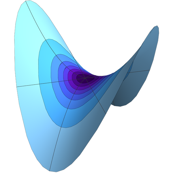
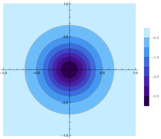
$c=1$, $m=2$
 
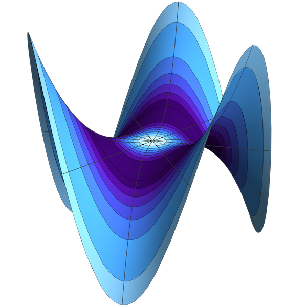
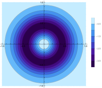
$c=1$, $m=3$

Figure 1. The surfaces ${\boldsymbol{x}}_{m,c}$ (left) and their projections to the $xy$-plane (right) with positive integers $m$. Each surface is gray-scaled by its Gaussian curvature.

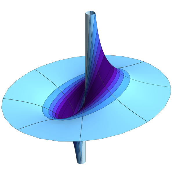
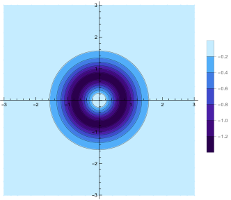
$c=1$, $m=-1$
 
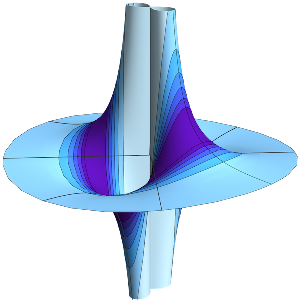
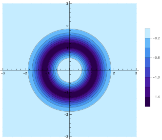
$c=1$, $m=-2$

Figure 2. The surfaces ${\boldsymbol{x}}_{m,c}$ (left) and their projections to the $xy$-plane (right) with negative integers $m$. Each surface is gray-scaled by its Gaussian curvature.

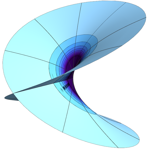
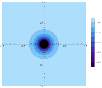
$c=1$, $m=1/2$
 
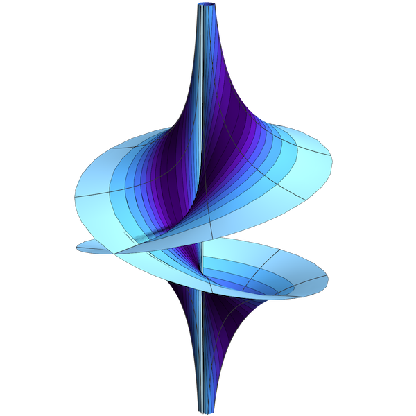
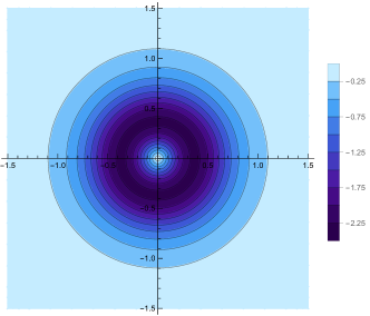
$c=1$, $m=-1/2$

Figure 3. The surfaces ${\boldsymbol{x}}_{m,c}$ (left) and their projections to the $xy$-plane (right) with non integers $m$. Each surface is gray-scaled by its Gaussian curvature.

The first and second fundamental forms $\,\mathrm{I},\,\mathrm{I\!I}$ and a unit normal $\boldsymbol{n}$ are as follows:

$$\begin{aligned} \,\mathrm{I}=&\,(1+c^{2}m^{2}r^{2m-2}\cos^{2}m\theta)dr^{2}+2(-c^{2}m^{2}r^{2m-1}\cos m\theta\sin m\theta)drd\theta\\ &+(r^{2}+c^{2}m^{2}r^{2m}\sin^{2}m\theta)d\theta^{2},\end{aligned}$$

$$\boldsymbol{n}(r,\theta)=\frac{1}{r\sqrt{1+c^{2}m^{2}r^{2m-2}}}\left(-cmr^{m}\cos(m-1)\theta,cmr^{m}\sin(m-1)\theta,r\right),$$ (2.3)

$$\,\mathrm{I\!I}=\frac{cm(m-1)}{r\sqrt{1+c^{2}m^{2}r^{2m-2}}}\left\{r^{m-1}\cos m\theta dr^{2}-2r^{m}\sin m\theta drd\theta-r^{m+1}\cos m\theta d\theta^{2}\right\}.$$

From these, the Gaussian curvature $K$ and the mean curvature $H$ are

$$K=K(r)=-\frac{c^{2}m^{2}(m-1)^{2}r^{2m-4}}{(1+c^{2}m^{2}r^{2m-2})^{2}},$$ (2.4)

$$H=H(r,\theta)=-\frac{c^{3}m^{3}(m-1)r^{3m-4}\cos m\theta}{2(1+c^{2}m^{2}r^{2m-2})^{3/2}}.$$

It follows directly from (2.4) that ${\boldsymbol{x}}_{m,c}$ has concentric $K$-contours with respect to the $xy$-plane. Note that the first fundamental form $\,\mathrm{I}$ does not have rotational symmetry but the Gaussian curvature $K$ does.

Remark 2.2.

1. It follows from (2.1) that ${\boldsymbol{x}}_{m,c}$ is an entire graph over the $xy$-plane if $m$ is a positive integer. In particular, ${\boldsymbol{x}}_{m,c}$ is a hyperbolic paraboloid if $m=2$ and a monkey saddle if $m=3$. In the case where $m$ is a negative integer, ${\boldsymbol{x}}_{m,c}$ is a graph punctured at the origin.

2. Although ${\boldsymbol{x}}_{m,c}$ can be defined for $m=0,1$ or $c=0$, it is a plane hence has constant Gaussian curvature zero. Therefore we exclude the case $m=0,1$ and the case $c=0$.

It follows from (2.2) that ${\boldsymbol{x}}_{m,c}$ can be defined even if $m$ is a non-integer as a multi-valued graph over ${\mathbb{R}}^{2}\setminus\{(0,0)\}$ or a surface defined on the universal cover. See Figure 3. From now on, we assume that the number $m$ for ${\boldsymbol{x}}_{m,c}$ does not have to be an integer, that is, $m\in{\mathbb{R}}\setminus\{0,1\}$.

2.2. Semi-rotational equivariance

We also call the unit normal (2.3) the Gauss map of ${\boldsymbol{x}}_{m,c}$ according to custom. One can see from (2.3) that

$$\boldsymbol{n}(r,\theta+\alpha)=\mathcal{R}_{(1-m)\alpha}\circ\boldsymbol{n}(r,\theta),$$

where $\mathcal{R}_{(1-m)\alpha}$ denotes the rotation of angle $(1-m)\alpha$ with respect to the $z$-axis. Focusing on this property, we give the following definition:

Definition 2.3.

A surface ${\boldsymbol{x}}\colon M\to{\mathbb{R}}^{3}$ is said to have semi-rotational Gauss map if there exist a straight line $l\subset{\mathbb{R}}^{3}$, a plane $P\subset{\mathbb{R}}^{3}$, and a $1$-parameter group $\{\phi_{t}\}$ of diffeomorphisms of $M$ such that

1. $l$ is orthogonal to $P$,

2. $\pi\circ{\boldsymbol{x}}\circ\phi_{t}=R_{t}\circ\pi\circ{\boldsymbol{x}}$, and

3. $\boldsymbol{n}\circ\phi_{t}=\mathcal{R}_{kt}\circ\boldsymbol{n}$ for some constant $k$

with a suitable choice of orientations of $l$ and $P$, where $\pi\colon{\mathbb{R}}^{3}\to P$ is orthogonal projection, $R_{t}$ denotes a rotation on $P$ of angle $t$ with the center $P\cap l$, and $\mathcal{R}_{kt}$ denotes a rotation in ${\mathbb{R}}^{3}$ of angle $kt$ with respect to the axis $l$.

Note that a helicoidal surface has semi-rotational Gauss map with $k=1$, which should be said to have rotational Gauss map. So we shall use the term ‘strictly semi-rotational’ in the sense of ‘semi-rotational but not rotational’.

2.3. Characterizations of the surface ${\boldsymbol{x}}_{m,c}$

Theorem 2.4.

Let ${\boldsymbol{x}}\colon M\to{\mathbb{R}}^{3}$ be a surface with concentric $K$-contours. If the area element $dA$ is invariant along each $K$-contour, then ${\boldsymbol{x}}$ is a helicoidal surface or locally congruent to a surface ${\boldsymbol{x}}_{m,c}$ for some $m,c$.

Theorem 2.5.

Let a surface ${\boldsymbol{x}}\colon M\to{\mathbb{R}}^{3}$ have semi-rotational Gauss map. Then ${\boldsymbol{x}}$ is a helicoidal surface or locally congruent to a surface ${\boldsymbol{x}}_{m,c}$ for some $m,c$.

Corollary 2.6.

Let a surface ${\boldsymbol{x}}\colon M\to{\mathbb{R}}^{3}$ have strictly semi-rotational Gauss map. Then ${\boldsymbol{x}}$ is locally congruent to a surface ${\boldsymbol{x}}_{m,c}$ for some $m,c$.

Before proving the theorems above, we write down formulas for the area element $dA$, the Gaussian curvature $K$ and the unit normal field $\boldsymbol{n}$ for a surface ${\boldsymbol{x}}(r,\theta)=\left(r\cos\theta,r\sin\theta,F(r,\theta)\right)$ :

$$dA =\varDelta\,dr\wedge d\theta,$$ (2.5)

$$\boldsymbol{n} =\frac{1}{\varDelta}\left(F_{\theta}\sin\theta-rF_{r}\cos\theta,\ -rF_{r}\sin\theta-F_{\theta}\cos\theta,\ r\right),$$ (2.6)

$$K =\frac{1}{\varDelta^{4}}\left\{r^{2}F_{rr}(rF_{r}+F_{\theta\theta})-(F_{\theta}-rF_{r\theta})^{2}\right\},$$ (2.7)

where

$$\varDelta=\sqrt{r^{2}+r^{2}F_{r}^{2}+F_{\theta}^{2}}.$$ (2.8)

Proof of Theorem 2.4.

Considering a rigid motion in ${\mathbb{R}}^{3}$, we may assume that the plane $P$ is the $xy$-plane and $K$-contours draw concentric circles with the center $(0,0)$ in the $xy$-plane. ${\boldsymbol{x}}$ is at least locally re-parameterized as ${\boldsymbol{x}}(r,\theta)=\left(r\cos\theta,r\sin\theta,F(r,\theta)\right)$. The function $\varDelta$ is of one variable $r$ because of (2.5) and the assumption of invariance of $dA$. It follows from (2.8) that $r^{2}F_{r}^{2}+F_{\theta}^{2}$ is also a function of one variable $r$. Therefore, there exist functions $\alpha=\alpha(r)$, $\beta=\beta(r,\theta)$ such that

$$rF_{r}=\alpha\cos\beta,\ F_{\theta}=\alpha\sin\beta.$$ (2.9)

By differentiating (2.9), we have

$$r^{2}F_{rr} =(r\alpha^{\prime}-\alpha)\cos\beta-r\alpha\beta_{r}\sin\beta,$$ (2.10)

$$r(F_{r})_{\theta} =-\alpha\sin\beta\cdot\beta_{\theta},$$ (2.11)

$$(F_{\theta})_{r} =\alpha^{\prime}\sin\beta+\alpha\cos\beta\cdot\beta_{r},$$ (2.12)

$$F_{\theta\theta} =\alpha\cos\beta\cdot\beta_{\theta}.$$ (2.13)

It follows from (2.11), (2.12) that the equality $(F_{r})_{\theta}=(F_{\theta})_{r}$ turns out to be

$$\frac{\beta_{\theta}}{r}+\beta_{r}\frac{\cos\beta}{\sin\beta}=-\frac{\alpha^{\prime}}{\alpha}.$$ (2.14)

Note that the right side of (2.14) is of one variable $r$, so the left side is as well. Thus

$$\frac{\partial}{\partial\theta}\left(\frac{\beta_{\theta}}{r}+\beta_{r}\frac{\cos\beta}{\sin\beta}\right)=0.$$ (2.15)

On the other hand, using (2.10)–(2.13), we can rewrite (2.7) as

$$K=\frac{\alpha(1+\beta_{\theta})(r\alpha^{\prime}-\alpha)}{\varDelta^{4}}.$$

Here, $K$ must be a non-constant function of one variable $r$ by the assumption of concentric $K$-contours. It implies that $\beta_{\theta}$ is a function of one variable $r$. Therefore, we may set $\beta_{\theta}=\phi(r)$ and hence

$$\beta=\phi(r)\cdot\theta+\psi(r)$$ (2.16)

for some functions $\phi(r)$, $\psi(r)$. It follows from (2.15) with (2.16) that

$$\phi^{\prime}(r)\{\frac{1}{2}\sin 2\beta-\phi(r)\cdot\theta\}+\psi^{\prime}(r)\phi(r)=0.$$

This implies that (i) $\frac{1}{2}\sin 2\beta-\phi(r)\cdot\theta$ is independent of $\theta$ or (ii) $\phi^{\prime}(r)=0$. In the case (i), by differentiating $\frac{1}{2}\sin 2\beta-\phi(r)\cdot\theta$ by $\theta$, we have $(\cos 2\beta-1)\phi(r)=0$, that is,

$$\beta=n\pi n \beta=\psi(r)$$ for some integer or . (2.17)

In the case (ii), the function $\phi$ is constant and $\psi^{\prime}\phi=0$. Therefore $(\phi,\psi)=(k,l)$ for some constants $k,l$ or $(\phi,\psi)=(0,\psi(r))$; in other words,

$$\beta=k\theta+l \beta=\psi(r)$$ or . (2.18)

Since the condition (2.18) includes the condition (2.17), we continue to discuss under the condition (2.18).

In the case where $\beta=k\theta+l$, the equation (2.14) reduces to $\alpha^{\prime}=-k\alpha/r$. Hence we have $\alpha=Cr^{-k}$ for some constant $C$. It follows from (2.9) that $F=C_{1}r^{k}\cos(k\theta+l)+C_{2}$ for some constants $C_{1},C_{2}$. Thus the surface ${\boldsymbol{x}}$ is congruent to ${\boldsymbol{x}}_{k,C_{1}}$.

In the case where $\beta=\psi(r)$, the equation (2.14) reduces to $\psi^{\prime}\cot\psi=\alpha^{\prime}/\alpha$. It is solved as $\alpha\sin\psi=C$ for some constant $C$. The system of equations (2.9) turns out to be

$$rF_{r}=\alpha(r)\cos(\psi(r)),\quad F_{\theta}=C.$$

Therefore, we obtain

$$F=C\theta+\int\frac{\alpha(r)}{r}\cos(\psi(r))dr=C\theta+A(r)$$

for some function $A(r)$. Thus the surface ${\boldsymbol{x}}$ is helicoidal. ∎

Proof of Theorem 2.5.

Considering a rigid motion in ${\mathbb{R}}^{3}$, we may assume that the plane $P$ is the $xy$-plane and the line $l$ is the $z$-axis. The surface ${\boldsymbol{x}}$ is at least locally re-parameterized as ${\boldsymbol{x}}(r,\theta)=\left(r\cos\theta,r\sin\theta,F(r,\theta)\right)$. The Gauss map (2.6) is

$$\boldsymbol{n}=\frac{1}{\varDelta}\begin{pmatrix}F_{\theta}\sin\theta-rF_{r}\cos\theta\\ -rF_{r}\sin\theta-F_{\theta}\cos\theta\\ r\end{pmatrix}=\begin{pmatrix}\cos\theta&-\sin\theta&0\\ \sin\theta&\cos\theta&0\\ 0&0&1\end{pmatrix}\frac{1}{\varDelta}\begin{pmatrix}-rF_{r}\\ -F_{\theta}\\ r\end{pmatrix}$$

in the column-vector form. Since $\boldsymbol{n}$ is semi-rotational,

1. the vector-valued function

   $$\dfrac{1}{\varDelta}\begin{pmatrix}-rF_{r},-F_{\theta},r\end{pmatrix}$$ (2.19)

   is of one variable $r$, or

2. there exist $m\in\mathbb{R}$ and $\phi_{1}=\phi_{1}(r),\psi=\psi(r)$ such that

   $$\frac{1}{\varDelta}\begin{pmatrix}-rF_{r},-F_{\theta},r\end{pmatrix}=\begin{pmatrix}\phi_{1}(r)\cos m\theta,\phi_{1}(r)\sin m\theta,\psi(r)\end{pmatrix}.$$

In the case (i), each component of (2.19) is of one variable $r$. Hence, $\varDelta$, $F_{r}$ and $F_{\theta}$ are functions of one variable $r$. This implies that $F$ must be of the form $F=a\theta+\psi(r)$ for a constant $a$ and a function $\psi(r)$. Therefore ${\boldsymbol{x}}(r,\theta)=\left(r\cos\theta,r\sin\theta,a\theta+\psi(r)\right)$, that is, ${\boldsymbol{x}}$ is a helicoidal surface.

In the case (ii), the third component of (2.19) is of one variable $r$. Hence, $\varDelta$ is a function of one variable $r$. Setting $-\phi_{1}(r)\cdot\varDelta=\varphi(r)$, we have

$$\begin{cases}F_{r}=\frac{\varphi(r)}{r}\cos m\theta\\ F_{\theta}=\varphi(r)\sin m\theta.\end{cases}$$ (2.20)

Thus the equality $(F_{r})_{\theta}=(F_{\theta})_{r}$ turns out to be

$$-m\frac{\varphi(r)}{r}\sin m\theta=\varphi^{\prime}(r)\sin m\theta.$$ (2.21)

In the case where $m=0$, the system of equations (2.20) turns out to be $F_{r}=\varphi(r)/r,F_{\theta}=0$. Therefore, $F=F(r)$. This implies that ${\boldsymbol{x}}$ is a rotational surface.

In the case where $m\neq 0$, the equation (2.21) leads to $-m\frac{\varphi(r)}{r}=\varphi^{\prime}(r)$. Therefore, $\varphi(r)=Cr^{-m}$ ($C$ is a constant.) Then the solution to the system of equations (2.20) is

$$F(r,\theta)=C_{1}r^{-m}\cos m\theta+C_{2}\quad\text{($C_{1},C_{2}$ are constants).}$$

Thus ${\boldsymbol{x}}$ is congruent to ${\boldsymbol{x}}_{-m,C_{1}}$. ∎

3. Surfaces with parallel $K$-contours

We shall discuss here using the same notations and assumption as in Section 2.

Definition 3.1.

We say that a surface ${\boldsymbol{x}}\colon M\to{\mathbb{R}}^{3}$ has parallel K-contours if there exists a plane in ${\mathbb{R}}^{3}$ such that the orthogonal projection $\pi\colon{\mathbb{R}}^{3}\to P$ maps $\mathcal{C}$ to a family of parallel straight lines on $P$.

3.1. An example

Let $k$, $c$ be non-zero real numbers. Consider a graph surface of

$$z=ce^{kx}\cos ky,$$

that is,

$$\boldsymbol{p}_{k,c}(x,y)=\left(x,y,ce^{kx}\cos ky\right).$$

See Figure 4.

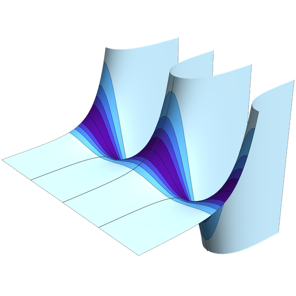
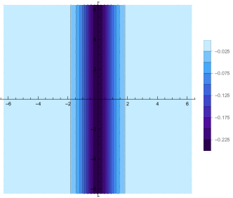
Figure 4. The surface $\boldsymbol{p}_{k,c}$ (left) and its projection to the $xy$-plane (right) for $c=1$ and $k=1$. The surface is gray-scaled by its Gaussian curvature.

The first and second fundamental forms $\,\mathrm{I},\,\mathrm{I\!I}$ and a unit normal $\boldsymbol{n}$ are as follows:

$$\begin{aligned} \,\mathrm{I}=\ &(1+c^{2}k^{2}e^{2kx}\cos^{2}ky)dx^{2}-2c^{2}k^{2}e^{2kx}\cos ky\sin ky\,dxdy\\ &+(1+c^{2}k^{2}e^{2kx}\sin^{2}ky)dy^{2},\end{aligned}$$

$$\boldsymbol{n}(x,y)=\frac{1}{\sqrt{1+c^{2}k^{2}e^{2kx}}}\left(-cke^{kx}\cos ky,cke^{kx}\sin ky,1\right),$$

$$\,\mathrm{I\!I}=\frac{ck^{2}e^{kx}}{\sqrt{1+c^{2}k^{2}e^{2kx}}}\left(\cos ky\,dx^{2}-2\sin ky\,dxdy-\cos ky\,dy^{2}\right).$$

From these, the Gaussian curvature $K$ and the mean curvature $H$ are

$$K=K(x)=-\frac{c^{2}k^{4}e^{2kx}}{(1+c^{2}k^{2}e^{2kx})^{2}},$$ (3.1)

$$H=H(x,y)=-\frac{c^{3}k^{4}e^{3kx}\cos ky}{2(1+c^{2}k^{2}e^{2kx})^{3/2}}.$$

It follows directly from (3.1) that $\boldsymbol{p}_{k,c}$ has parallel $K$-contours.

3.2. Characterizations of the surface $\boldsymbol{p}_{k,c}$

An assertion similar to Theorem 2.4 holds for surfaces with parallel $K$-contours:

Theorem 3.2.

Let ${\boldsymbol{x}}\colon M\to{\mathbb{R}}^{3}$ be a surface with parallel $K$-contours. If the area element $dA$ is invariant along each $K$-contour, then ${\boldsymbol{x}}$ is locally congruent to a surface $\boldsymbol{p}_{k,c}$ for some $k,c$.

We omit the proof because it is quite similar to that of Theorem 2.4 by discussing about a graph surface $(x,y,F(x,y))$.

As well as a surface ${\boldsymbol{x}}_{m,c}$ in Section 2, the Gauss map $\boldsymbol{n}$ of a surface $\boldsymbol{p}_{k,c}$ satisfies the following property:

$$\boldsymbol{n}(x,y+\alpha)=\mathcal{R}_{-k\alpha}\circ\boldsymbol{n}(x,y),$$

where $\mathcal{R}_{-k\alpha}$ denotes the rotation of angle $-k\alpha$ with respect to the $z$-axis. Focusing on this property, we give the following definition:

Definition 3.3.

An immersed surface ${\boldsymbol{x}}\colon M\to{\mathbb{R}}^{3}$ is said to have quasi-rotational Gauss map if there exist a straight line $l\subset{\mathbb{R}}^{3}$, a plane $P\subset{\mathbb{R}}^{3}$, a vector $\boldsymbol{v}$ parallel to $P$, and a $1$-parameter group $\{\phi_{t}\}$ of diffeomorphisms of $M$ such that

1. $l$ is orthogonal to $P$,

2. $\pi\circ{\boldsymbol{x}}\circ\phi_{t}=T_{t\boldsymbol{v}}\circ\pi\circ{\boldsymbol{x}}$, and

3. $\boldsymbol{n}\circ\phi_{t}=\mathcal{R}_{kt}\circ\boldsymbol{n}$ for some constant $k$

with a suitable choice of orientations of $l$ and $P$, where $\pi\colon{\mathbb{R}}^{3}\to P$ is the orthogonal projection, $T_{t\boldsymbol{v}}$ denotes a parallel translation on $P$ of the translation vector $t\boldsymbol{v}$, and $\mathcal{R}_{kt}$ denotes a rotation in ${\mathbb{R}}^{3}$ of angle $kt$ with respect to the axis $l$.

Note that a cylindrical surface has quasi-rotational Gauss map with $k=0$, however it should be said to have parallel Gauss map. So we shall use the term ‘strictly quasi-rotational’ in the sense of ‘quasi-rotational but not parallel’.

An assertion similar to Corollary 2.6 holds for surfaces with strictly quasi-rotational Gauss map.

Theorem 3.4.

Let ${\boldsymbol{x}}\colon M\to{\mathbb{R}}^{3}$ be a surface with strictly quasi-rotational Gauss map. Then ${\boldsymbol{x}}$ is locally congruent to a surface $\boldsymbol{p}_{k,c}$ for some $k,c$.

We omit the proof because it is quite similar to that of Theorem 2.5 by discussing about a graph surface $(x,y,F(x,y))$.

Acknowledgments: The authors would like to thank Professor Wayne Rossman for his helpful comments.

The first author was supported by Grant-in-Aid for Scientific Research (C) No. 21K03226 from the Japan Society for the Promotion of Science. The second author was supported by Grant-in-Aid for Scientific Research (C) No. 23K03086 from the Japan Society for the Promotion of Science. The third author was supported by Grant-in-Aid for Scientific Research (C) No. 20K03617 from the Japan Society for the Promotion of Science.

References

- [1] M. P. do Carmo, Differential geometry of curves and surfaces, Prentice-Hall, Inc. (1976).
- [2] A. Gray, Modern differential geometry of curves and surfaces with Mathematica, 2nd edition, CRC Press (1998).
- [3] D. A. Hoffman, R. Osserman and R. Schoen, On the Gauss map of complete surfaces of constant mean curvature in and , Comment. Math. Helv. 57 (1982), no. 4, 519–531.
- [4] K. Kenmotsu, Weierstrass formula for surfaces of prescribed mean curvature, Math. Ann. 245 (1979), no. 2, 89–99.
- [5] S. Kobayashi, Differential geometry of curves and surfaces, Springer (2019).
- [6] M. Umehara and K. Yamada, Differential geometry of curves and surfaces, World Scientific Publishing Co., Pte. Ltd. (2017).