Distributional Principal Autoencoders
Abstract
Dimension reduction techniques usually lose information in the sense that reconstructed data are not identical to the original data. However, we argue that it is possible to have reconstructed data identically distributed as the original data, irrespective of the retained dimension or the specific mapping. This can be achieved by learning a distributional model that matches the conditional distribution of data given its low-dimensional latent variables. Motivated by this, we propose Distributional Principal Autoencoder (DPA) that consists of an encoder that maps high-dimensional data to low-dimensional latent variables and a decoder that maps the latent variables back to the data space. For reducing the dimension, the DPA encoder aims to minimise the unexplained variability of the data with an adaptive choice of the latent dimension. For reconstructing data, the DPA decoder aims to match the conditional distribution of all data that are mapped to a certain latent value, thus ensuring that the reconstructed data retains the original data distribution. Our numerical results on climate data, single-cell data, and image benchmarks demonstrate the practical feasibility and success of the approach in reconstructing the original distribution of the data. DPA embeddings are shown to preserve meaningful structures of data such as the seasonal cycle for precipitations and cell types for gene expression.
1 Introduction
High-dimensional data is common in modern statistics and machine learning. Dimensionality reduction and data compression have been the subject of an extensive body of literature over the past decades, including classical linear approaches such as Principle Component Analysis (PCA) (Jolliffe,, 2002), deep learning methods such as autoencoders (AE) (Rumelhart et al.,, 1986; Hinton and Salakhutdinov,, 2006) and Variational Autoencoders (VAE) (Kingma and Welling,, 2014), as well as their numerous variants (e.g. Candès et al.,, 2011; Bengio et al.,, 2013; Makhzani et al.,, 2016; Tolstikhin et al.,, 2018).
After mapping high-dimensional data into a lower-dimensional latent space, there is often a need to reconstruct them in the original space. To this end, methods such as PCA or autoencoders typically minimise a mean squared error as the reconstruction loss function, while some other methods use an additional regularisation term such as a Kullback–Leibler (KL) divergence in VAE or a maximum mean discrepancy (MMD) distance in WAE (Tolstikhin et al.,, 2018) to match the distribution of the latent variables with a pre-specified prior distribution. Given a low-dimensional latent value, PCA and AEs aim to reconstruct the conditional mean of all samples that would share this latent variable as their low-dimensional embedding, ignoring the other characteristics such as variance and tail behaviour. While VAE has a stochastic component, its reconstructions are not aiming to match the conditional distribution of all high-dimensional data that are mapped to the same low-dimensional latent embedding. As a result, their reconstructed data in general follow a different distribution than the original data. In some applications, this can yield biased and unreliable downstream statistical estimation or inference.
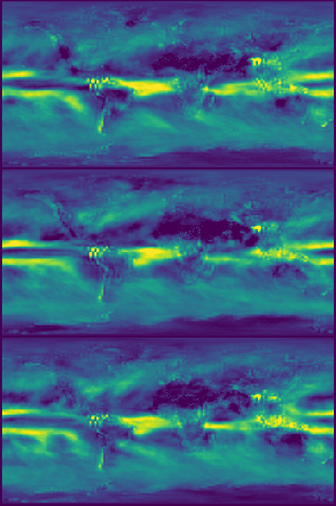
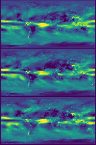
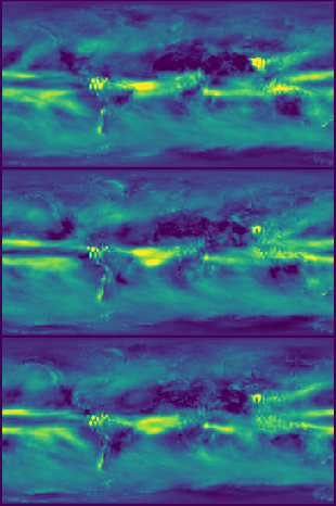
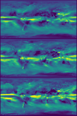
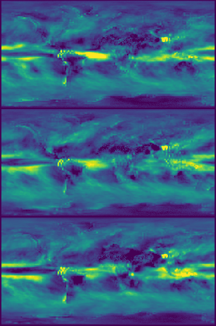
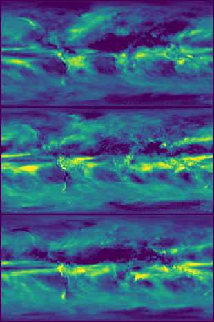
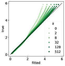
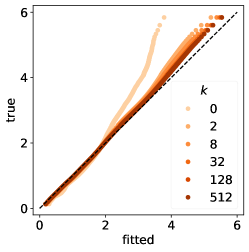
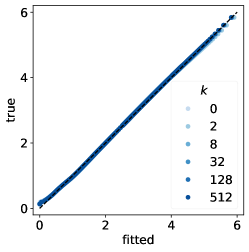
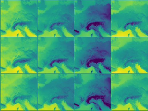
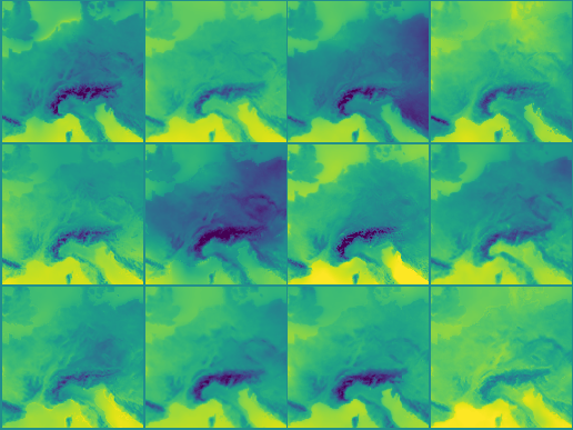
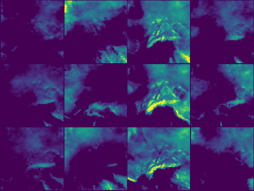
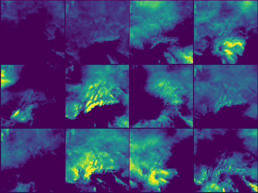
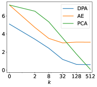
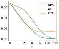
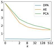
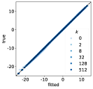
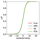
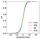
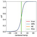
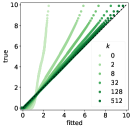
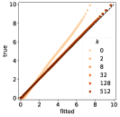
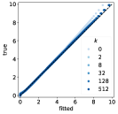
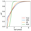
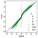
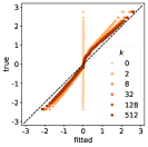
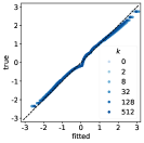
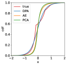
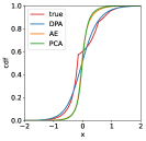
As a motivating example, we consider global monthly precipitation fields on 1 degree latitude-longitude grids for CMIP6 models (Eyring et al.,, 2016; Kravitz et al.,, 2015), resulting in a spatial dimension of . Compressing such high-dimensional spatial fields into a low-dimensional vector loses a large amount of information when aiming for mean reconstructions alone. As shown in Figure 1, reconstructions from PCA or autoencoders tend to smooth out the fields and fail to capture much information about the distribution of precipitation for each location, especially for small latent dimensions. In the extreme case of latent dimension 0, AE just reconstructs any data by the temporal mean precipitation per location. Figure 2 illustrates how quantiles of precipitation at a random location behave for true data versus reconstructions. The high quantiles of the original data are clearly underestimated by AE or PCA reconstructions.
|
True |
|
|
|
|
|
|
|---|---|---|---|---|---|---|
|
PCA |
|
|
|
|
|
|
|
AE |
|
|
|
|
|
|
|
DPA mean |
|
|
|
|
|
|
|
DPA samples |
|
|
|
|
|
|
| PCA | AE | DPA |
|---|---|---|
 |
 |
 |
Here, we develop a nonlinear dimensionality reduction method that first aims at reconstructing data such that the distribution of the reconstructed data is identical to the distribution of the original data. We approach this goal via an encoder-decoder model framework that leverages the expressive capacity of deep neural networks. Denote the data by and assume follows a distribution and denote the latent variables (or, equivalently, embeddings) by with . Similarly to autoencoders, the ‘encoder’, denoted by , is a function from the data space to the latent space. The ‘decoder’ in autoencoders is typically a function that maps samples in the -dimensional latent space back to the original -dimensional space in a way that minimises the mean squared reconstruction error so that ideally
In contrast, our decoder takes as arguments the latent variable and an additional noise variable and maps them to the data space, i.e. . The noise follows a pre-specified distribution such as a standard Gaussian. Instead of focusing merely on mean reconstruction, the aim for our decoder is distributional reconstruction in the following sense. Given an encoder , the decoder tries to achieve
| (1) |
That is, given an embedding , the distribution of the random variable for a random noise input is ideally identical to the conditional distribution of the original data that are mapped by the encoder to the embedding .
If (1) holds true, the distribution of reconstructed data from our decoder is guaranteed to be the same as the original distribution , i.e.
| (2) |
One can view this equality in distribution (2) as a distributional criterion for lossless compression in the sense of retaining the original data distribution. As we will show later, such distributionally lossless compression can be achieved for any compression rate characterised here by the latent dimension .
Our second aim is to learn the ‘principal’ components, analogous to the ones in PCA, while possessing the above distributional properties. Specifically, we want to learn the components in a way that minimises the unexplained variability in a sense made precise in the next section, with the reduction of variance used in PCA being a special case. Moreover, while the latent embeddings in autoencoders are typically disordered, imposing an ordering in the latent space would provide the flexibility to keep only a subset of the latent components, thus enabling an adaptive choice of the latent dimension.
We propose a method Distributional Principal Autoencoder (DPA) that achieves the two goals of distributional reconstruction and minimisation of unexplained variability, simultaneously through a joint formulation of the encoder and decoder. That is,
-
(i)
DPA reconstructions follow the same distribution as the original data, regardless of the number of components retained, and
-
(ii)
DPA embeddings aim to explain the most variability of the data with the flexibility to keep only the first components as the first (nonlinear) principal components for varying .
A more comprehensive description of the method is given in Section 2.
As a concrete example, we illustrate how DPA performs in the global precipitation example earlier. In Figure 1, the last three rows are three reconstructed samples, i.e. samples from the conditional distribution in (1) with for the test data on the top row. Notably, whichever we pick, the reconstructed samples always remain visually realistic as precipitation fields, essentially because they follow the same distribution as the original data, as derived in (2). This is validated further by the Q–Q plots in Figure 2, where DPA captures the full distribution precisely for all choices of , especially the high quantiles, exhibiting a significant advantage over PCA and AE. The visual results also suggest that the variability among different DPA samples decreases as grows larger as more information is retained in the embedding. Furthermore, DPA can also provide mean reconstructions by taking the mean of the reconstructed samples, which leads to similar results as AE, as shown in the fourth row in Figure 1.
In the remainder of the paper, after reviewing the literature, we introduce our methods in Section 2 along with some theoretical justifications. The empirical results presented in Section 3 highlight the effectiveness of DPA in distributional reconstructions and learning meaningful low-dimensional embeddings. In Section 4, we conclude and point out a few outlook of DPA. All proofs are deferred to Appendix A.
1.1 Related work
Our first aim for distributional reconstruction is closely related to the recent literature of generative models whose goal is to learn the data distribution via a transformation of a simple distribution like a Gaussian. However, none of the state-of-the-art deep generative models can directly approach our objectives, including VAE, generative adversarial network (GAN), normalizing flows, and diffusion models. Among them, VAE is the only one that learns an encoder that maps from data to the latent variable. VAE learns the data distribution through variational inference; when using a Gaussian encoder and decoder, the VAE objective becomes a mean squared reconstruction error regularised by the KL divergence between an isotropic Gaussian prior and the variational posterior induced by the encoder:
where denotes the Euclidean norm and is a hyperparameter related to the variance of the Gaussian decoder; see also Higgins et al., (2017). Later AAE (Makhzani et al.,, 2016) and WAE (Tolstikhin et al.,, 2018) extended VAE by replacing the KL term by a distance measure between the aggregated posterior and the prior. All of them have established some theoretical guarantees for (unconditional) generation, yet none for distributional reconstructions in (1) nor (2).
In the original formulation of GAN (Goodfellow et al.,, 2014), only a decoder for (unconditional) generation is learned, while some follow-up work (Dumoulin et al.,, 2017; Donahue et al.,, 2017; Shen et al.,, 2020) extended GAN to an encoder-decoder framework. However, there is no guarantee that these decoders can learn the conditional distribution in (1). Normalizing flows (Papamakarios et al.,, 2021) rely on invertible transformations and diffusion models (Sohl-Dickstein et al.,, 2015; Ho et al.,, 2020) implicitly define the encoder via a stochastic differential equation, both of which require the latent space to be of the same dimension as the data space and are thus unsuitable for dimensionality reduction or distributional reconstruction.
In addition to the distinct target, the specific way we approach distributional reconstruction is also different from the aforementioned generative models. The decoder in the proposed DPA achieves (1) based on proper scoring rules (Gneiting and Raftery,, 2007), which was shown to be effective in the regression setting for learning the conditional distribution of a response variable given a set of predictors (Shen and Meinshausen,, 2023). Here, in contrast, we consider an unsupervised learning setting where only is observed while the latent variables are learned low-dimensional embeddings of .
Related to our second aim for a principal latent space, existing literature has studied extensions of PCA to nonlinear models, resulting in ordered latent representations in neural network architectures. PCA-AE (Pham et al.,, 2022) manually enforces the independence and ordering of a -dimensional latent representation of an autoencoder by learning one latent variable at a time with separate encoders and decoders, thus suffering from a high computational complexity. Nested Dropout (Rippel et al.,, 2014) randomly truncate a hidden layer up to a certain width to encourage ordered representations according to their information content; Triangular Dropout (Staley and Markowitz,, 2022) adopts a similar idea while instead of randomly truncating the hidden layer, its objective function takes an average over the losses for each truncated layer. Ho et al., (2023) presented a unified formulation of both Dropout variants, which under an autoencoder framework looks like
| (3) |
where and denotes the zero vector of dimension . (3) recovers Nested Dropout when ’s forms a geometric distribution and recovers Triangular Dropout when using uniform weights. This formulation shares certain similarities with our procedure adaptive to a varying latent dimension proposed in Section 2.4. However, as autoencoders, their essential goal is still mean reconstruction, whereas our pursuit from a distributional perspective makes our final formulation much more involved than the one above.
1.2 Software
Our method is available in the Python package DistributionalPrincipalAutoencoder with the source code at github.com/xwshen51/DistributionalPrincipalAutoencoder. We plan to release an R version at a later stage.
2 Distributional Principal Autoencoders
We describe our method in this section. We first provide some simple analysis for our encoder and discuss its connections to PCA and AE. In a second step, we propose an approach for learning the decoder that achieves distributional reconstruction. Based on both, we suggest a joint formulation to learn both simultaneously. Finally, we present a procedure that allows an adaptive choice of the latent dimension.
2.1 DPA encoder
The objective of the encoder is to choose an encoding function of data that retains as much information as possible about the original data. To make this notion precise, we first define the so-called oracle reconstructed distribution.
Definition 1 (Oracle reconstructed distribution).
For a given encoder and a sample , the oracle reconstructed distribution, denoted by , is defined as the conditional distribution of , given that its embedding matches the embedding of , i.e.
This distribution reflects how much information about the data is left unexplained knowing its embedding. For example, for a constant encoder , is the same as the original data distribution , as contains no information about ; for an invertible function , is a point mass at .
Then we look for the encoder that maps data to a principal subspace in the sense of minimising the variability in the oracle reconstructed distribution:
| (4) |
where denotes the Euclidean norm and is a hyperparameter.111Here and in the following, the optimisation is with respect to , where is a pre-specified family of possible encoder functions, which can, for example, be a family of linear functions or a neural network class. Without ambiguity, we drop this specification for notational simplicity for both the encoder and, analogously, the decoder. The variability of a distribution is measured in (4) by the expected distance between two independent draws from this distribution. In this way, our encoder ideally collects the maximal possible amount of information about so that the remaining variability is the lowest. As we will see later, when taking , after some reparametrisation, (4) is essentially the same objective as for the encoder in AE or PCA, though we generally adopt .
The following proposition indicates an alternative interpretation of our criterion (4) by showing its equivalence to minimising the reconstruction error, which sheds light on the connections to PCA and AE.
Proposition 1.
For any , we have
The reconstruction error on the right-hand side is measured by the expected distance between a sample of the original data and a sample of the oracle reconstructed distribution .
We will illustrate the connections between our method and PCA through the following example.
Example 1 (Gaussian data and linear encoders).
Assume that follows a multivariate Gaussian distribution with a mean vector and a covariance matrix . Let be the eigendecomposition of , where and with being the eigenvalues. The encoder class is .
The following proposition implies that (4) yields the same subspace as the one spanned by the first principal components from PCA.
Proposition 2.
In general, when taking , the following proposition indicates that (4) yields a solution which together with its corresponding conditional mean leads to the minimum mean squared reconstruction error.
Proposition 3.
When taking , (4) is equal to
This reveals the connection between our formulation and autoencoder which is defined by
| (5) |
Given an encoder , the optimal AE decoder is given by the conditional mean for . Thus, when the decoder is expressive enough, AE obtains the optimal mean reconstruction. However, as demonstrated before, AE does not allow sampling random reconstructions from . In the following, we will describe a procedure to address this.
2.2 DPA decoder
As stated in Section 1, given an encoder, the aim for our decoder is distributional reconstruction (1), which can equivalently be written as for , where is the oracle reconstructed distribution as in Definition 1 and is the embedding value. Note that the oracle reconstructed distribution, by definition, is supported on lower dimensional manifolds (except for ), so is the distribution of . Thus it is unlikely for such two distributions to have a non-empty intersection of their respective support. This makes it difficult to achieve (1) with classical approaches such as maximum likelihood estimation, as the KL divergence is often infinite. We will propose a new approach for this objective.
In addition to distributional reconstruction as its primary objective, a distributional decoder also enables optimisation for the encoder. Proposition 1 indicates the equivalence between the optimisation problem in (4) and choosing an encoder that minimises the following objective, for any ,
| (6) |
We cannot directly minimise this objective function yet, though, as we do not have access to the oracle reconstructed distribution . To this end, we need our decoder to enable sampling from .
We propose to replace the oracle in (6) by the distribution induced by a decoder. Specifically, for any fixed encoder , we define the corresponding decoder by the following optimisation problem:
| (7) |
where denotes the distribution of for any .
The following proposition suggests that when optimised, the minimal value of (7) is the same as the objective function (6).
Proposition 4.
Note that the objective function in (7) with is the expected negative energy score between and the distributional fit . Formally, given an observation and a distribution , the energy score, introduced by Gneiting and Raftery, (2007) as a popular proper scoring rule for evaluating multivariate distributional predictions, is defined as where are two independent draws from and .
2.3 Joint formulation for encoder and decoder
The above results suggest to use (7) as the objective equivalent to the original objectives (6) or (4) for the encoder, which leads to a joint formulation for both the encoder and decoder. Concretely, we define the population version of DPA for a fixed as the solution to the joint optimisation problem that combines (6) and (7) with :
| (8) |
where .
The following proposition justifies how the DPA solution achieves both minimisation of unexplained variability in Section 2.1 and distributional reconstruction in Section 2.2.
Theorem 1.
Consider an encoder class and a decoder class . Assume for any , there exists such that for all . Then the DPA solution defined in (8) satisfies the following.
-
(i)
The DPA encoder minimises the unexplained variability in the sense of (4):
-
(ii)
The DPA decoder induces the oracle reconstructed distribution and hence satisfies for all
After reparametrisation via the decoder, (8) is equivalent to
where and are two independent draws from a standard Gaussian. Note that for a deterministic decoder and , the second term in the objective vanishes and we again recover the AE objective as in (5).
Given an iid sample of data from and an iid sample of noise from , the finite-sample version of DPA is defined via plug-in estimates as
A more detailed algorithm based on the finite-sample loss is given at the end of this section.
2.4 DPA for an adaptive latent dimension
To allow flexibility in selecting the latent dimension, we extend the above DPA procedure for a fixed latent dimension to be valid for multiple , thus allowing an adaptive choice of the retained dimension of the data. Applications for which the reconstruction quality is of high priority would favour a larger , while users with a limited computational or memory budget would typically prefer a smaller , but the choice will also depend on how much information is lost when reducing to smaller latent dimensions. Note that we also include the case of which corresponds to an unconditional generation problem where the decoder, a.k.a. the generator, takes only noise as its input.
We start with describing how the DPA procedure for a fixed proposed in the previous section fits into our current model framework with a varying . For the following, we first expand the latent space to the full dimension of data and later impose constraints to the subspaces in a way that induces an ordering. Specifically, we consider an encoder and a decoder (part of whose arguments can be noise). Let noise which also has the same dimension as data. Consider now any . For the encoder, we simply adopt the criterion in (4) to the first components of our current encoder in , which becomes
while the remaining components of the encoder are left unconstrained for now. For the decoder, the following proposition inspires an adaptive way that allows the decoder to take a varying number of components from the encoder.
Proposition 5.
For any invertible map such that (assume it exists), there exists an optimal decoder such that for all .
It indicates that for any encoder whose distribution coincides with that of (which holds without loss of generality when the encoder is expressive enough), there exists a joint optimal decoder that takes as arguments the first components of encoder and additional -dimensional noise and that matches the oracle reconstructed distribution for all simultaneously.
Motivated by this result, we devise the following procedure to sample from a reconstructed distribution for any :
-
(i)
For a data sample , obtain the latent variable from the encoder, i.e. .
-
(ii)
Keep only the first components of the latent variable while filling the remaining dimensions with i.i.d. standard Gaussian noise entries, i.e. .
-
(iii)
Obtain a reconstructed sample from the decoder, i.e. .
To learn the oracle reconstructed distribution , the decoder formulation in (7) becomes
| (9) |
where denotes the distribution of for any , and . Proposition 5 suggests that defined therein is a solution to (9), simultaneously for all .
Next, to accommodate for multiple ’s simultaneously, we propose to minimise a weighted average of the loss functions for all with respect to a common encoder:
| (10) |
where the weights for all and ; for example, one can take uniform weights . Note that DPA with a fixed introduced in the previous section is a special case of (10) with . In the following proposition, we connect this formulation to PCA.
Proposition 6.
Compared to the result in Proposition 2, with (10), we can recover not only the same subspace as the one obtained by PCA, but also the ordering of the principal directions. Moreover, in this case, the solution to (10) does not depend on the choice of weights as long as all weights are strictly positive, and each term within the summation can be minimised simultaneously. It remains an open problem whether such simultaneous optimality holds more generally. If it cannot hold, the weights will influence the trade-off among different ’s in the optimal solution. We will suggest a default choice of the weights that work well in all our numerical experiments in Section 3. In addition, DPA for a varying latent dimension could also be helpful to guide a choice of the most appropriate latent dimension (which in itself is an open problem for nearly all dimension reduction techniques).
We complete the algorithm for solving (10) via a decoder to match the oracle reconstructed distributions for any given and all , defined as follows:
| (11) |
Based on Proposition 5, we know that there exists a that minimises all the terms for all in the above objective function.
Finally, similar to (8), we define the population version of DPA for varying latent dimensions by a joint formulation that combines (10) and (11):
| (12) |
Similar to Proposition 1, the solution to (12) consists of an optimal encoder and decoder that satisfy (10) and (11), respectively.
In practice, enumerating over is sometimes unnecessary and computationally expensive, especially when is very large. A more efficient and practical way is to consider a subset consisting of all possible numbers of components that one may want to keep.
We parametrize our encoder and decoder by neural networks and solve problem (12) by gradient descent algorithms. We summarize the finite-sample procedure for DPA for varying latent dimensions in Algorithm 1. As noted above, the algorithm includes DPA for a fixed as a special case. For ease of presentation, we present here a gradient descent algorithm with a full-batch of but a mini-batch of of size 2 for each sample. In practice, one can also use a mini-batch of at each gradient step.
3 Empirical results
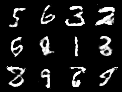
We present empirical studies on data sets across various domains. We first consider two benchmark image data sets: mnist (LeCun and Cortes,, 1998), a data set of hand-written digits, and disk (Ho et al.,, 2023) where each sample is a image consisting of two disks with randomly generated radiuses and x/y-positions for each disk, leading to an intrinsic dimension of 6. We then turn our focus to two scientific scenarios: climate data and single-cell RNA sequencing data. Specifically, we consider monthly regional temperature (r-temp) and precipitation (r-precip) data in central Europe with dimensions of , and global precipitation fields (g-precip) with a dimension of . Additionally, we consider 8 publicly available single-cell data sets (sc1-8) with dimensions ranging from 1k to 6k. See Appendix B for more details of data and all experimental settings.
3.1 Reconstructions
We first investigate the reconstruction performance through visualisations and quantitative metrics. We compare DPA with competitive methods that provide principal/ordered presentations, including PCA and the PCA-variants of AE given in (3) with the same as DPA, which we still call ‘AE’. Throughout all experiments, we use uniform weights .
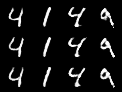
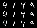
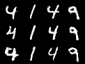
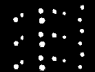
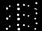
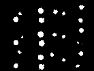
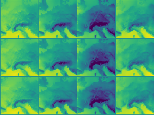
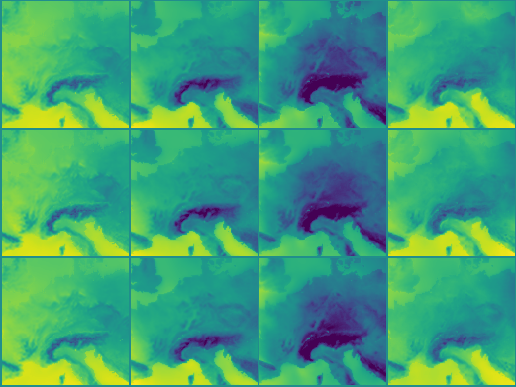
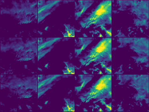
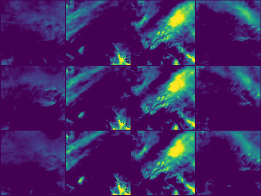
Figures 3-6 demonstrate visually the reconstructions for the 4 image data sets on the held-out test set (results on g-precip were illustrated in Figure 1). For , DPA produces samples from the unconditional data distribution, while PCA and AE degenerate into a point mass at the mean: as shown in the panels on the last column, DPA samples are realistic digits, disks, and regional maps for temperature or precipitation, while PCA and AE reconstructions are just unconditional means of the full data set without much meaningful information. Similar phenomena persist for positive but small ’s, where DPA always generates reasonable samples regardless of whereas PCA and AE tend to blur out the original data. Even for a sufficiently large (as shown in panels on the left), PCA still fails to produce high-quality results due to the lack of nonlinearity, e.g. on mnist and disk, while AE sometimes overfits, leading to unsatisfying reconstruction performance, e.g. in Figure 4. In contrast, DPA reconstructions become fairly close to the raw data as grows, benefited from its expressive model capacity (versus PCA) and not suffering severely from overfitting (versus AE).
|
true |
||||
|---|---|---|---|---|
|
PCA |
||||
|
AE |
||||
|
DPA |
 |
 |
 |
 |
|
true |
|
|
|
|
|
|---|---|---|---|---|---|
|
PCA |
|
|
|
|
|
|
AE |
|
|
|
|
|
|
DPA |
|
|
|
|
|
|
true |
|
|
|
|
|---|---|---|---|---|
|
PCA |
|
|
|
|
|
AE |
|
|
|
|
|
DPA |
|
|
|
|
|
true |
|
|
|
|
|---|---|---|---|---|
|
PCA |
|
|
|
|
|
AE |
|
|
|
|
|
DPA |
|
|
|
|
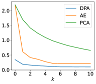
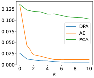
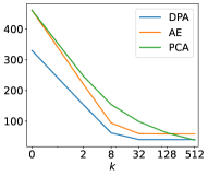
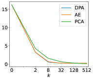
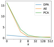
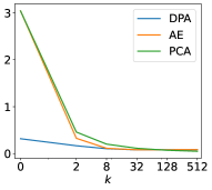
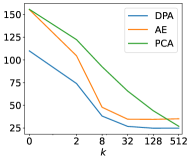
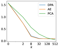
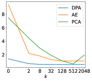
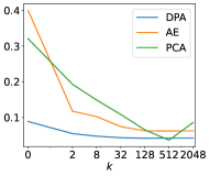
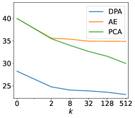
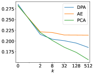
Figure 7 presents several evaluation metrics as functions of the latent dimension . These include
-
(i)
two metrics for conditional reconstruction (1):
-
(a)
conditional energy loss and
-
(b)
mean squared reconstruction error , and
-
(a)
-
(ii)
two metrics for the unconditional distribution of the reconstructions to evaluate how well it matches the original data distribution , i.e. (2):
-
(a)
the energy distance between the two multivariate distributions, i.e. , where and are independent samples, and
-
(b)
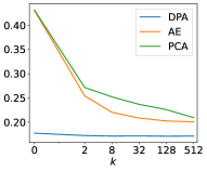
the average Wasserstein 1-distance of the marginal distributions at a random pixel/location, i.e. , where and denote the marginal distributions of the -th component of and , respectively.
-
(a)
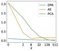
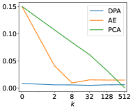
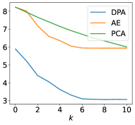
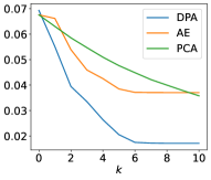
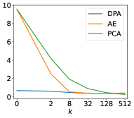
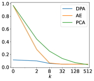
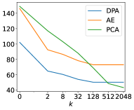
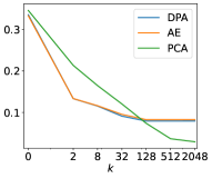
There are three key observations. First, as expected, the conditional metrics are monotonically improving with an increasing latent dimension , which aligns with the visual results that show more variability among the DPA samples (conditional on same input) when using a smaller dimension . Interestingly, the conditional metrics typically reach a plateau after increasing the latent dimension above a certain value, which would correspond roughly to the intrinsic dimension of data. For example, the conditional metrics for disk decreases until which matches exactly the intrinsic dimension of this data set (due to the 6 generative factors). Second, recall that AE and PCA use the mean squared reconstruction error as their loss function whereas DPA aims for the full distribution. Thus ideally, when the model class is expressive enough, AE and DPA should have the same and minimal conditional MSEs while PCA may suffer a bit due to the limitation of linear models. As shown in the second column, this is indeed the case for the three climate data sets with large enough samples sizes. However, for the remaining three data sets whose samples sizes are not as large, DPA exhibits smaller MSEs than AE, especially on disk, which is potentially because DPA suffers less from overfitting than AE does. These findings indicate the DPA performs at least as well as AE in terms of mean reconstruction (the objective of AE), even though its objective is distributional reconstruction. Third, DPA outperforms AE and PCA significantly in terms of the unconditional metrics, as only DPA is guaranteed to produce reconstructions that are identically distributed as the original data. Moreover, such guarantee holds for all , and it indeed turns out that the unconditional metrics stay almost constant for all .
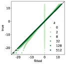
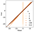
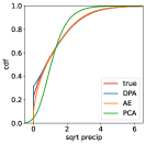
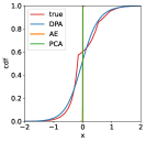
To further investigate how well our reconstructed distributions match the original ones, in Figure 8, we show Q–Q plots and empirical cdfs of the true or estimated marginal distributions at a random location. We observe that DPA captures the distribution the best regardless of the choice of . This is especially true for the tail behaviour. In contrast, the tails of the distribution get shifted towards the mean with PCA and AE, especially for smaller ’s and as expected due to their reconstructions trying to minimise the mean squared error.
| conditional energy loss | conditional MSE | uncond energy distance | marginal W distance | |
|---|---|---|---|---|
|
mnist |
 |
 |
 |
 |
|
disk |
 |
 |
 |
 |
|
r-temp |
 |
 |
 |
 |
|
r-precip |
 |
 |
 |
 |
|
g-precip |
 |
 |
 |
 |
|
sc-8 |
 |
 |
 |
 |
| Q–Q plots | empirical cdfs | |||||
|
r-temp |
 |
 |
 |
 |
 |
 |
|
r-precip |
 |
 |
 |
 |
 |
 |
|
sc-8 |
 |
 |
 |
 |
 |
 |
| PCA | AE | DPA | ||||
3.2 Embeddings
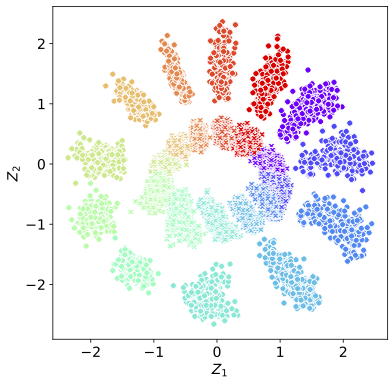
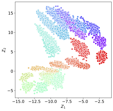
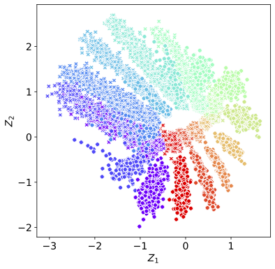
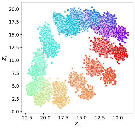
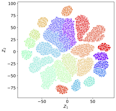
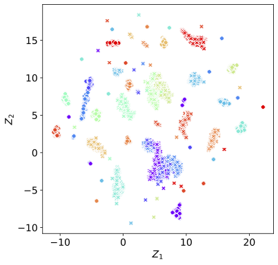
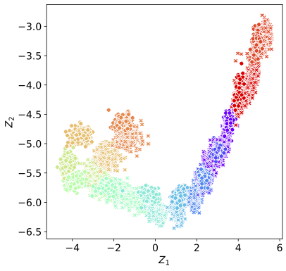
In many scientific applications, it is useful to visualise high-dimensional data in a 2-dimensional latent space. Here, we investigate how well the 2D principal components obtained by DPA can preserve the underlying structure in data. We consider global precipitation data and 8 single-cell data sets. For competitive methods, we adopt PCA, AE, VAE, WAE, as well as the state-of-the-art methods for data visualisation, t-SNE (Van der Maaten and Hinton,, 2008) and UMAP (McInnes et al.,, 2018).
In Figure 9, we visualise the 2D embeddings for global precipitation fields obtained by different methods. The training data consists of 12 months and are simulated by different general circulation models each corresponding to a slightly different physical mechanism and thus a distinct distribution. In the top-left panel, DPA embeddings preserve such underlying structures very well: (i) the seasonal cycle is precisely captured through the angle and (ii) data from different models are well separated according to the radius in the latent space. The embeddings obtained by all other methods share at most one of these two appealing features. Specifically, PCA and WAE embeddings are able to reflect some seasonal cycle, though they tend to mix up winter months and neither can they fully separate data from different models. With t-SNE, different models and months are well separated, but there is no structural pattern preserved in its 2D latent space. UMAP overly disperses the patterns while AE and VAE embeddings also do not provide much meaningful information.
In Table 1, we report for the single cell data sets the k-nearest neighbour accuracy of classifying the cell type based on the 2D embeddings. We use five neighbours throughout. For all eight data sets, DPA always stands out with the highest or second highest accuracy, suggesting that the 2D DPA embeddings preserve the local structure of high-dimensional gene expressions well. Among previous methods, AE and WAE are the most competitive ones, though often inferior to DPA. Note that t-SNE and UMAP do not produce an explicit mapping to the low-dimensional latent space and can hence not be evaluated on new test data. For evaluation, we need to run them on test data and hence exclude them in the ranking in Table 1. Despite this, the k-NN accuracy of DPA is often not too far those of t-SNE and UMAP, and sometimes even better, e.g. on sc1, sc6, and sc7.
| DPA | AE | WAE | |
|---|---|---|---|
 |
 |
 |
| PCA | t-SNE | UMAP | VAE |
|---|---|---|---|
 |
 |
 |
 |
| sc1 | sc2 | sc3 | sc4 | sc5 | sc6 | sc7 | sc8 | |
| DPA | 0.659 | 0.882 | 0.285 | 0.830 | 0.858 | 0.802 | 0.792 | 0.521 |
| AE | 0.643 | 0.877 | 0.219 | 0.793 | 0.850 | 0.764 | 0.790 | 0.513 |
| VAE | 0.570 | 0.868 | 0.137 | 0.730 | 0.714 | 0.734 | 0.752 | 0.501 |
| WAE | 0.623 | 0.849 | 0.246 | 0.787 | 0.819 | 0.722 | 0.804 | 0.535 |
| PCA | 0.483 | 0.839 | 0.170 | 0.670 | 0.540 | 0.513 | 0.300 | 0.440 |
| t-SNE | 0.554 | 0.901 | 0.537 | 0.970 | 0.920 | 0.757 | 0.662 | 0.594 |
| UMAP | 0.393 | 0.890 | 0.430 | 0.960 | 0.892 | 0.757 | 0.562 | 0.559 |
4 Discussion
We proposed DPA as a dimension reduction technique with the following properties:
-
(i)
As in Principal Component Analysis (PCA), the latent space is ordered according to how much variability of data being explained so that users are free to keep a few latent components (with high compression of the data but larger variability unexplained) or a large number of latent variables (with lower compression but less remaining variability).
-
(ii)
As in autoencoders (AE), mappings for dimension reduction and data reconstruction are nonlinear with deep neural networks.
-
(iii)
Unlike PCA, AE, or variants like VAE and WAE, our decoder aims to produce samples from the oracle reconstructed distribution, namely the conditional distribution of the original data that leads to the given embedding value, using an energy-score based loss function.
The last property ensures that the reconstructed data follow in population the same distribution as the original data, hence yielding ‘distributionally lossless’ compression, irrespective of the dimension of the latent variable that is being used.
There are several facets of DPA that are worth exploring further. Here we outline a few directions that we find particularly intriguing.
Arguably one of the biggest characteristics of DPA is its ability to reconstruct the full distribution from the latent embeddings: encoding the data into a low-dimensional latent space and then decoding again will not change the distribution in population for DPA. In contrast, doing the same for PCA and AE and variants will alter the data distribution drastically, especially in the tails of the distribution since their decoder is aiming for a conditional mean prediction, not aiming to estimate the full oracle reconstructed distribution. Due to the ability of DPA to provide distributional reconstruction and hence maintain the original data distribution, we envisage applications for characterising distribution shifts, transport between high-dimensional distributions, and prediction problems with very high-dimensional responses.
One example is transport between high-dimensional distributions through the DPA latent space. For instance, the data is a mixture of two high-dimensional distributions and and the goal is to transport from to , for which the optimal transport in the high-dimensional space is often intractable. Now with DPA, the latent variables also follow a mixture of distributions; denote when , for . The optimal transport from to in the low-dimensional (e.g. 2D) latent space becomes much more tractable. More importantly, the distributional reconstruction ability of DPA guarantees that after transportation from to in the latent space and decoding back to the original space, the decoded distribution of transported latents will match the target high-dimensional distribution . In the context of the climate data examples mentioned, this opens up the possibility of correcting the bias of climate models () with respect to the observational data () by transportation from model data to match the full distribution of the observational data, rather than just to match the first one or two moments as in conventional bias correction techniques. And the visualisations of DPA embeddings in Figure 9 suggest that a transport from model 0 to model 1 in the 2D latent space could be as simple as increasing the radius by a factor of 2 roughly.
In addition, the latent subspace identified by DPA is generally different from that by existing methods like PCA and AE. The numerical results for climate and single cell data in Section 3.2 show how DPA improves the embeddings of PCA and AE in some metrics. For example, the DPA embeddings exhibit better separation between different temporal patterns or cell types. As another example, consider bivariate isotropic data where one component follows a uniform distribution and the other one follows a t-distribution. PCA, in this case, would pick an arbitrary direction as its first principal subspace, whereas DPA with a linear encoder would favour the light-tailed component over the heavy-tailed one. Such distinction leads to potential new identification results of the latent variables, which is relevant to the emerging field of causal representation learning (Khemakhem et al.,, 2020; Kivva et al.,, 2022).
References
- Bengio et al., (2013) Bengio, Y., Yao, L., Alain, G., and Vincent, P. (2013). Generalized denoising auto-encoders as generative models. Advances in neural information processing systems, 26.
- Candès et al., (2011) Candès, E. J., Li, X., Ma, Y., and Wright, J. (2011). Robust principal component analysis? Journal of the ACM (JACM), 58(3):1–37.
- Copernicus Climate Change Service, (2019) Copernicus Climate Change Service, C. D. S. (2019). Cordex regional climate model data on single levels. copernicus climate change service (c3s) climate data store (cds).
- Donahue et al., (2017) Donahue, J., Krähenbühl, P., and Darrell, T. (2017). Adversarial feature learning. In ICLR.
- Dumoulin et al., (2017) Dumoulin, V., Belghazi, I., Poole, B., Lamb, A., Arjovsky, M., Mastropietro, O., and Courville, A. C. (2017). Adversarially learned inference. In ICLR.
- Eyring et al., (2016) Eyring, V., Bony, S., Meehl, G. A., Senior, C. A., Stevens, B., Stouffer, R. J., and Taylor, K. E. (2016). Overview of the coupled model intercomparison project phase 6 (cmip6) experimental design and organization. Geoscientific Model Development, 9(5):1937–1958.
- Gneiting and Raftery, (2007) Gneiting, T. and Raftery, A. E. (2007). Strictly proper scoring rules, prediction, and estimation. Journal of the American statistical Association, 102(477):359–378.
- Goodfellow et al., (2014) Goodfellow, I., Pouget-Abadie, J., Mirza, M., Xu, B., Warde-Farley, D., Ozair, S., Courville, A., and Bengio, Y. (2014). Generative adversarial nets. Advances in neural information processing systems, 27.
- Hao et al., (2023) Hao, Y., Stuart, T., Kowalski, M. H., Choudhary, S., Hoffman, P., Hartman, A., Srivastava, A., Molla, G., Madad, S., Fernandez-Granda, C., and Satija, R. (2023). Dictionary learning for integrative, multimodal and scalable single-cell analysis. Nature Biotechnology.
- Higgins et al., (2017) Higgins, I., Matthey, L., Pal, A., Burgess, C. P., Glorot, X., Botvinick, M. M., Mohamed, S., and Lerchner, A. (2017). beta-vae: Learning basic visual concepts with a constrained variational framework. In International Conference on Learning Representations.
- Hinton and Salakhutdinov, (2006) Hinton, G. E. and Salakhutdinov, R. R. (2006). Reducing the dimensionality of data with neural networks. science, 313(5786):504–507.
- Ho et al., (2020) Ho, J., Jain, A., and Abbeel, P. (2020). Denoising diffusion probabilistic models. Advances in neural information processing systems, 33:6840–6851.
- Ho et al., (2023) Ho, M., Zhao, X., and Wandelt, B. (2023). Information-ordered bottlenecks for adaptive semantic compression. arXiv preprint arXiv:2305.11213.
- Jolliffe, (2002) Jolliffe, I. (2002). Principal Component Analysis. Springer Series in Statistics. Springer.
- Khemakhem et al., (2020) Khemakhem, I., Kingma, D., Monti, R., and Hyvarinen, A. (2020). Variational autoencoders and nonlinear ica: A unifying framework. In International Conference on Artificial Intelligence and Statistics, pages 2207–2217. PMLR.
- Kingma and Ba, (2015) Kingma, D. P. and Ba, J. (2015). Adam: A method for stochastic optimization. In Proceedings of the 3rd International Conference on Learning Representations (ICLR).
- Kingma and Welling, (2014) Kingma, D. P. and Welling, M. (2014). Auto-encoding variational bayes. In International Conference on Learning Representations.
- Kivva et al., (2022) Kivva, B., Rajendran, G., Ravikumar, P., and Aragam, B. (2022). Identifiability of deep generative models without auxiliary information. Advances in Neural Information Processing Systems, 35:15687–15701.
- Kravitz et al., (2015) Kravitz, B., Robock, A., Tilmes, S., Boucher, O., English, J. M., Irvine, P. J., Jones, A., Lawrence, M. G., MacCracken, M., Muri, H., Moore, J. C., Niemeier, U., Phipps, S. J., Sillmann, J., Storelvmo, T., Wang, H., and Watanabe, S. (2015). The geoengineering model intercomparison project phase 6 (geomip6): simulation design and preliminary results. Geoscientific Model Development, 8(10):3379–3392.
- LeCun and Cortes, (1998) LeCun, Y. and Cortes, C. (1998). The mnist database of handwritten digits. http://yann.lecun.com/exdb/mnist/.
- Majumdar and Majumdar, (2019) Majumdar, R. and Majumdar, S. (2019). On the conditional distribution of a multivariate normal given a transformation–the linear case. Heliyon, 5(2).
- Makhzani et al., (2016) Makhzani, A., Shlens, J., Jaitly, N., Goodfellow, I., and Frey, B. (2016). Adversarial autoencoders. In International Conference on Learning Representations.
- McInnes et al., (2018) McInnes, L., Healy, J., Saul, N., and Großberger, L. (2018). Umap: Uniform manifold approximation and projection. Journal of Open Source Software, 3(29):861.
- Papamakarios et al., (2021) Papamakarios, G., Nalisnick, E., Rezende, D. J., Mohamed, S., and Lakshminarayanan, B. (2021). Normalizing flows for probabilistic modeling and inference. Journal of Machine Learning Research, 22(57):1–64.
- Pham et al., (2022) Pham, C.-H., Ladjal, S., and Newson, A. (2022). Pca-ae: Principal component analysis autoencoder for organising the latent space of generative networks. Journal of Mathematical Imaging and Vision, 64(5):569–585.
- Rippel et al., (2014) Rippel, O., Gelbart, M., and Adams, R. (2014). Learning ordered representations with nested dropout. In International Conference on Machine Learning, pages 1746–1754. PMLR.
- Rumelhart et al., (1986) Rumelhart, D. E., Hinton, G. E., and Williams, R. J. (1986). Learning representations by back-propagating errors. nature, 323(6088):533–536.
- Shen and Meinshausen, (2023) Shen, X. and Meinshausen, N. (2023). Engression: Extrapolation for nonlinear regression? arXiv preprint arXiv:2307.00835.
- Shen et al., (2020) Shen, X., Zhang, T., and Chen, K. (2020). Bidirectional generative modeling using adversarial gradient estimation. arXiv preprint arXiv:2002.09161.
- Sohl-Dickstein et al., (2015) Sohl-Dickstein, J., Weiss, E., Maheswaranathan, N., and Ganguli, S. (2015). Deep unsupervised learning using nonequilibrium thermodynamics. In International conference on machine learning, pages 2256–2265. PMLR.
- Staley and Markowitz, (2022) Staley, E. W. and Markowitz, J. (2022). Triangular dropout: Variable network width without retraining. arXiv preprint arXiv:2205.01235.
- Székely, (2003) Székely, G. J. (2003). E-statistics: The energy of statistical samples. Bowling Green State University, Department of Mathematics and Statistics Technical Report, 3(05):1–18.
- Székely and Rizzo, (2023) Székely, G. J. and Rizzo, M. L. (2023). The Energy of Data and Distance Correlation. CRC Press.
- Tolstikhin et al., (2018) Tolstikhin, I., Bousquet, O., Gelly, S., and Schoelkopf, B. (2018). Wasserstein auto-encoders. In International Conference on Learning Representations.
- Van der Maaten and Hinton, (2008) Van der Maaten, L. and Hinton, G. (2008). Visualizing data using t-sne. Journal of machine learning research, 9(11).
- Yu et al., (2011) Yu, S., Tranchevent, L.-C., De Moor, B., and Moreau, Y. (2011). Kernel-based data fusion for machine learning. Studies in Computational Intelligence: Springer Berlin Heidelberg.
Appendix A Proofs
Proof of Proposition 1.
Let with a joint density and denote by the conditional density of given . Write the density of as Then we have
where comes from the fact that any samples from satisfy almost surely for all ; thus only when . ∎
Proof of Proposition 2.
According to Majumdar and Majumdar, (2019, Theorem 4), the conditional distribution of given , denoted by , is , where
Then by Proposition 1, the objective function in (4) becomes
where and are two independent draws from . Now formulation (4) is equivalent to
According to Yu et al., (2011, Theorem 2.3), the solution to the above problem is given by up to column permutations. Then we conclude the desired result. ∎
Proof of Proposition 3.
The following lemma based on the results in Székely, (2003) and Székely and Rizzo, (2023) states that the energy score is a strictly proper scoring rule.
Lemma 1.
For any distribution , we have
where the equality holds if and only if and are identical.
Proof of Proposition 4.
When and , the objective function in (7) is equal to
| (13) |
Given , it is the expected energy score between the oracle reconstructed distribution and the reconstructed distribution induced by the decoder :
By Lemma 1, we know that the above objective is minimised if and only if and are identical with the minimal value
for all . The assumption guarantees the existence of such optimal decoders that for any . Thus also minimises (13) with the minimal value (7) given by
where the equality is due to Proposition 1 and the right-hand side is exactly (6) with . ∎
Proof of Theorem 1.
Proof of Proposition 5.
Let be such that for all . As with independent components, we have for all . This implies that the conditional distribution of given is equal to the conditional distribution of given . ∎
Appendix B Experimental details
B.1 Data sets and preprocessing
Benchmark image data:
-
•
mnist: 6k training samples. Each sample is a image of hand-written digits (from 0 to 9) with pixel values in .
-
•
disk: 10k training samples. Each sample is a image of two disks with pixel values in . Each disk is determined by three generative factors: x-position, y-position, and radius, all of which are randomly sampled. In total the intrinsic dimension is 6.
Climate data:
-
•
r-temp: regional temperature data from CORDEX models (Copernicus Climate Change Service,, 2019) in Kelvin. The sample size is 167,645. We center the data by the temporal mean per location.
-
•
r-precip: regional precipitation data from CORDEX models (Copernicus Climate Change Service,, 2019) model. The unit of the raw precipitation data is . Sample size is 167,645.
- •
Single-cell data: we consider 8 data sets from the R package SeuratData and follow the standard preprocessing procedures provided in the R toolkit Seurat (Hao et al.,, 2023) for single-cell genomics, including log transformation and standardization. We pre-select the genes with more than 20% expressed cells (with nonzero counts). Table 2 lists the details for each data set.
| name | data set | dimension | sample size |
|---|---|---|---|
| sc1 | bmcite | 918 | 30672 |
| sc2 | cbmc | 1118 | 7895 |
| sc3 | celegans_embryo | 1019 | 4883 |
| sc4 | mousecortex | 3005 | 558 |
| sc5 | panc8 | 6810 | 14890 |
| sc6 | pbmc3k | 943 | 2638 |
| sc7 | pbmcsca | 810 | 31021 |
| sc8 | thp1_eccite | 5806 | 20729 |
B.2 Hyperparameters
For the energy score used in DPA, we always use the default choice of . Throughout all experiments, we keep the hyperparameters for neural network architectures and optimisation the same for all deep learning based methods including AE, VAE, and WAE. Specifically, we use the Adam optimiser (Kingma and Ba,, 2015) with a learning rate of , default values for the beta parameters, and a mini-batch size of 512.
For the neural network architecture, we always adopt multilayer perceptrons (MLPs) (we vectorize image/spatial data). The encoder is a standard MLP while the decoder has to take random noises as arguments, so we adopt the architecture used by Shen and Meinshausen, (2023). As some of our neural nets are fairly deep, we use skip-connections every two-layer. Experiments for DPA and AE for varying ’s in Section 3.1 require rich enough model classes, so we use encoders and decoders with 16 layers; the numbers of neurons per layer are 512 for mnist and disk, 1000 for all single-cell data sets, 5000 for r-temp and r-precip, and 2048 for g-precip, which are rather arbitrary choices mainly to fit into the GPU memory. For the decoder, we concatenate to each layer a 100-dimensional standard Gaussian noise except for the global precipitation data with the highest dimension and complexity for which we concatenate a 500-dimensional Gaussian noise. Experiments in Section 3.2 are only for a latent dimension of 2, so we use shallower networks with 4 layers for both encoders and decoders, and we keep the same network width as before. All experiments are run on a single NVIDIA RTX 4090 GPU.
For non-deep learning methods, we use the Python scikit-learn library for PCA, UMAP, and t-SNE with the default parameters. For g-precip with a very high dimension and sample size so that the data could not be loaded into the memory, we train a linear autoencoder with mean squared reconstruction error (with intercepts) and Adam optimiser with the same hyperparameter settings.