Mean Aggregator Is More Robust Than Robust Aggregators
Under Label Poisoning Attacks

Abstract

Robustness to malicious attacks is of paramount importance for distributed learning. Existing works often consider the classical Byzantine attacks model, which assumes that some workers can send arbitrarily malicious messages to the server and disturb the aggregation steps of the distributed learning process. To defend against such worst-case Byzantine attacks, various robust aggregators have been proven effective and much superior to the often-used mean aggregator. In this paper, we show that robust aggregators are too conservative for a class of weak but practical malicious attacks, as known as label poisoning attacks, where the sample labels of some workers are poisoned. Surprisingly, we are able to show that the mean aggregator is more robust than the state-of-the-art robust aggregators in theory, given that the distributed data are sufficiently heterogeneous. In fact, the learning error of the mean aggregator is proven to be optimal in order. Experimental results corroborate our theoretical findings, demonstrating the superiority of the mean aggregator under label poisoning attacks.

1 Introduction

With the rising and rapid development of large machine learning models, distributed learning attracts more and more attention by researchers due to its provable effectiveness in solving large-scale problems Verbraeken et al. (2020). In distributed learning, there often exist one parameter server (called server thereafter) owing the global model and some computation devices (called workers thereafter) owing the local data. In the training process, the server sends the global model to the workers, and the workers use their local data to compute the local gradients on the global model and send them back to the server. Upon receiving the local gradients from all workers, the server aggregates them and uses the aggregated gradient to update the global model. After the training process, the trained global model is evaluated on the testing data. One important application of distributed learning is federated learning Ye et al. (2023); Gosselin et al. (2022); Yang et al. (2019); McMahan et al. (2017), which is particularly favorable in terms of privacy preservation.

However, the distributed nature of the server-worker architecture is vulnerable to malicious attacks during the learning process. Due to data corruptions, equipment failures, or cyber attacks, some workers may not follow the algorithmic protocol and send incorrect messages to the server. Previous works often characterize these attacks by the classical Byzantine attacks model, which assumes that some workers can send arbitrarily malicious messages to the server so that the aggregation steps of the learning process is disturbed Lamport et al. (1982). For such worst-case Byzantine attacks, various robust aggregators have been proven effective and much superior to the mean aggregator Chen et al. (2017); Xia et al. (2019); Karimireddy et al. (2021); Wu et al. (2023).

The malicious attacks encountered in reality, on the other hand, are often less destructive than the worst-case Byzantine attacks. For example, a distributed learning system may often suffer from label poisoning attacks, which are weak yet of practical interest. Considering a highly secure email system in a large organization (for example, government or university), if hackers (some users) aim to disturb the online training process of a spam detection model, one of the most effective ways for them is to mislabel received emails from “spam” to “non-spam”, resulting in label poisoning attacks. Similar attacks may happen in fraudulent short message service (SMS) detection held by large communication corporations, too.

To this end, in this paper, we consider label poisoning attacks where some workers have local data with poisoned labels and compute the incorrect messages during the learning process. Under label poisoning attacks and with some mild assumptions, surprisingly we are able to show that the mean aggregator is more robust than the state-of-the-art robust aggregators in theory, given that the distributed data are sufficiently heterogeneous. The main contributions of this paper are summarized as follows.

C1) To the best of our knowledge, our work is the first to investigate the robustness of the mean aggregator under attacks in distributed learning. Our work reveals an important fact that the mean aggregator is more robust than the existing robust aggregators under specific types of malicious attacks, which motivates us to rethink the usage of different aggregators within practical scenarios.

C2) Under label poisoning attacks, we theoretically analyze the learning errors of the mean aggregator and the state-of-the-art robust aggregators. The results show that when the heterogeneity of the distributed data is large, the learning error of the mean aggregator is optimal in order regardless of the fraction of poisoned workers.

C3) We empirically evaluate the performance of the mean aggregator and the existing robust aggregators under label poisoning attacks. The experimental results fully support our theoretical findings.

2 Related Works

Poisoning attacks can be categorized into targeted attacks and untargeted attacks; or model poisoning attacks and data poisoning attacks Kairouz et al. (2021). In this paper, we focus on the latter categorization. In model poisoning attacks, the malicious workers transmit arbitrarily poisoned models to the server, while data poisoning attacks yield poisoned messages by fabricating poisoned data at the malicious workers’ side Shejwalkar et al. (2022). Below we briefly review the related works of the two types of poisoning attacks in distributed learning, respectively.

Under model poisoning attacks, most of the existing works design robust aggregators for aggregating local gradients of workers and filter out the potentially poisoned messages. The existing robust aggregators include Krum Blanchard et al. (2017), geometric median Chen et al. (2017), coordinate-wise median Yin et al. (2018), coordinate-wise trimmed-mean Yin et al. (2018), FABA Xia et al. (2019), centered clipping Karimireddy et al. (2021), etc. The key idea behind these robust aggregators is to find a point that has bounded distance to the true gradient such that the learning error is under control. Farhadkhani et al. (2022a) and Allouah et al. (2023) propose a unified framework to analyze the performance of these robust aggregators under attacks. Though these methods work well when the data distributions are the same over the workers, their performance degrades when the data distributions become heterogeneous Karimireddy et al. (2022); Li et al. (2019). To address this issue, Li et al. (2019) suggests using model aggregation rather than gradient aggregation to defend against model poisoning attacks in the heterogeneous case. Karimireddy et al. (2022); Peng et al. (2022); Allouah et al. (2023) propose to use the bucketing/resampling and nearest neighbor mixing techniques to reduce the heterogeneity of the gradients, prior to aggregation. There also exist some works focusing on decentralized optimization without a server, under model poisoning attacks Wu et al. (2023); He et al. (2022); Peng et al. (2021). Nevertheless, we focus on distributed learning with a server in this paper.

There are a large amount of papers focusing on data poisoning attacks Bagdasaryan et al. (2020); Wang et al. (2020); Sun et al. (2019); Rosenfeld et al. (2020). To defend against data poisoning attacks, the existing works use data sanitization to remove poisoned data Steinhardt et al. (2017), and prune activation units that are inactive on clean data Liu et al. (2018). For more defenses against data poisoning attacks, we refer the reader to the survey paper Kairouz et al. (2021).

In practice, however, attacks may not necessarily behave as arbitrarily malicious as the above well-established works consider. Some weaker attacks models are structured; for example, Tavallali et al. (2022) considers the label poisoning attacks in which some workers mislabel their local data and compute the incorrect messages using those poisoned data. Specifically, Tolpegin et al. (2020); Lin et al. (2021); Jebreel et al. (2024); Jebreel and Domingo-Ferrer (2023) consider the case where some workers flip the labels of their local data from source classes to target classes. Notably, label poisoning is a kind of data poisoning but not necessarily the worst-case attack, since label poisoning attacks fabricates the local data, yet only on the label level.

It has been shown that label poisoning attacks are equivalent to model poisoning attacks in essence Farhadkhani et al. (2022b). Therefore, defenses designed for model poisoning attacks are still effective, including Krum, geometric median, coordinate-wise median, coordinate-wise trimmed-mean, FABA, and centered clipping, as validated by Karimireddy et al. (2022); Gorbunov et al. (2022); Fang et al. (2020). There also exist some works designing robust aggregators based on specific properties of label poisoning. For example, the work of Tavallali et al. (2022) proposes regularization-based defense to detect and exclude the samples with flipped labels in the training process. However, Tavallali et al. (2022) requires to access a clean validation set, which has privacy concerns in distributed learning. Another work named as LFighter Jebreel et al. (2024), is the state-of-the-art defense for label poisoning attacks in federated learning. Jebreel et al. (2024) proposes to cluster the local gradients of all workers, identify the smaller and denser clusters as the potentially poisoned gradients, and discard them. The key idea of LFighter is that the difference between the gradients connected to the source and target output neurons of poisoned workers and regular workers becomes larger when the training process evolves. Therefore it is able to identify the potentially poisoned gradients. However, LFighter only works well when data distributions at different workers are similar. If the heterogeneity of the distributed data is large, the performance of LFighter degrades, as we will show in Section 5.

A recent work of Shejwalkar et al. (2022), similar to our findings, reveals the robustness of the mean aggregator under poisoning attacks in production federated learning systems. Nevertheless, their study is restrictive in terms of the poisoning ratio (for example, less than 0.1% workers are poisoned while we can afford 10% in the numerical experiments) and lacks theoretical analysis. In contrast, we provide both theoretical analysis and experimental validations.

In conclusion, our work is the first one to investigate the robustness of the mean aggregator under attacks in distributed learning. It reveals an important fact that robust aggregators cannot always outperform the mean aggregator under specific attacks, promoting us to rethink the application scenarios for the use of robust aggregators.

3 Problem Formulation

Consider a distributed learning system with one server and $W$ workers. Denote the set of workers as $\mathcal{W}$ with $|\mathcal{W}|=W$, and the set of regular workers as $\mathcal{R}$ with $|\mathcal{R}|=R$. Note that the number and identities of the regular workers are unknown. Our goal is to solve the following distributed learning problem defined over the regular workers in $\mathcal{R}$, at the presence of the set of poisoned workers $\mathcal{W}\setminus\mathcal{R}$:

$$\min_{x\in{\mathbb{R}}^{D}}f(x) \triangleq\frac{1}{R}\sum_{w\in\mathcal{R}}f_{w}(x),$$ (1)

$$\text{with }\ f_{w}(x) \triangleq\frac{1}{J}\sum_{j=1}^{J}f_{w,j}(x),\ \ \forall w\in\mathcal{R}.$$

Here, $x\in{\mathbb{R}}^{D}$ is the global model, and $f_{w}(x)$ is the local cost of worker $w\in\mathcal{R}$ that averages the costs $f_{w,j}(x)$ of $J$ samples. Without loss of generality, we assume that all workers have the same number of samples $J$.

We begin with characterizing the behaviors of the poisoned workers in $\mathcal{W}\setminus\mathcal{R}$. Different to the classical Byzantine attacks model that assumes some workers to disobey the algorithmic protocol and send arbitrarily malicious messages to the server Lamport et al. (1982), here we assume the poisoned workers to: (i) have samples with poisoned labels; (ii) exactly follow the algorithmic protocol during the distributed learning process. The formal definition is given as follows.

Definition 1 (Label poisoning attacks).

In solving (1), there exist a number of poisoned workers, whose local costs are in the same form as the regular workers but a fraction of sample labels are poisoned. Nevertheless, these poisoned workers exactly follow the algorithmic protocol during the distributed learning process.

To solve (1) with the distributed gradient descent algorithm, the server needs to average the local gradients of the regular workers at each iteration. However, as we have emphasized, the number and identities of the regular workers are unknown, such that the server cannot distinguish the true local gradients of the regular workers and the poisoned local gradients from the poisoned workers. We call the true and poisoned local gradients as messages, which the server must judiciously aggregate.

Let the global model be $x^{t}$ at iteration $t$. Denote the true local gradient of regular worker $w\in\mathcal{R}$ as $\nabla f_{w}(x^{t})$ and the poisoned local gradient of poisoned worker $w\in\mathcal{W}\setminus\mathcal{R}$ as $\nabla\tilde{f}_{w}(x^{t})$. For notational convenience, we denote the message sent by worker $w$, no matter true or poisoned, as:

$$\nabla\hat{f}_{w}(x^{t})=\left\{\begin{aligned} &\nabla f_{w}(x^{t}),&&w\in\mathcal{R},\\ &\nabla\tilde{f}_{w}(x^{t}),&&w\in\mathcal{W}\setminus\mathcal{R}.\end{aligned}\right.$$ (2)

Upon receiving all the messages $\{\nabla\hat{f}_{w}(x^{t}):w\in\mathcal{W}\}$, the server can aggregate them with a robust aggregator $\text{RAgg}(\cdot)$ and then move a step along the negative direction:

$$x^{t+1}=x^{t}-\gamma\cdot\text{RAgg}(\{\nabla\hat{f}_{w}(x^{t}):w\in\mathcal{W}\}),$$ (3)

where $\gamma>0$ is the step size. State-of-the-art robust aggregators include trimmed mean (TriMean) Chen et al. (2017), centered clipping (CC) Karimireddy et al. (2021), FABA Xia et al. (2019), to name a few.

In this paper, we argue that the mean aggregator $\text{Mean}(\cdot)$, which is often viewed as vulnerable, is more robust than state-of-the-art robust aggregators under label poisoning attacks. With the mean aggregator, the update is

$$x^{t+1}=x^{t}-\gamma\cdot\text{Mean}(\{\nabla\hat{f}_{w}(x^{t}):w\in\mathcal{W}\}),$$ (4)

where

$$\text{Mean}(\{\nabla\hat{f}_{w}(x^{t}):w\in\mathcal{W}\})\triangleq\frac{1}{W}\sum_{w\in\mathcal{W}}\nabla\hat{f}_{w}(x^{t}).$$ (5)

We summarize the distributed learning algorithm with different aggregators in Algorithm 1.

Algorithm 1

Input: Initialization $x^{0}\in{\mathbb{R}}^{D}$, step size $\gamma>0$, and number of overall iterations $T$.

1:for $t=0,1,\cdots,T-1$ do

2:     Server broadcasts $x^{t}$ to all workers.

3:     Regular worker $w\in\mathcal{R}$ computes $\nabla f_{w}(x^{t})$ and

4:      sends $\nabla\hat{f}_{w}(x^{t})=\nabla f_{w}(x^{t})$ to server.

5:     Poisoned worker $w\in\mathcal{W}\setminus\mathcal{R}$ computes $\nabla\tilde{f}_{w}(x^{t})$

6:      and sends $\nabla\hat{f}_{w}(x^{t})=\nabla\tilde{f}_{w}(x^{t})$ to server.

7:     Server receives $\{\nabla\hat{f}_{w}(x^{t})\}_{w\in\mathcal{W}}$ from all workers

8:      and updates $x^{t+1}$ according to (3) or (4).

9:end for

Output: $\hat{x}=x^{\tau}$ where

$$\tau\in\operatorname*{arg\,min}_{0\leq t\leq T-1}\|\text{RAgg}(\{\nabla\hat{f}_{w}(x^{t}):w\in\mathcal{W}\})\|,$$

or

$$\tau\in\operatorname*{arg\,min}_{0\leq t\leq T-1}\|\text{Mean}(\{\nabla\hat{f}_{w}(x^{t}):w\in\mathcal{W}\})\|.$$

4 Convergence Analysis

In this section, we analyze the learning errors of Algorithm 1 with different aggregators under label poisoning attacks. We make the following assumptions.

Assumption 1 (Lower boundedness).

The global cost $f(\cdot)$ is lower bounded by $f^{*}$, namely, $f(x)\geq f^{*}$.

Assumption 2 (Lipschitz continuous gradients).

The global cost $f(\cdot)$ has $L$-Lipschitz continuous gradients. Namely, for any $x,y\in{\mathbb{R}}^{D}$, it holds that

$$\|\nabla f(x)-\nabla f(y)\|\leq L\|x-y\|.$$ (6)

Assumption 3 (Bounded heterogeneity).

For any $x\in{\mathbb{R}}^{D}$, the maximum distance between the local gradients of regular workers $w\in\mathcal{R}$ and the global gradient is upper-bounded by $\xi$, namely,

$$\max_{w\in\mathcal{R}}\|\nabla f_{w}(x)-\nabla f(x)\|\leq\xi.$$ (7)

Assumptions 1, 2 and 3 are all common in the analysis of distributed first-order algorithms. In particular, Assumption 3 characterizes the heterogeneity of the distributed data across the regular workers; larger $\xi$ means higher heterogeneity.

Assumption 4 (Bounded disturbances of poisoned local gradients).

For any $x\in{\mathbb{R}}^{D}$, the maximum distance between the poisoned local gradients of poisoned workers $w\in\mathcal{W}\setminus\mathcal{R}$ and the global gradient is upper-bounded by $A$, namely,

$$\max_{w\in\mathcal{W}\setminus\mathcal{R}}\|\nabla\tilde{f}_{w}(x)-\nabla f(x)\|\leq A.$$ (8)

Assumption 4 bounds the disturbances caused by the poisoned workers. This assumption does not hold for the worst-case Byzantine attacks model, where the disturbances caused by the Byzantine workers can be arbitrary. However, under label poisoning attacks, we prove that this assumption holds for distributed softmax regression as follows. We will also demonstrate with numerical experiments that this assumption holds naturally in training neural networks.

4.1 Justification of Assumption 4

Example: Distributed softmax regression under label poisoning attacks. Distributed softmax regression is common for classification tasks, where the local cost of worker $w\in\mathcal{W}$ is in the form of

$$f_{w}(x)$$ (9)

$$= -\frac{1}{J}\sum_{j=1}^{J}\sum_{k=1}^{K}\bm{1}\{b^{(w,j)}=k\}\log\frac{\exp(x_{k}^{T}a^{(w,j)})}{\sum_{l=1}^{K}\exp(x_{l}^{T}a^{(w,j)})}.$$

In (9), $K$ stands for the number of classes; $(a^{(w,j)},b^{(w,j)})$ represents the $j$-th sample of worker $w\in\mathcal{W}$ with $a^{(w,j)}\in{\mathbb{R}}^{d}$ and $b^{(w,j)}\in{\mathbb{R}}$ being the feature and the label, respectively; $\bm{1}\{b^{(w,j)}=k\}$ is the indicator function that outputs $1$ if $b^{(w,j)}=k$ and $0$ otherwise; $x_{k}\triangleq[x]_{kd:(k+1)d}\in{\mathbb{R}}^{d}$ is the $k$-th block of $x$. Note that for poisoned worker $w\in\mathcal{W}\setminus\mathcal{R}$, the labels $b^{(w,j)}$ are possibly poisoned for all $j\in[J]$.

It is easy to verify that the global cost $f(x)$ with the local costs $f_{w}(x)$ in (9) satisfies Assumptions 1 and 2. Since the gradients of the local costs $f_{w}(x)$ in (9) are bounded (see the supplementary material), the global cost $f(x)$ satisfies Assumption 3 and $\xi$ refers to the heterogeneity of the local costs $f_{w}(x)$. Next, we show that Assumption 4 also holds.

Lemma 1.

Consider the distributed softmax regression problem where the local costs of the workers are in the form of (9). The poisoned workers are under label poisoning attacks, with arbitrary fractions of sample labels being poisoned. If $a^{(w,j)}$ is entry-wise non-negative for all $w\in\mathcal{W}$ and all $j\in[J]$, then Assumption 4 is satisfied with

$$A=2\sqrt{K}\max_{w\in\mathcal{W}}\|\frac{1}{J}\sum_{j=1}^{J}a^{(w,j)}\|.$$ (10)

Lemma 1 explicitly gives the constant $A$ for Assumption 4. Observe that the non-negativity assumption of $a^{(w,j)}$ naturally holds; for example, in image classification tasks, each entry of the feature stands for a pixel value. For other tasks, we can shift the features to meet this requirement.

Relation between Assumptions 3 and 4. Interestingly, the constants $\xi$ and $A$ in Assumptions 3 and 4 are related. Similar to Lemma 1 that gives $A$, for the distributed softmax regression problem, we can give $\xi$ as follows.

Lemma 2.

Consider the distributed softmax regression problem where the local costs of the regular workers are in the form of (9). If $a^{(w,j)}$ is entry-wise non-negative for all $w\in\mathcal{R}$ and all $j\in[J]$, then Assumption 3 is satisfied with

$$\xi\leq 2\sqrt{K}\max_{w\in\mathcal{R}}\|\frac{1}{J}\sum_{j=1}^{J}a^{(w,j)}\|.$$ (11)

In particular, when the distributed data across the regular workers are sufficiently heterogeneous, the constant $\xi$ is close to $2\sqrt{K}\max_{w\in\mathcal{R}}\|\frac{1}{J}\sum_{j=1}^{J}a^{(w,j)}\|$ (see the supplementary material). Further, if the feature norms of the regular and poisoned workers have similar magnitudes, which generally holds in practice, then $2\sqrt{K}\max_{w\in\mathcal{R}}\|\frac{1}{J}\sum_{j=1}^{J}a^{(w,j)}\|$ is in the same order as $2\sqrt{K}\max_{w\in\mathcal{W}}\|\frac{1}{J}\sum_{j=1}^{J}a^{(w,j)}\|$. Hence, we can conclude that $A=O(\xi)$ when the distributed data are sufficiently heterogeneous. This conclusion will be useful in our ensuing analysis.

4.2 Main Results

To analyze the learning errors of Algorithm 1 with robust aggregators, we need to characterize the approximation abilities of the robust aggregators, namely, how close their outputs are to the average of the messages from the regular workers. This gives rise to the definition of $\rho$-robust aggregator Wu et al. (2023); Dong et al. (2024).

Definition 2 ($\rho$-robust aggregator).

Consider any $W$ vectors $y_{1},y_{2},\cdots,y_{W}\in{\mathbb{R}}^{D}$, among which $R$ vectors are from regular workers $w\in\mathcal{R}$. An aggregator $\text{RAgg}(\cdot)$ is said to be a $\rho$-robust aggregator if there exists a contraction constant $\rho\geq 0$ such that

$$\|\text{RAgg}(\{y_{1},\cdots,y_{W}\})-\bar{y}\|\leq\rho\cdot\max_{w\in\mathcal{R}}\|y_{w}-\bar{y}\|,$$ (12)

where $\bar{y}=\frac{1}{R}\sum_{w\in\mathcal{R}}y_{w}$ is the average vector of the regular workers.

From Definition 2, a small contraction constant $\rho$ means that the output of the robust aggregator is close to the average of the messages from the regular workers. The error is proportional to the heterogeneity of the messages from the regular workers, characterized by $\max_{w\in\mathcal{R}}\|y_{w}-\bar{y}\|$.

However, since a robust aggregator cannot distinguish the regular and poisoned workers, $\rho$ is unable to be arbitrarily close to $0$. Additionally, when the messages from the poisoned workers are majority, there is no guarantee to satisfy Definition 2. Therefore, we have the following lemma.

Lemma 3.

Denote $\delta\triangleq 1-\frac{R}{W}$ as the fraction of the poisoned workers. Then a $\rho$-robust aggregator exists only if $\delta<\frac{1}{2}$ and $\rho\geq\min\{\frac{\delta}{1-2\delta},1\}$.

We prove that several state-of-the-art robust aggregators, such as TriMean Chen et al. (2017), CC Karimireddy et al. (2021) and FABA Xia et al. (2019), all satisfy Definition 2 when the fraction of poisoned workers is below their respective thresholds. Their corresponding contraction constants $\rho$ are given in the supplementary material.

Remark 1.

Our definition is similar to $(f,\kappa)$-robustness in Allouah et al. (2023), while our heterogeneity measure is $\max_{w\in\mathcal{R}}\|y_{w}-\bar{y}\|$ instead of $\frac{1}{R}\sum_{w\in\mathcal{R}}\|y_{w}-\bar{y}\|^{2}$. Due to the fact $\max_{w\in\mathcal{R}}\|y_{w}-\bar{y}\|^{2}\leq\sum_{w\in\mathcal{R}}\|y_{w}-\bar{y}\|^{2}$, our definition implies $(f,\kappa)$-robustness in Allouah et al. (2023). Further according to Propositions 8 and 9 in Allouah et al. (2023), our definition also implies $(f,\lambda)$-resilient averaging and $(\delta_{\max},c)$-ARAgg in Farhadkhani et al. (2022a) and Karimireddy et al. (2022), respectively.

Thanks to the contraction property in Definition 2, we can prove that the learning error of Algorithm 1 with a $\rho$-robust aggregator is bounded under label poisoning attacks.

Theorem 1.

Consider Algorithm 1 with a $\rho$-robust aggregator $\text{RAgg}(\cdot)$ to solve (1). Under label poisoning attacks where the fraction of poisoned workers is $\delta\in[0,\frac{1}{2})$, if the step size is $\gamma\in(0,\frac{1}{L}]$ and Assumptions 1, 2 and 3 are satisfied, then we have

$$\|\nabla f(\hat{x})\|^{2}\leq\frac{8(f(x^{0})-f^{*})}{\gamma T}+10\rho^{2}\xi^{2}.$$ (13)

Interestingly, we are also able to prove that Algorithm 1 with the mean aggregator, under label poisoning attacks, has a bounded learning error.

Theorem 2.

Consider Algorithm 1 with the mean aggregator $\text{Mean}(\cdot)$ to solve (1). Under label poisoning attacks where the fraction of poisoned workers is $\delta\in[0,1)$, if the step size is $\gamma\in(0,\frac{1}{L}]$ and Assumptions 1, 2 and 4 are satisfied, then we have

$$\|\nabla f(\hat{x})\|^{2}\leq\frac{8(f(x^{0})-f^{*})}{\gamma T}+10\delta^{2}A^{2}.$$ (14)

Theorems 1 and 2 demonstrate that Algorithm 1 with both $\rho$-robust aggregators and the mean aggregator can sublinearly converge to neighborhoods of a first-order stationary point of (1), and non-vanishing learning errors are $\rho^{2}\xi^{2}$ for $\rho$-robust aggregators and $\delta^{2}A^{2}$ for the mean aggregator. Note that the $O(\frac{1}{T})$ convergence rates are optimal for first-order nonconvex optimization algorithms Carmon et al. (2020).

Before comparing the learning errors in Theorems 1 and 2, we give the lower bound of the learning error for Algorithm 1 with either a $\rho$-robust aggregator or the mean aggregator.

Theorem 3.

Under label poisoning attacks with $\delta=1-\frac{R}{W}$ fraction of poisoned workers, consider Algorithm 1 with any $\rho$-robust aggregator or the mean aggregator, where $\rho\geq\min\{\frac{\delta}{1-2\delta},1\}$. There exist $R$ regular local functions $\{f_{w}(x):{w\in\mathcal{R}}\}$ and $W-R$ poisoned local functions $\{\tilde{f}_{w}(x):{w\in\mathcal{W}\setminus\mathcal{R}}\}$ satisfying Assumptions 1, 2 , 3 and 4 such that the output $\hat{x}$ of Algorithm 1 has

$$\|\nabla f(\hat{x})\|^{2}\geq\Omega(\delta^{2}\xi^{2}).$$ (15)

Since the identities of poisoned workers are unknown, it is impossible to fully eliminate the effect of malicious attacks, which results in the non-vanishing learning error as demonstrated in Theorem 3. In Table 1, we compare the learning errors for different aggregators, given large heterogeneity such that $A$ is in the same order as $\xi$ (which holds when the distributed data are sufficiently heterogeneous, as we have discussed in Section 4.1).

Aggregator	Learning error
TriMean	$O(\frac{\delta^{2}\xi^{2}}{(1-2\delta)^{2}})$
CC	$O(\delta\xi^{2})$
FABA	$O(\frac{\delta^{2}\xi^{2}}{(1-3\delta)^{2}})$
Mean	$O(\delta^{2}\xi^{2})$
Lower bound	$\Omega(\delta^{2}\xi^{2})$

Table 1: Learning errors of Algorithm 1 with TriMean, CC, FABA and the mean aggregator when the heterogeneity of distributed data is sufficiently large such that $A$ is in the same order as $\xi$. The lower bound of using any $\rho$-robust aggregator and the mean aggregator is also given.

According to Table 1, we know that the learning errors of TriMean, FABA and the mean aggregator all match the lower bound in order, when $\delta$ is small. However, the learning errors of TriMean and FABA explode when $\delta$ approaches $\frac{1}{2}$ and $\frac{1}{3}$, respectively, while the mean aggregator is insensitive. Therefore, the learning error of the mean aggregator is optimal in order regardless of the fraction of poisoned workers. In addition, the learning error of the mean aggregator is smaller than that of CC by a magnitude of $\delta$.

Remark 2.

We analyze Algorithm 1 in the deterministic setting, but will evaluate its performance in the stochastic setting (namely, sampling a mini-batch of samples at each iteration), due to the high computation overhead of computing full gradients. Extending the analysis from the deterministic setting to stochastic is non-trivial, due to the difficulty of handling the variance of stochastic gradients in establishing the upper bounds and the tight lower bound. We will investigate this issue in our future work.

5 Numerical Experiments

In this section, we conduct numerical experiments to validate our theoretical findings and demonstrate the performance of Algorithm 1 with the mean and robust aggregators under label poisoning attacks.

5.1 Experimental Settings

Datasets and partitions. For the convex problem, consider softmax regression on the MNIST dataset. As for the nonconvex problem, we train multi-layer perceptrons on the MNIST dataset and convolutional neural networks on the CIFAR10 dataset. We setup $W=10$ workers where $R=9$ workers are regular and the remaining one is poisoned. We consider three data distributions: i.i.d., mild non-i.i.d. and non-i.i.d. cases. In the i.i.d. case, we uniformly randomly divide the training data among all workers. In the mild non-i.i.d. case, we divide the training data using the Dirichlet distribution with hyper-parameter $\alpha=1$ by default Ronning (1989). In the non-i.i.d. case, we assign each class of the training data to one worker.

Label poisoning attacks. We investigate two types of label poisoning attacks: static label flipping where the poisoned worker flips label $b$ to $9-b$ with $b$ ranging from $0$ to $9$, and dynamic label flipping where the poisoned worker flips label $b$ to the least probable label with respect to the global model $x^{t}$ Shejwalkar et al. (2022).

Aggregators to compare. We are going to compare the mean aggregator with several representative $\rho$-robust aggregators, including TriMean, FABA, CC, and LFighter. The baseline is the mean aggregator without attacks.

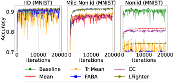
Figure 1: Classification accuracies of softmax regression on the MNIST dataset under static label flipping attacks.

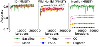
Figure 2: Classification accuracies of softmax regression on the MNIST dataset under dynamic label flipping attacks.

5.2 Convex Case

Classification accuracy. We consider softmax regression on the MNIST dataset. The classification accuracies under static label flipping and dynamic label flipping attacks are shown in Figure 1 and Figure 2, respectively. In the i.i.d. case, all methods perform well and close to the baseline. In the mild non-i.i.d. case, FABA and LFighter are the best among all aggregators and the other aggregators have similar performance. In the non-i.i.d. case, since the heterogeneity is large, all aggregators are tremendously affected by the label poisoning attacks, and have gaps to the baseline in terms of classification accuracy. Notably, the mean aggregator performs the best among all aggregators in this case, which validates our theoretical results.

Heterogeneity of regular local gradients and disturbance of poisoned local gradients. To further validate the reasonableness of Assumptions 3 and 4, as well as the correctness of our theoretical results in Section 4.1, we compute the smallest $\xi$ and $A$ that satisfy Assumptions 3 and 4 for the softmax regression problem. As shown in Figure 3, the disturbances of the poisoned local gradients, namely $A$, are bounded under both static label flipping and dynamic label flipping attacks, which corroborates the theoretical results in Lemma 1. From i.i.d., mild non-i.i.d. to the non-i.i.d. case, the heterogeneity of regular local gradients characterized by $\xi$ increases. Particularly, in the non-i.i.d. case, $\xi$ is close to $A$ under both static label flipping and dynamic label flipping attacks, which aligns our discussions below Lemma 2. Recall Table 1 that when the heterogeneity is sufficiently large, the learning error of the mean aggregator is optimal in order. This explains the results in Figures 1 and 2.

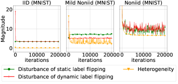
Figure 3: Heterogeneity of regular local gradients (the smallest $\xi$ satisfying Assumption 3) and disturbance of poisoned local gradients (the smallest $A$ satisfying Assumption 4) in softmax regression on the MNIST dataset, under static label flipping and dynamic label flipping attacks.

5.3 Nonconvex Case

Classification accuracy. Next, we train multi-layer perceptrons on the MNIST dataset and neural networks on the CIFAR10 dataset under static label flipping and dynamic label flipping attacks, as depicted in Figures 4 and 5. In the i.i.d. case, all methods have good performance and are close to the baseline, except for TriMean that performs worse than the other aggregators on the CIFAR10 dataset under dynamic label flipping attacks. In the mild non-i.i.d. case and on the MNIST dataset, Mean, FABA and LFighter are the best and close to the baseline, CC and TriMean perform worse, while TriMean is oscillating. On the CIFAR10 dataset, Mean, FABA, CC, and LFighter perform the best, while TriMean performs worse than the other methods with an obvious gap. In the non-i.i.d. case, all methods are affected by the attacks and cannot reach the same classification accuracy of the baseline, but mean aggregator still performs the best. CC, FABA and LFighter perform worse and TriMean fails.

Heterogeneity of regular local gradients and disturbance of poisoned local gradients. We also calculate the smallest values of $\xi$ and $A$ satisfying Assumptions 3 and 4, respectively. As shown in Figure 6, the disturbance of poisoned local gradients measured by $A$ are bounded on the MNIST and CIFAR10 datasets under both static label flipping and dynamic label flipping attacks. From i.i.d., mild non-i.i.d. to the non-i.i.d. case, the heterogeneity of regular local gradients $\xi$ is increasing. In the non-i.i.d. case, $\xi$ is close to $A$.

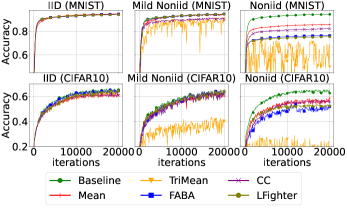
Figure 4: Classification accuracies of multi-layer perceptrons on the MNIST dataset and convolutional neural networks on the CIFAR10 dataset under static label flipping attacks.

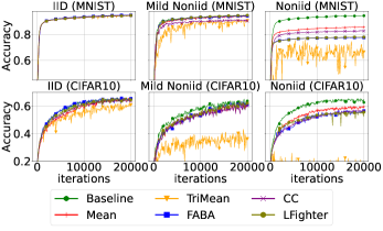
Figure 5: Classification accuracies of multi-layer perceptrons on the MNIST dataset and convolutional neural networks on the CIFAR10 dataset under dynamic label flipping attacks.

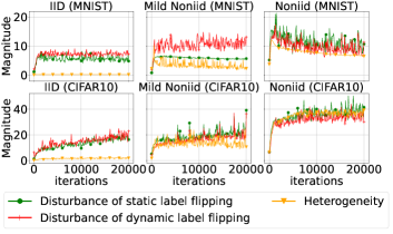
Figure 6: Heterogeneity of regular local gradients (the smallest $\xi$ satisfying Assumption 3) and disturbance of poisoned local gradients (the smallest $A$ satisfying Assumption 4) in training multi-layer perceptrons on the MNIST dataset and training convolutional neural networks on the CIFAR10 dataset, under static label flipping and dynamic label flipping attacks.

5.4 Impacts of Heterogeneity and Attack Strengths

To further show the impacts of heterogeneity of data distributions and strengths of label poisoning attacks, we compute classification accuracies of the trained multi-layer perceptrons neural network on the MNIST dataset, varying the data distributions and the levels of label poisoning attacks. We employ the Dirichlet distribution by varying the hyper-parameter $\alpha=\{100,1,0.1,0.001\}$ to simulate various heterogeneity of data distributions, in which a smaller $\alpha$ corresponds to larger heterogeneity. In addition, we let the poisoned worker apply static label flipping attacks by flipping labels with probability $p=\{0.0,0.4,0.7,1.0\}$ to simulate different attack strengths. A larger flipping probability indicates stronger attacks.

We present the best performance among all aggregators, and mark the corresponding best aggregator in Figure 7. The mean aggregator outperforms the robust aggregators when the heterogeneity is large. For example, the mean aggregator exhibits superior performance when $\alpha=0.001$ and the flipping probability $p=\{0,0.4,0.7,1.0\}$, as well as when $\alpha=0.1$ and $p=\{0,0.4,0.7\}$. Furthermore, fixing the flipping probability $p$, when the hyper-parameter $\alpha$ becomes smaller which means that the heterogeneity becomes larger, the mean aggregator gradually surpasses the robust aggregators. Fixing the hyper-parameter $\alpha$, when the flipping probability $p$ becomes smaller which means that the attack strength becomes smaller, the mean aggregator gradually surpasses the robust aggregators. According to the above observations, we recommend to apply the mean aggregator when the distributed data are sufficiently heterogeneous, or the disturbance caused by label poisoning attacks is comparable to the heterogeneity of regular local gradients.

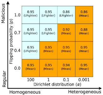
Figure 7: Best classification accuracies of trained multi-layer perceptrons by all aggregators on the MNIST dataset under static label flipping. Each block is associated with a hyper-parameter $\alpha$ that characterizes the heterogeneity and the flipping probability $p$ that characterizes the attack strength. For each block, the best classification accuracy and the corresponding aggregator is marked.

6 Conclusions

We studied the distributed learning problem subject to label poisoning attacks. We theoretically proved that when the distributed data are sufficiently heterogeneous, the learning error of the mean aggregator is optimal in order. Further corroborated by numerical experiments, our work revealed an important fact that state-of-the-art robust aggregators cannot always outperform the mean aggregator, if the attacks are confined to label poisoning. We expect that this fact can motivate us to revisit which application scenarios are proper for using robust aggregators. Our future work will extend the analysis to the more challenging decentralized learning problem.

Supplementary Material for
Mean Aggregator Is More Robust Than Robust Aggregators Under Label Poisoning Attacks

Appendix A A Analysis of distributed softmax regression

In this section, we analyze the property of distributed softmax regression where the local cost of worker $w\in\mathcal{W}$ is

$$\hat{f}_{w}(x)=-\frac{1}{J}\sum_{j=1}^{J}\sum_{k=1}^{K}\bm{1}\{b^{(w,j)}=k\}\log\frac{\exp(x_{k}^{T}a^{(w,j)})}{\sum_{l=1}^{K}\exp(x_{l}^{T}a^{(w,j)})}.$$ (16)

Here $K$ stands for the number of classes; $(a^{(w,j)},b^{(w,j)})$ represents the $j$-th sample of worker $w\in\mathcal{W}$ with $a^{(w,j)}\in{\mathbb{R}}^{d}$ and $b^{(w,j)}\in{\mathbb{R}}$ being the feature and the label, respectively; $\bm{1}\{b^{(w,j)}=k\}$ is the indicator function that outputs $1$ if $b^{(w,j)}=k$ and $0$ otherwise; $x_{k}\triangleq[x]_{kd:(k+1)d}\in{\mathbb{R}}^{d}$ is the $k$-th block of $x$. Note that $b^{(w,j)}$ for $w\in\mathcal{W}\setminus\mathcal{R}$ is probably mislabeled under label poisoning attacks.

We first show that the gradient of the local cost of worker $w\in\mathcal{W}$ is bounded in distributed softmax regression. Then we prove Lemma 1 which gives a valid constant $A$ to satisfy Assumption 4 in distributed softmax regression. Last, we prove Lemma 2 that gives the upper bound for the heterogeneity of the local costs $\xi$ in distributed softmax regression, and further demonstrate that when the distributed data across the regular workers are sufficiently heterogeneous, the constant $\xi$ is in the same order of $2\sqrt{K}\max_{w\in\mathcal{R}}\|\frac{1}{J}\sum_{j=1}^{J}a^{(w,j)}\|$.

A.1 Bounded gradients of local costs

Lemma 4.

Consider the distributed softmax regression problem where the local cost of worker $w\in\mathcal{W}$ is in the form of (16). Then the norm of the gradient of the local cost $\nabla\hat{f}_{w}(x)$ is bounded by the maximum of the norms of the local features, i.e.,

$$\|\nabla\hat{f}_{w}(x)\|\leq 2\max_{j\in[J]}\|a^{(w,j)}\|,\quad\forall w\in\mathcal{W}.$$ (17)

Moreover, if $a^{(w,j)}$ is entry-wise non-negative for all $w\in\mathcal{W}$ and all $j\in[J]$, we have

$$\|\nabla\hat{f}_{w}(x)\|\leq\sqrt{K}\|\frac{1}{J}\sum_{j=1}^{J}a^{(w,j)}\|,\quad\forall w\in\mathcal{W}.$$ (18)

Proof.

Note that $\hat{f}_{w}(x)=\frac{1}{J}\sum_{j=1}^{J}\hat{f}_{w,j}(x)$ where the sample cost function $\hat{f}_{w,j}(x)$ in distributed softmax regression is

$$\hat{f}_{w,j}(x)=-\sum_{k=1}^{K}\bm{1}\{b^{(w,j)}=k\}\log\frac{\exp(x_{k}^{T}a^{(w,j)})}{\sum_{l=1}^{K}\exp(x_{l}^{T}a^{(w,j)})}.$$ (19)

Therefore, the $k$-th block of the gradient of the sample cost function is

$$\nabla_{x_{k}}\hat{f}_{w,j}(x)=-a^{(w,j)}\big{(}\bm{1}\{b^{(w,j)}=k\}-\frac{\exp(x_{k}^{T}a^{(w,j)})}{\sum_{l=1}^{K}\exp(x_{l}^{T}a^{(w,j)})}\big{)}.$$ (20)

Taking the average of the gradients of the $J$ samples and concatenating the blocks together, we have

$$\|\nabla\hat{f}_{w}(x)\|^{2} =\sum_{k=1}^{K}\|\frac{1}{J}\sum_{j=1}^{J}\nabla_{x_{k}}\hat{f}_{w,j}(x)\|^{2}$$ (21)

$$=\sum_{k=1}^{K}\|\frac{1}{J}\sum_{j=1}^{J}a^{(w,j)}\big{(}\bm{1}\{b^{(w,j)}=k\}-\frac{\exp(x_{k}^{T}a^{(w,j)})}{\sum_{l=1}^{K}\exp(x_{l}^{T}a^{(w,j)})}\big{)}\|^{2}$$

$$\leq\sum_{k=1}^{K}\frac{1}{J}\sum_{j=1}^{J}\big{(}\bm{1}\{b^{(w,j)}=k\}-\frac{\exp(x_{k}^{T}a^{(w,j)})}{\sum_{l=1}^{K}\exp(x_{l}^{T}a^{(w,j)})}\big{)}^{2}\|a^{(w,j)}\|^{2},$$

where we use the inequality $\|\frac{1}{J}\sum_{j=1}^{J}v_{j}\|^{2}\leq\frac{1}{J}\sum_{j=1}^{J}\|v_{j}\|^{2}$ for any $J$ vectors $\{v_{j}\}_{j=1}^{J}$ in the last line. Since

$$\sum_{k=1}^{K}\Big{(}1\{b^{(w,j)}=k\}-\frac{\exp(x_{k}^{T}a^{(w,j)})}{\sum_{l=1}^{K}\exp(x_{l}^{T}a^{(w,j)})}\Big{)}^{2}\leq\Big{(}\sum_{k=1}^{K}|1\{b^{(w,j)}=k\}-\frac{\exp(x_{k}^{T}a^{(w,j)})}{\sum_{l=1}^{K}\exp(x_{l}^{T}a^{(w,j)})}|\Big{)}^{2}\leq 4,$$ (22)

we have

$$\|\nabla\hat{f}_{w}(x)\|^{2}\leq\frac{1}{J}\sum_{j=1}^{J}\sum_{k=1}^{K}\big{(}\bm{1}\{b^{(w,j)}=k\}-\frac{\exp(x_{k}^{T}a^{(w,j)})}{\sum_{l=1}^{K}\exp(x_{l}^{T}a^{(w,j)})}\big{)}^{2}\max_{j\in[J]}\|a^{(w,j)}\|^{2}\leq\big{(}2\max_{j\in[J]}\|a^{(w,j)}\|\big{)}^{2},$$ (23)

which shows the upper bound for the norm of the gradient.

Now, we turn to the second claim with the non-negativity assumption. Starting from the second equality in (21), we have

$$\|\nabla\hat{f}_{w}(x)\|^{2} =\sum_{k=1}^{K}\|\frac{1}{J}\sum_{j=1}^{J}a^{(w,j)}\big{(}\bm{1}\{b^{(w,j)}=k\}-\frac{\exp(x_{k}^{T}a^{(w,j)})}{\sum_{l=1}^{K}\exp(x_{l}^{T}a^{(w,j)})}\big{)}\|^{2}$$ (24)

$$\leq\sum_{k=1}^{K}\left\|\max_{j\in[J]}\big{|}\bm{1}\{b^{(w,j)}=k\}-\frac{\exp(x_{k}^{T}a^{(w,j)})}{\sum_{l=1}^{K}\exp(x_{l}^{T}a^{(w,j)})}\big{|}\cdot\frac{1}{J}\sum_{j=1}^{J}a^{(w,j)}\right\|^{2},$$

where the inequality is due to $\big{|}\sum_{j\in[J]}c_{j}x_{j}\big{|}\leq\max_{j\in[J]}|c_{j}|\cdot\sum_{j\in[J]}x_{j}$ for any sequence $\{c_{j}\}_{j\in[J]}$ and any positive sequence $\{x_{j}\}_{j\in[J]}$. Since $\max_{j\in[J]}\big{|}\bm{1}\{b^{(w,j)}=k\}-\frac{\exp(x_{k}^{T}a^{(w,j)})}{\sum_{l=1}^{K}\exp(x_{l}^{T}a^{(w,j)})}\big{|}\leq 1$, we reach our conclusion of

$$\|\nabla\hat{f}_{w}(x)\|^{2} \leq K\|\frac{1}{J}\sum_{j=1}^{J}a^{(w,j)}\|^{2},$$ (25)

which completes the proof.  

A.2 Proof of Lemma 1

We restate Lemma 1 as follows.

Lemma 5.

Consider the distributed softmax regression problem where the local cost is in the form of (9). The poisoned workers are under label poisoning attacks, with arbitrary fractions of sample labels being poisoned. If $a^{(w,j)}$ is entry-wise non-negative for all $w\in\mathcal{W}$ and all $j\in[J]$, then Assumption 4 is satisfied with

$$A=2\sqrt{K}\max_{w\in\mathcal{W}}\|\frac{1}{J}\sum_{j=1}^{J}a^{(w,j)}\|.$$ (26)

Proof.

Note that

$$\max_{w\in\mathcal{W}\setminus\mathcal{R}}\|\nabla\tilde{f}_{w}(x)-\nabla f(x)\|^{2}\leq 2\max_{w\in\mathcal{W}\setminus\mathcal{R}}\|\nabla\tilde{f}_{w}(x)\|^{2}+2\|\nabla f(x)\|^{2}.$$ (27)

From Lemma 4, we know the first term at the right-hand side of (27) can be upper-bounded as

$$\max_{w\in\mathcal{W}\setminus\mathcal{R}}\|\nabla\tilde{f}_{w}(x)\|^{2}\leq K\max_{w\in\mathcal{W}\setminus\mathcal{R}}\|\frac{1}{J}\sum_{j=1}^{J}a^{(w,j)}\|^{2}.$$ (28)

For the second term at the right-hand side of (27), applying the inequality $\|\frac{1}{R}\sum_{w\in\mathcal{R}}\nabla f_{w}\|^{2}\leq\frac{1}{R}\sum_{w\in\mathcal{R}}\|\nabla f_{w}\|^{2}$ gives

$$\|\nabla f(x)\|^{2}\leq\frac{1}{R}\sum_{w\in\mathcal{R}}\|\nabla f_{w}(x)\|^{2}\leq\max_{w\in\mathcal{R}}\|\nabla f_{w}(x)\|^{2}\leq K\max_{w\in\mathcal{R}}\|\frac{1}{J}\sum_{j=1}^{J}a^{(w,j)}\|^{2},$$ (29)

where the last inequality similarly comes from the assumption that $a^{(w,j)}$ is entry-wise non-negative for all $w\in\mathcal{W}$ and all $j\in[J]$.

Combining (28) and (29), we have

$$\max_{w\in\mathcal{W}\setminus\mathcal{R}}\|\nabla\tilde{f}_{w}(x)-\nabla f(x)\|^{2}\leq 4K\max_{w\in\mathcal{W}}\|\frac{1}{J}\sum_{j=1}^{J}a^{(w,j)}\|^{2},$$ (30)

or equivalently

$$\max_{w\in\mathcal{W}\setminus\mathcal{R}}\|\nabla\tilde{f}_{w}(x)-\nabla f(x)\|\leq 2\sqrt{K}\max_{w\in\mathcal{W}}\|\frac{1}{J}\sum_{j=1}^{J}a^{(w,j)}\|,$$ (31)

which is exactly (8) with $A=2\sqrt{K}\max_{w\in\mathcal{W}}\|\frac{1}{J}\sum_{j=1}^{J}a^{(w,j)}\|$.  

A.3 Proof of Lemma 2

We give a complete version of Lemma 2 as follows.

Lemma 6.

Consider the distributed softmax regression problem where the local cost is in the form of (9). The poisoned workers are under label poisoning attacks, with arbitrary fractions of sample labels being poisoned. If $a^{(w,j)}$ is entry-wise non-negative for all $w\in\mathcal{R}$ and all $j\in[J]$, then Assumption 3 is satisfied with

$$\xi\leq 2\sqrt{K}\max_{w\in\mathcal{R}}\|\frac{1}{J}\sum_{j=1}^{J}a^{(w,j)}\|.$$ (32)

On the other hand, suppose Assumption 3 holds true. If for any regular worker, the labels of its local data are the same and differ from labels of data at the other regular workers’ side (namely, $b^{(w,j)}=b^{(w^{\prime},j^{\prime})}$ if and only if $w=w^{\prime}$, for all $w,w^{\prime}\in\mathcal{R}$ and $j,j^{\prime}\in[j]$), we have

$$\xi=\Theta\big{(}\max_{w\in\mathcal{R}}\|\frac{1}{J}\sum_{j=1}^{J}a^{(w,j)}\|\big{)}.$$ (33)

Proof.

Notice that for any regular worker $w\in\mathcal{R}$, it holds

$$\|\nabla f_{w}(x)-\nabla f(x)\| =\|\big{(}1-\frac{1}{R}\big{)}\nabla f_{w}(x)-\sum_{w^{\prime}\in\mathcal{R},w^{\prime}\neq w}\frac{1}{R}\nabla f_{w^{\prime}}(x)\|$$ (34)

$$\leq\big{(}1-\frac{1}{R}\big{)}\|\nabla f_{w}(x)\|+\frac{1}{R}\sum_{w^{\prime}\in\mathcal{R},w^{\prime}\neq w}\|\nabla f_{w^{\prime}}(x)\|$$

$$\leq 2\max_{w^{\prime}\in\mathcal{R}}\|\nabla f_{w^{\prime}}(x)\|.$$

With (18) in Lemma 4, we have

$$\max_{w\in\mathcal{R}}\|\nabla f_{w}(x)-\nabla f(x)\|\leq 2\sqrt{K}\max_{w\in\mathcal{R}}\|\frac{1}{J}\sum_{j=1}^{J}a^{(w,j)}\|,$$ (35)

and thus Assumption 3 is satisfied with

$$\xi\leq 2\sqrt{K}\max_{w\in\mathcal{R}}\|\frac{1}{J}\sum_{j=1}^{J}a^{(w,j)}\|.$$ (36)

Next, we prove the lower bound of $\xi$. For any regular worker $w^{\prime}\in\mathcal{R}$ and any $x\in{\mathbb{R}}^{D}$, Assumption 3 gives that

$$\xi^{2}\geq\|\nabla f_{w^{\prime}}(x)-\nabla f(x)\|^{2}= \sum_{k=1}^{K}\|\frac{1}{J}\sum_{j=1}^{J}a^{(w^{\prime},j)}(\bm{1}\{b^{(w^{\prime},j)}=k\}-\frac{\exp(x_{k}^{T}a^{(w^{\prime},j)})}{\sum_{l=1}^{K}\exp(x_{l}^{T}a^{(w^{\prime},j)})})$$ (37)

$$-\frac{1}{R}\sum_{w\in\mathcal{R}}\frac{1}{J}\sum_{j=1}^{J}a^{(w,j)}(\bm{1}\{b^{(w,j)}=k\}-\frac{\exp(x_{k}^{T}a^{(w,j)})}{\sum_{l=1}^{K}\exp(x_{l}^{T}a^{(w,j)})})\|^{2}.$$

Letting $[x_{k}]_{i}=0$ for any $i\in[d]$ and $k\in[K]$, it holds that

$$\frac{\exp(x_{k}^{T}a^{(w,j)})}{\sum_{l=1}^{K}\exp(x_{l}^{T}a^{(w^{,}j)})}=\frac{1}{K},\quad\forall k\in[K],w\in\mathcal{R},j\in[J].$$

Given the heterogeneous label distribution, there exists $k^{\prime}\in[K]$, such that $b^{(w^{\prime},j)}=k^{\prime}\neq b^{(w,j)}$ for all $w\neq w^{\prime}$ and $j\in[J]$. Specifically, taking one of the summing parts in (37) with $k=k^{\prime}$, we obtain

$$\xi^{2}\geq \|\big{(}1-\frac{1}{R}\big{)}\frac{1}{J}\sum_{j=1}^{J}a^{(w^{\prime},j)}(1-\frac{1}{K})-\frac{1}{R}\sum_{w\in\mathcal{R},w\neq w^{\prime}}\frac{1}{J}\sum_{j=1}^{J}a^{(w,j)}(\bm{1}\{b^{(w,j)}=k^{\prime}\}-\frac{\exp(x_{k^{\prime}}^{T}a^{(w,j)})}{\sum_{l=1}^{K}\exp(x_{l}^{T}a^{(w,j)})})\|^{2}$$ (38)

$$= \|\big{(}1-\frac{1}{R}\big{)}\big{(}1-\frac{1}{K}\big{)}\frac{1}{J}\sum_{j=1}^{J}a^{(w^{\prime},j)}+\frac{1}{RK}\sum_{w\in\mathcal{R},w\neq w^{\prime}}\frac{1}{J}\sum_{j=1}^{J}a^{(w,j)}\|^{2}$$

$$\geq \|\big{(}1-\frac{1}{R}\big{)}\big{(}1-\frac{1}{K}\big{)}\frac{1}{J}\sum_{j=1}^{J}a^{(w^{\prime},j)}\|^{2},$$

where the last inequality is because each term in the summation is non-negative. Note that $w^{\prime}\in\mathcal{R}$ is arbitrary, which results in

$$\xi\geq\big{(}1-\frac{1}{R}\big{)}\big{(}1-\frac{1}{K}\big{)}\max_{w\in\mathcal{R}}\|\frac{1}{J}\sum_{j=1}^{J}a^{(w,j)}\|.$$ (39)

Combining (36) and (39), we have

$$\xi=\Theta\big{(}\max_{w\in\mathcal{R}}\|\frac{1}{J}\sum_{j=1}^{J}a^{(w,j)}\|\big{)},$$ (40)

which completes the proof.

 

Appendix B B Analysis of $\rho$-robust aggregators

In this section, we prove Lemma 3 that explores the approximation abilities of $\rho$-robust aggregators, and show that the state-of-the-art robust aggregators, including TriMean, CC, and FABA, are all $\rho$-robust aggregators when the fraction of poisoned workers is below their respective thresholds.

We first recall the definition of a $\rho$-robust aggregator.

Definition 3 ($\rho$-robust aggregator).

Consider any $W$ vectors $y_{1},y_{2},\ldots,y_{W}\in{\mathbb{R}}^{D}$, among which $R$ vectors are from regular workers $w\in\mathcal{R}$. An aggregator $\text{RAgg}(\cdot)$ is said to be a $\rho$-robust aggregator if there exists a contraction constant $\rho\geq 0$ such that

$$\|\text{RAgg}(\{y_{1},\ldots,y_{W}\})-\bar{y}\|\leq\rho\cdot\max_{w\in\mathcal{R}}\|y_{w}-\bar{y}\|,$$ (41)

where $\bar{y}=\frac{1}{R}\sum_{w\in\mathcal{R}}y_{w}$ is the average vector of the regular workers.

B.1 Proof of Lemma 3

The equivalent statement of Lemma 3 is shown below.

Lemma 7.

Denote $\delta\triangleq 1-\frac{R}{W}$ as the fraction of the poisoned workers. If $\delta\geq\frac{1}{2}$ or $\rho<\min\{\frac{\delta}{1-2\delta},1\}$, then there exist $W$ vectors $y_{1},y_{2},\ldots,y_{W}\in{\mathbb{R}}^{D}$ such that

$$\|\text{RAgg}(\{y_{1},\ldots,y_{W}\})-\bar{y}\|>\rho\cdot\max_{w\in\mathcal{R}}\|y_{w}-\bar{y}\|.$$ (42)

Proof.

Without loss of generality, consider $D=1$ and $\mathcal{R}=\{1,2,\ldots,R\}$. For higher-dimensional cases, setting all entries but one as zero will degenerate to the scalar case.

If $\delta\geq\frac{1}{2}$, then $2R\leq W$. Let $y_{1}=\ldots=y_{R}=0$, $y_{R+1}=\ldots y_{2R}=\rho+1$ and $y_{2R+1}=\ldots=y_{W}=0$. Then $\bar{y}=0$ and $\max_{w\in\mathcal{R}}\|y_{w}-\bar{y}\|=0$. If $\text{RAgg}(\{y_{1},\ldots,y_{W}\})\neq 0$, we have found $W$ vectors in (42). Otherwise, we know that $\text{RAgg}(\{y_{1},\ldots,y_{W}\})=0$. Rearranging those vectors as $z_{1}=\ldots z_{R}=\rho+1$ and $z_{R+1}=\ldots=z_{W}=0$, the aggregator based on the same set of vectors outputs the same value $\text{RAgg}(\{z_{1},\ldots,z_{W}\})=0$, while $\bar{z}=\rho+1$ and $\max_{w\in\mathcal{R}}\|z_{w}-\bar{z}\|=0$. Thus $\{z_{w},w\leq W\}$ are the set of vectors satisfying (42).

Next, consider $\delta<\frac{1}{2}$ but $\rho<\min\{\frac{\delta}{1-2\delta},1\}$. Similar to the above construction yet with $2R>W$, we consider $y_{1}=\ldots=y_{R}=0$ and $y_{R+1}=\ldots=y_{W}=1$. Accordingly, we have $\bar{y}=0$ and $\max_{w\in\mathcal{R}}\|y_{w}-\bar{y}\|=0$. If $\text{RAgg}(\{y_{1},\ldots,y_{W}\})\neq 0$, we have found $W$ vectors in (42). Otherwise, we get $\text{RAgg}(\{y_{1},\ldots,y_{W}\})=0$. Rearranging those vectors as $z_{1}=\ldots z_{W-R}=1$ and $z_{W-R+1}=\ldots=z_{W}=0$, the aggregator based on the same set of vectors outputs the same value $\text{RAgg}(\{z_{1},\ldots,z_{W}\})=0$, while $\bar{z}=\frac{\delta}{1-\delta}$ and $\max_{w\in\mathcal{R}}\|z_{w}-\bar{z}\|=\frac{\max\{1-2\delta,\delta\}}{1-\delta}$. Thus, $\{z_{w},w\leq W\}$ are the set of vectors satisfying (42).  

For notational convenience, hereafter we denote $\mathcal{P}$ as the set of poisoned workers, with $P=|\mathcal{P}|$ being the number of poisoned workers. Therefore, $\mathcal{P}=\mathcal{W}\setminus\mathcal{R}$ and $P=W-R$.

B.2 TriMean

TriMean is an aggregator that discards the smallest $P$ elements and largest $P$ elements in each dimension. The aggregated output of TriMean in dimension $d$ is given by

$$[\text{TriMean}(\{y_{1},\ldots,y_{W}\})]_{d}=\frac{1}{W-2P}\sum_{w\in[\mathcal{U}]_{d}}[y_{w}]_{d},$$ (43)

where $[\cdot]_{d}$ denotes the $d$-th coordinate of a vector, and $[\mathcal{U}]_{d}$ is the set of workers whose $d$-th elements are not filtered after removal. Below we show that TriMean is a $\rho$-robust aggregator if $\delta<\frac{1}{2}$.

Lemma 8.

Denote $\delta\triangleq 1-\frac{R}{W}$ as the fraction of the poisoned workers. If $\delta<\frac{1}{2}$, TriMean is a $\rho$-robust aggregator with $\rho=\frac{3\delta}{1-2\delta}\min\{\sqrt{D},\sqrt{R}\}$.

Proof.

We first analyze the aggregated result in one dimension $d$ and then extend it to all dimensions. Denote $[\mathcal{U}_{R}]_{d}\triangleq[\mathcal{U}]_{d}\cap\mathcal{R}$ and $[\mathcal{U}_{P}]_{d}\triangleq[\mathcal{U}]_{d}\cap\mathcal{P}$ as the set of remaining regular workers and poisoned workers after removal, respectively.

If TriMean successfully removes all the poisoned workers in dimension $d$, such that $[\mathcal{U}_{P}]_{d}=\emptyset$ and $[\mathcal{U}]_{d}\subseteq\mathcal{R}$, it holds

$$\|[\text{TriMean}(\{y_{1},\ldots,y_{W}\})]_{d}-[\bar{y}]_{d}\|= \|\frac{1}{W-2P}\sum_{w\in[\mathcal{U}]_{d}}[y_{w}]_{d}-\frac{1}{R}\sum_{w\in\mathcal{R}}[y_{w}]_{d}\|$$ (44)

$$= \|(\frac{1}{W-2P}-\frac{1}{R})\sum_{w\in\mathcal{R}}[y_{w}]_{d}-\frac{1}{W-2P}\sum_{w\in\mathcal{R}\setminus[\mathcal{U}]_{d}}[y_{w}]_{d}\|$$

$$= \|\frac{P}{W-2P}[\bar{y}]_{d}-\frac{1}{W-2P}\sum_{w\in\mathcal{R}\setminus[\mathcal{U}]_{d}}[y_{w}]_{d}\|$$

$$\leq \frac{1}{W-2P}\sum_{w\in\mathcal{R}\setminus[\mathcal{U}]_{d}}\|[y_{w}]_{d}-[\bar{y}]_{d}\|$$

$$\leq \frac{\delta}{1-2\delta}\cdot\max_{w\in\mathcal{R}}\|[y_{w}]_{d}-[\bar{y}]_{d}\|.$$

Otherwise, TriMean cannot remove all poisoned workers in dimension $d$, which means $[\mathcal{U}_{P}]_{d}\neq\emptyset$. Define

$$\bar{y}_{R_{d}}\triangleq\frac{1}{|[\mathcal{U}_{R}]_{d}|}\sum_{w\in[\mathcal{U}_{R}]_{d}}[y_{w}]_{d},\quad\bar{y}_{P_{d}}\triangleq\frac{1}{|[\mathcal{U}_{P}]_{d}|}\sum_{w\in[\mathcal{U}_{P}]_{d}}[y_{w}]_{d}$$ (45)

as the average of elements in $[\mathcal{U}_{R}]_{d}$ and $[\mathcal{U}_{P}]_{d}$, respectively. Also denote $u_{i}\triangleq\frac{|[\mathcal{U}_{P}]_{d}|}{|[\mathcal{U}]_{d}|}$ as the fraction of poisoned workers that remains. With the above definitions, we have $u_{i}\leq\frac{P}{W-2P}=\frac{\delta}{1-2\delta}$ and

$$\|[\text{TriMean}(\{y_{1},\ldots,y_{W}\})]_{d}-[\bar{y}]_{d}\|=\|u_{i}\cdot\bar{y}_{P_{d}}+(1-u_{i})\cdot\bar{y}_{R_{d}}-[\bar{y}]_{d}\|\leq u_{i}\|\bar{y}_{P_{d}}-[\bar{y}]_{d}\|+(1-u_{i})\|\bar{y}_{R_{d}}-[\bar{y}]_{d}\|.$$ (46)

For the first term at the right-hand side of (46), we have

$$u_{i}\|\bar{y}_{P_{d}}-[\bar{y}]_{d}\|= u_{i}\|\frac{1}{|[\mathcal{U}_{P}]_{d}|}\sum_{w\in[\mathcal{U}_{P}]_{d}}[y_{w}]_{d}-[\bar{y}]_{d}\|$$ (47)

$$\leq \frac{\delta}{1-2\delta}\max_{w\in[\mathcal{U}_{P}]_{d}}\|[y_{w}]_{d}-[\bar{y}]_{d}\|$$

$$\leq \frac{\delta}{1-2\delta}\max_{w\in\mathcal{R}}\|[y_{w}]_{d}-[\bar{y}]_{d}\|,$$

where the last inequality is due to the principle of filtering. Specifically, as the poisoned workers cannot own the $P$ largest values in dimension $d$, there exists a regular worker such that its $d$-th element is larger than $[y_{w}]_{d}$ for all $w\in[\mathcal{U}_{P}]_{d}$. Similarly, there exists a regular worker with the $d$-th element smaller than all $[y_{w}]_{d}$’s. This observation guarantees the last inequality in (47). For the second term at the right-hand side of (46), we have

$$(1-u_{i})\|\bar{y}_{R_{d}}-[\bar{y}]_{d}\|= (1-u_{i})\|(\frac{1}{|[\mathcal{U}_{R}]_{d}|}-\frac{1}{R})\sum_{w\in\mathcal{R}}[y_{w}]_{d}-\frac{1}{|[\mathcal{U}_{R}]_{d}|}\sum_{w\in\mathcal{R}\setminus[\mathcal{U}_{R}]_{d}}[y_{w}]_{d}\|$$ (48)

$$= (1-u_{i})\cdot\frac{1}{|[\mathcal{U}_{R}]_{d}|}\|\sum_{w\in\mathcal{R}\setminus[\mathcal{U}_{R}]_{d}}([y_{w}]_{d}-[\bar{y}]_{d})\|$$

$$\leq \frac{1}{W-2P}\sum_{w\in\mathcal{R}\setminus[\mathcal{U}_{R}]_{d}}\|[y_{w}]_{d}-[\bar{y}]_{d}\|$$

$$\leq \frac{R-|[\mathcal{U}_{R}]_{d}|}{W-2P}\max_{w\in\mathcal{R}}\|[y_{w}]_{d}-[\bar{y}]_{d}\|$$

$$\leq \frac{2\delta}{1-2\delta}\max_{w\in\mathcal{R}}\|[y_{w}]_{d}-[\bar{y}]_{d}\|,$$

where the last inequality is due to $|[\mathcal{U}_{R}]_{d}|=(W-2P)-|[\mathcal{U}_{P}]_{d}|\geq(W-2P)-P=R-2P$.

Substituting (47) and (48) into (46), we have

$$\|[\text{TriMean}(\{y_{1},\ldots,y_{W}\})]_{d}-[\bar{y}]_{d}\|\leq\frac{3\delta}{1-2\delta}\max_{w\in\mathcal{R}}\|[y_{w}]_{d}-[\bar{y}]_{d}\|.$$ (49)

Combining the first case (44) and the second case (49), we have

$$\|[\text{TriMean}(\{y_{1},\ldots,y_{W}\})]_{d}-[\bar{y}]_{d}\|\leq\frac{3\delta}{1-2\delta}\max_{w\in\mathcal{R}}\|[y_{w}]_{d}-[\bar{y}]_{d}\|.$$ (50)

Next, we extend the scalar scenario to the vector scenario. Notice that

$$\sum_{d=1}^{D}\max_{w\in\mathcal{R}}\|[y_{w}]_{d}-[\bar{y}]_{d}\|^{2}\leq\sum_{d=1}^{D}\max_{w\in\mathcal{R}}\|y_{w}-\bar{y}\|^{2}\leq D\max_{w\in\mathcal{R}}\|y_{w}-\bar{y}\|^{2}.$$ (51)

On the other hand, we also have

$$\sum_{d=1}^{D}\max_{w\in\mathcal{R}}\|[y_{w}]_{d}-[\bar{y}]_{d}\|^{2}\leq\sum_{d=1}^{D}\sum_{w\in\mathcal{R}}\|[y_{w}]_{d}-[\bar{y}]_{d}\|^{2}\leq\sum_{w\in\mathcal{R}}\sum_{d=1}^{D}\|[y_{w}]_{d}-[\bar{y}]_{d}\|^{2}\leq R\max_{w\in\mathcal{R}}\|y_{w}-\bar{y}\|^{2}.$$ (52)

Combining (51) and (52) gives

$$\sum_{d=1}^{D}\max_{w\in\mathcal{R}}\|[y_{w}]_{d}-[\bar{y}]_{d}\|^{2}\leq\min\{D,R\}\max_{w\in\mathcal{R}}\|y_{w}-\bar{y}\|^{2}.$$ (53)

Substituting (53) into (50), we have

$$\|\text{TriMean}(\{y_{1},\ldots,y_{W}\})-\bar{y}\|^{2}= \sum_{d=1}^{D}\|[\text{TriMean}(\{y_{1},\ldots,y_{W}\})]_{d}-[\bar{y}]_{d}\|^{2}$$ (54)

$$\leq (\frac{3\delta}{1-2\delta})^{2}\sum_{d=1}^{D}\max_{w\in\mathcal{R}}\|[y_{w}]_{d}-[\bar{y}]_{d}\|^{2}$$

$$\leq (\frac{3\delta}{1-2\delta})^{2}\min\{D,R\}\max_{w\in\mathcal{R}}\|y_{w}-\bar{y}\|^{2}.$$

Taking the square roots on both sides of (54), we have

$$\|\text{TriMean}(\{y_{1},\ldots,y_{W}\})-\bar{y}\|\leq\frac{3\delta}{1-2\delta}\cdot\min\{\sqrt{D},\sqrt{R}\}\cdot\max_{w\in\mathcal{R}}\|y_{w}-\bar{y}\|,$$ (55)

which completes the proof.  

B.3 CC

CC is an aggregator that iteratively clips the messages from workers. CC starts from some point $v^{0}$. At iteration $i$, the update rule of CC can be formulated as

$$v^{i+1}=v^{i}+\frac{1}{W}\sum_{w=1}^{W}\text{CLIP}(y_{w}-v^{i},\tau),$$ (56)

where

$$\text{CLIP}(y_{w}-v^{i},\tau)=\left\{\begin{aligned} &y_{w}-v^{i},&&\|y_{w}-v^{i}\|\leq\tau,\\ &\frac{\tau}{\|y_{w}-v^{i}\|}(y_{w}-v^{i}),&&\|y_{w}-v^{i}\|>\tau,\end{aligned}\right.$$ (57)

and $\tau\geq 0$ is the clipping threshold. After $L$ iterations, CC outputs the last vector as

$$\text{CC}(\{y_{1},\ldots,y_{W}\})=v^{L}.$$ (58)

Below we prove that with proper initialization and clipping threshold, one-step CC ($L=1$) is a $\rho$-robust aggregator if $\delta<\frac{1}{2}$.

Lemma 9.

Denote $\delta\triangleq 1-\frac{R}{W}$ as the fraction of the poisoned workers. If $\delta<\frac{1}{2}$, choosing the starting point $v_{0}$ satisfying $\|v_{0}-\bar{y}\|^{2}\leq\max_{w\in\mathcal{R}}\|y_{w}-\bar{y}\|^{2}$ and the clipping threshold $\tau=\sqrt{\frac{4(1-\delta)\max_{w\in\mathcal{R}}\|y_{w}-\bar{y}\|^{2}}{\delta}}$, one-step CC is a $\rho$-robust aggregator with $\rho=\sqrt{24\delta}$.

Proof.

The output of one-step CC is

$$\text{CC}(\{y_{1},\ldots,y_{W}\})=v^{0}+\frac{1}{W}\sum_{w=1}^{W}\text{CLIP}(y_{w}-v^{0},\tau).$$ (59)

Note that if $\max_{w\in\mathcal{R}}\|y_{w}-\bar{y}\|=0$, we have $\tau=0$ and $v^{0}=\bar{y}$, which leads to $\text{CC}(\{y_{1},\ldots,y_{W}\})=\bar{y}$. Therefore, we have

$$\|\text{CC}(\{y_{1},\ldots,y_{W}\})-\bar{y}\|=\max_{w\in\mathcal{R}}\|y_{w}-\bar{y}\|\leq\sqrt{24\delta}\max_{w\in\mathcal{R}}\|y_{w}-\bar{y}\|.$$ (60)

Below we consider the case that $\max_{w\in\mathcal{R}}\|y_{w}-\bar{y}\|>0$, then by definition $\tau>0$.

Denoting $\hat{y}_{w}=v^{0}+\text{CLIP}(y_{w}-v^{0},\tau)$ for any $w\in\{1,\ldots,W\}$, we have

$$\text{CC}(\{y_{1},\ldots,y_{W}\})=\frac{1}{W}\sum_{w=1}^{W}\hat{y}_{w}.$$ (61)

According to (61), we have

$$\|\text{CC}(\{y_{1},\ldots,y_{W}\})-\bar{y}\|^{2}= \|\frac{1}{W}\sum_{w=1}^{W}\hat{y}_{w}-\bar{y}\|^{2}$$ (62)

$$= \|(1-\delta)\cdot(\frac{1}{R}\sum_{w\in\mathcal{R}}\hat{y}_{w}-\bar{y})+\delta\cdot\frac{1}{P}\sum_{w\in\mathcal{P}}(\hat{y}_{w}-\bar{y})\|^{2}$$

$$\leq 2(1-\delta)^{2}\|\frac{1}{R}\sum_{w\in\mathcal{R}}(\hat{y}_{w}-y_{w})\|^{2}+2\delta^{2}\|\frac{1}{P}\sum_{w\in\mathcal{P}}(\hat{y}_{w}-\bar{y})\|^{2}$$

$$\leq 2(1-\delta)^{2}\frac{1}{R}\sum_{w\in\mathcal{R}}\|\hat{y}_{w}-y_{w}\|^{2}+2\delta^{2}\frac{1}{P}\sum_{w\in\mathcal{P}}\|\hat{y}_{w}-\bar{y}\|^{2}.$$

where the last two inequalities are due to the Cauchy-Schwarz inequality.

For any $w\in\mathcal{R}$, the term $\|\hat{y}_{w}-y_{w}\|$ holds

$$\|\hat{y}_{w}-y_{w}\|=v^{0}-y_{w}+\text{CLIP}(y_{w}-v^{0},\tau).$$ (63)

If the regular message $y_{w}$ is not clipped, meaning that $\text{CLIP}(y_{w}-v^{0},\tau)=y_{w}-v^{0}$, we have

$$\|\hat{y}_{w}-y_{w}\|=0.$$ (64)

Otherwise, we have

$$\|\hat{y}_{w}-y_{w}\|=\|v^{0}-y_{w}-\frac{\tau}{\|y_{w}-v^{l}\|}(v^{0}-y_{w})\|=\|v^{0}-y_{w}\|-\tau.$$ (65)

Since

$$\|v^{0}-y_{w}\|-\tau\leq\frac{\|v^{0}-y_{w}\|^{2}}{\tau}\leq\frac{2\|v^{0}-\bar{y}\|^{2}+2\|y_{w}-\bar{y}\|^{2}}{\tau}\leq\frac{4\max_{w\in\mathcal{R}}\|y_{w}-\bar{y}\|^{2}}{\tau},$$ (66)

where the first inequality is due to $a-b\leq\frac{a^{2}}{b}$ that holds for any $a\geq 0,b>0$, and the last inequality is due to $\|v_{0}-\bar{y}\|^{2}\leq\max_{w\in\mathcal{R}}\|y_{w}-\bar{y}\|^{2}$, we have

$$\|\hat{y}_{w}-y_{w}\|\leq\frac{4\max_{w\in\mathcal{R}}\|y_{w}-\bar{y}\|^{2}}{\tau}.$$ (67)

Combining (64) and (67), we have

$$\|\hat{y}_{w}-y_{w}\|\leq\frac{4\max_{w\in\mathcal{R}}\|y_{w}-\bar{y}\|^{2}}{\tau}.$$ (68)

For any $w\in\mathcal{P}$, the term $\|\hat{y}_{w}-\bar{y}\|^{2}$ holds

$$\|\hat{y}_{w}-\bar{y}\|^{2}\leq 2\|\hat{y}_{w}-v^{0}\|^{2}+2\|v^{0}-\bar{y}\|^{2}\leq 2\tau^{2}+2\max_{w\in\mathcal{R}}\|y_{w}-\bar{y}\|^{2},$$ (69)

where the last inequality is due to $\|\hat{y}_{w}-v^{0}\|^{2}=\|\text{CLIP}(y_{w}-v^{0},\tau)\|^{2}\leq\tau^{2}$ and $\|v_{0}-\bar{y}\|^{2}\leq\max_{w\in\mathcal{R}}\|y_{w}-\bar{y}\|^{2}$.

Substituting (68) and (69) into (62), we have

$$\|\text{CC}(\{y_{1},\ldots,y_{W}\})-\bar{y}\|^{2}$$ (70)

$$\leq 2(1-\delta)^{2}(\frac{4\max_{w\in\mathcal{R}}\|y_{w}-\bar{y}\|^{2}}{\tau})^{2}+4\delta^{2}\tau^{2}+4\delta^{2}\max_{w\in\mathcal{R}}\|y_{w}-\bar{y}\|^{2}$$

$$\leq 24\delta(1-\delta)\max_{w\in\mathcal{R}}\|y_{w}-\bar{y}\|^{2}+4\delta^{2}\max_{w\in\mathcal{R}}\|y_{w}-\bar{y}\|^{2}$$

$$\leq 24\delta\max_{w\in\mathcal{R}}\|y_{w}-\bar{y}\|^{2},$$

where the second inequality is due to $\tau=\sqrt{\frac{4(1-\delta)\max_{w\in\mathcal{R}}\|y_{w}-\bar{y}\|^{2}}{\delta}}$.

Therefore, we have

$$\|\text{CC}(\{y_{1},\ldots,y_{W}\})-\bar{y}\|\leq\sqrt{24\delta}\max_{w\in\mathcal{R}}\|y_{w}-\bar{y}\|.$$ (71)

Combining (60) and (71), we have that one-step CC is a $\rho$-robust aggregator with $\rho=\sqrt{24\delta}$. This completes the proof.  

B.4 FABA

FABA is an aggregator that iteratively discards a possible outlier and averages the messages that remain after $P$ iterations. To be more concrete, denote $\mathcal{U}^{(i)}$ as the set of workers that are not discarded at the $i$-th iteration. Initialized with $\mathcal{U}^{(0)}=\{1,\ldots,W\}$, at iteration $i$, FABA computes the average of the messages from $\mathcal{U}^{(i)}$ and discards the worker whose message is farthest from that average to form $\mathcal{U}^{(i+1)}$. After $P$ iterations, FABA obtains $\mathcal{U}^{(P)}$ with $W-P$ workers, and then outputs

$$\text{FABA}(\{y_{1},\ldots,y_{W}\})=\frac{1}{W-P}\sum_{w\in\mathcal{U}^{(P)}}y_{w}.$$ (72)

Below we prove that FABA is a $\rho$-robust aggregator if $\delta<\frac{1}{3}$.

Lemma 10.

Denote $\delta\triangleq 1-\frac{R}{W}$ as the fraction of poisoned workers. If $\delta<\frac{1}{3}$, FABA is a $\rho$-robust aggregator with $\rho=\frac{2\delta}{1-3\delta}$.

Proof.

For notational convenience, denote $\mathcal{R}^{(i)}\triangleq\mathcal{U}^{(i)}\cap\mathcal{R}$ and $\mathcal{P}^{(i)}\triangleq\mathcal{U}^{(i)}\cap\mathcal{P}$ as the sets of the regular workers and the poisoned workers in $\mathcal{U}^{(i)}$, respectively. Further denote three different averages

$$\bar{y}_{\mathcal{U}^{(i)}}\triangleq\frac{1}{|\mathcal{U}^{(i)}|}\sum_{w\in\mathcal{U}^{(i)}}y_{w},\quad\bar{y}_{\mathcal{R}^{(i)}}\triangleq\frac{1}{|\mathcal{R}^{(i)}|}\sum_{w\in\mathcal{R}^{(i)}}y_{w},\quad\bar{y}_{\mathcal{P}^{(i)}}\triangleq\frac{1}{|\mathcal{P}^{(i)}|}\sum_{w\in\mathcal{P}^{(i)}}y_{w}$$ (73)

over $\mathcal{U}^{(i)}$, $\mathcal{R}^{(i)}$ and $\mathcal{P}^{(i)}$, respectively. Then

$$\bar{y}_{\mathcal{U}^{(i)}}=(1-u_{i})\cdot\bar{y}_{\mathcal{R}^{(i)}}+u_{i}\cdot\bar{y}_{\mathcal{P}^{(i)}},$$ (74)

and our goal is to bound $\|\bar{y}_{\mathcal{U}^{(P)}}-\bar{y}\|$ by $\max_{w\in\mathcal{R}}\|y_{w}-\bar{y}\|$.

Denote $u_{i}\triangleq\frac{|\mathcal{P}^{(i)}|}{|\mathcal{U}^{(i)}|}$ as the fraction of the poisoned workers in $\mathcal{U}^{(i)}$. From $\delta<\frac{1}{3}$, $u_{i}\leq\frac{P}{W-P}<\frac{1}{2}$ for any $i\in\{0,\ldots,P\}$. We claim that a regular worker is filtered out at iteration $i$ only if

$$\|\bar{y}_{\mathcal{R}^{(i)}}-\bar{y}_{\mathcal{P}^{(i)}}\|\leq\frac{1}{1-2u_{i}}\max_{w\in\mathcal{R}}\|y_{w}-\bar{y}_{\mathcal{R}^{(i)}}\|.$$ (75)

This is because if $\|\bar{y}_{\mathcal{R}^{(i)}}-\bar{y}_{\mathcal{P}^{(i)}}\|>\frac{1}{1-2u_{i}}\max_{w\in\mathcal{R}}\|y_{w}-\bar{y}_{\mathcal{R}^{(i)}}\|$, then for any $w\in\mathcal{R}$, we have

$$\|y_{w}-\bar{y}_{\mathcal{U}^{(i)}}\|\leq \|y_{w}-\bar{y}_{\mathcal{R}^{(i)}}\|+\|\bar{y}_{\mathcal{R}^{(i)}}-\bar{y}_{\mathcal{U}^{(i)}}\|$$ (76)

$$= \|y_{w}-\bar{y}_{\mathcal{R}^{(i)}}\|+\frac{u_{i}}{1-u_{i}}\|\bar{y}_{\mathcal{P}^{(i)}}-\bar{y}_{\mathcal{U}^{(i)}}\|$$

$$\leq \max_{w\in\mathcal{R}}\|y_{w}-\bar{y}_{\mathcal{R}^{(i)}}\|+\frac{u_{i}}{1-u_{i}}\|\bar{y}_{\mathcal{P}^{(i)}}-\bar{y}_{\mathcal{U}^{(i)}}\|$$

$$< \frac{1-2u_{i}}{1-u_{i}}\|\bar{y}_{\mathcal{P}^{(i)}}-\bar{y}_{\mathcal{U}^{(i)}}\|+\frac{u_{i}}{1-u_{i}}\|\bar{y}_{\mathcal{P}^{(i)}}-\bar{y}_{\mathcal{U}^{(i)}}\|$$

$$\leq \max_{w\in\mathcal{P}^{(i)}}\|y_{w}-\bar{y}_{\mathcal{U}^{(i)}}\|,$$

where (74) is applied to both the second and fourth lines. Therefore, there exists $w^{\prime}\in\mathcal{P}^{(i)}$ with farther distance to $\bar{y}_{\mathcal{U}^{(i)}}$ than all the regular workers, which guarantees that all the remaining regular workers will not be removed in this iteration.

If at every iteration FABA discards a poisoned worker, then $\mathcal{U}^{(P)}=\mathcal{R}$ and

$$\|\bar{y}_{\mathcal{U}^{(P)}}-\bar{y}\|=0\leq\frac{2\delta}{1-3\delta}\cdot\max_{w\in\mathcal{R}}\|y_{w}-\bar{y}\|.$$ (77)

Otherwise, there are iterations with regular workers removed. Denote $i^{*}$ as the last one among the $P$ iterations that removes the regular worker. Denote $w^{(i^{*})}$ as the discarded worker at iteration $i^{*}$, we have $w^{(i^{*})}\in\mathcal{R}$ and from the algorithmic principle of removal

$$\|y_{w^{(i^{*})}}-\bar{y}_{\mathcal{U}^{(i^{*})}}\|=\max_{w\in\mathcal{U}^{(i^{*})}}\|y_{w}-\bar{y}_{\mathcal{U}^{(i^{*})}}\|.$$ (78)

Note that

$$\|\bar{y}_{\mathcal{U}^{(P)}}-\bar{y}\|\leq\|\bar{y}_{\mathcal{U}^{(P)}}-\bar{y}_{\mathcal{U}^{(i^{*})}}\|+\|\bar{y}_{\mathcal{U}^{(i^{*})}}-\bar{y}\|,$$ (79)

thus it suffices to bound the two terms on the right separately. First we notice that

$$\|\bar{y}_{\mathcal{U}^{(P)}}-\bar{y}_{\mathcal{U}^{(i^{*})}}\|= \|\frac{1}{|\mathcal{U}^{(P)}|}\sum_{w\in\mathcal{U}^{(P)}}y_{w}-\frac{1}{|\mathcal{U}^{(i^{*})}|}\sum_{w\in\mathcal{U}^{(i^{*})}}y_{w}\|$$ (80)

$$= \|(\frac{1}{|\mathcal{U}^{(P)}|}-\frac{1}{|\mathcal{U}^{(i^{*})}|})\sum_{w\in\mathcal{U}^{(i^{*})}}y_{w}-\frac{1}{|\mathcal{U}^{(P)}|}\sum_{w\in\mathcal{U}^{(i^{*})}\setminus\mathcal{U}^{(P)}}y_{w}\|$$

$$= \frac{1}{|\mathcal{U}^{(P)}|}\|\sum_{w\in\mathcal{U}^{(i^{*})}\setminus\mathcal{U}^{(P)}}(y_{w}-\bar{y}_{\mathcal{U}^{(i^{*})}})\|$$

$$\leq \frac{|\mathcal{U}^{(i^{*})}|-|\mathcal{U}^{(P)}|}{|\mathcal{U}^{(P)}|}\max_{w\in\mathcal{U}^{(i^{*})}\setminus\mathcal{U}^{(P)}}\|y_{w}-\bar{y}_{\mathcal{U}^{(i^{*})}}\|$$

$$\leq \frac{P-i^{*}}{R}\|y_{w^{(i^{*})}}-\bar{y}_{\mathcal{U}^{(i^{*})}}\|$$

$$\leq \frac{P-i^{*}}{R}(\|y_{w^{(i^{*})}}-\bar{y}_{\mathcal{R}^{(i^{*})}}\|+\|\bar{y}_{\mathcal{R}^{(i^{*})}}-\bar{y}_{\mathcal{U}^{(i^{*})}}\|)$$

$$= \frac{P-i^{*}}{R}(\|y_{w^{(i^{*})}}-\bar{y}_{\mathcal{R}^{(i^{*})}}\|+u_{i^{*}}\|\bar{y}_{\mathcal{R}^{(i^{*})}}-\bar{y}_{\mathcal{P}^{(i^{*})}}\|)$$

$$\leq \frac{P-i^{*}}{R}\left(\max_{w\in\mathcal{R}}\|y_{w}-\bar{y}_{\mathcal{R}^{(i^{*})}}\|+\frac{u_{i^{*}}}{1-2u_{i^{*}}}\cdot\max_{w\in\mathcal{R}}\|y_{w}-\bar{y}_{\mathcal{R}^{(i^{*})}}\|\right)$$

$$= \frac{P-i^{*}}{R}\cdot\frac{1-u_{i^{*}}}{1-2u_{i^{*}}}\max_{w\in\mathcal{R}}\|y_{w}-\bar{y}_{\mathcal{R}^{(i^{*})}}\|,$$

where the second inequality is from (78) and the last inequality is from (75) with $i=i^{*}$. Additionally, the second term at the right-hand side of (79) has upper bound

$$\|\bar{y}_{\mathcal{U}^{(i^{*})}}-\bar{y}\|=\|(1-u_{i^{*}})\cdot\bar{y}_{\mathcal{R}^{(i^{*})}}+u_{i^{*}}\cdot\bar{y}_{\mathcal{P}^{(i^{*})}}-\bar{y}\|\leq\|\bar{y}_{\mathcal{R}^{(i^{*})}}-\bar{y}\|+u_{i^{*}}\|\bar{y}_{\mathcal{R}^{(i^{*})}}-\bar{y}_{\mathcal{P}^{(i^{*})}}\|.$$ (81)

For $\|\bar{y}_{\mathcal{R}^{(i^{*})}}-\bar{y}\|$, we have

$$\|\bar{y}_{\mathcal{R}^{(i^{*})}}-\bar{y}\|= \|\frac{1}{|\mathcal{R}^{(i^{*})}|}\sum_{w\in\mathcal{R}^{(i^{*})}}y_{w}-\frac{1}{R}\sum_{w\in\mathcal{R}}y_{w}\|$$ (82)

$$= \frac{1}{|\mathcal{R}^{(i^{*})}|}\|\sum_{w\in\mathcal{R}\setminus\mathcal{R}^{i^{*}}}(\bar{y}-y_{w})\|$$

$$\leq \frac{R-|\mathcal{R}^{(i^{*})}|}{|\mathcal{R}^{(i^{*})}|}\max_{w\in\mathcal{R}}\|y_{w}-\bar{y}\|.$$

Substituting (82) and (75) into (81), we have

$$\|\bar{y}_{\mathcal{U}^{(i^{*})}}-\bar{y}\|\leq\frac{R-|\mathcal{R}^{(i^{*})}|}{|\mathcal{R}^{(i^{*})}|}\max_{w\in\mathcal{R}}\|y_{w}-\bar{y}\|+\frac{u_{i^{*}}}{1-2u_{i^{*}}}\max_{w\in\mathcal{R}}\|y_{w}-\bar{y}_{\mathcal{R}^{(i^{*})}}\|.$$ (83)

Substituting (80) and (83) into (79), we have

$$\|\bar{y}_{\mathcal{U}^{(P)}}-\bar{y}\|\leq(\frac{P-i^{*}}{R}\cdot\frac{1-u_{i^{*}}}{1-2u_{i^{*}}}+\frac{u_{i^{*}}}{1-2u_{i^{*}}})\max_{w\in\mathcal{R}}\|y_{w}-\bar{y}_{\mathcal{R}^{(i^{*})}}\|+\frac{R-|\mathcal{R}^{(i^{*})}|}{|\mathcal{R}^{(i^{*})}|}\max_{w\in\mathcal{R}}\|y_{w}-\bar{y}\|.$$ (84)

Since

$$\max_{w\in\mathcal{R}}\|y_{w}-\bar{y}_{\mathcal{R}^{(i^{*})}}\|\leq\max_{w\in\mathcal{R}}\|y_{w}-\bar{y}\|+\|\bar{y}_{\mathcal{R}^{(i^{*})}}-\bar{y}\|\leq\frac{R}{|\mathcal{R}^{(i^{*})}|}\max_{w\in\mathcal{R}}\|y_{w}-\bar{y}\|,$$ (85)

where the last inequality comes from (82), we have

$$\|\bar{y}_{\mathcal{U}^{(P)}}-\bar{y}\|\leq\Big{(}(\frac{P-i^{*}}{R}\cdot\frac{1-u_{i^{*}}}{1-2u_{i^{*}}}+\frac{u_{i^{*}}}{1-2u_{i^{*}}})\frac{R}{|\mathcal{R}^{(i^{*})}|}+\frac{R-|\mathcal{R}^{(i^{*})}|}{|\mathcal{R}^{(i^{*})}|}\Big{)}\max_{w\in\mathcal{R}}\|y_{w}-\bar{y}\|=\frac{2u_{i^{*}}}{1-2u_{i^{*}}}\max_{w\in\mathcal{R}}\|y_{w}-\bar{y}\|.$$ (86)

Since $u_{i^{*}}=\frac{|\mathcal{P}^{(i^{*})}|}{|\mathcal{U}^{(i^{*})}|}\leq\frac{P}{R}=\frac{\delta}{1-\delta}$, we have

$$\|\bar{y}_{\mathcal{U}^{(P)}}-\bar{y}\|\leq\frac{2\delta}{1-3\delta}\cdot\max_{w\in\mathcal{R}}\|y_{w}-\bar{y}\|.$$ (87)

Combining the first case (77) and the second case (87), we have

$$\|\text{FABA}(\{y_{1},\ldots,y_{W}\}-\bar{y})\|=\|\bar{y}_{\mathcal{U}^{(P)}}-\bar{y}\|\leq\frac{2\delta}{1-3\delta}\cdot\max_{w\in\mathcal{R}}\|y_{w}-\bar{y}\|,$$ (88)

which completes the proof.

 

Appendix C C Proof of Theorem 1

We restate Theorem 1 as follows.

Theorem 4.

Consider Algorithm 1 with a $\rho$-robust aggregator $\text{RAgg}(\cdot)$ to solve (1). Under label poisoning attacks where the fraction of poisoned workers is $\delta\in[0,\frac{1}{2})$, if the step size is $\gamma\in(0,\frac{1}{L}]$ and Assumptions 1, 2 and 3 are satisfied, then we have

$$\|\nabla f(\hat{x})\|^{2}\leq\frac{8(f(x^{0})-f^{*})}{\gamma T}+10\rho^{2}\xi^{2}.$$ (89)

Proof.

For notational simplicity, denote $g^{t}=\text{RAgg}(\{\nabla\hat{f}_{w}(x^{t}):w\in\mathcal{W}\})$. Since $f(x)$ has $L$-Lipschitz continuous gradients from Assumption 2, it holds that

$$f(x^{t+1})\leq f(x^{t})+\langle\nabla f(x^{t}),x^{t+1}-x^{t}\rangle+\frac{L}{2}\|x^{t+1}-x^{t}\|^{2}$$ (90)

$$\leq f(x^{t})-\gamma\langle\nabla f(x^{t}),g^{t}\rangle+\frac{L}{2}\gamma^{2}\|g^{t}\|^{2}.$$

Since

$$-\langle\nabla f(x^{t}),g^{t}\rangle=\frac{1}{2}\|g^{t}-\nabla f(x^{t})\|^{2}-\frac{1}{2}\|\nabla f(x^{t})\|^{2}-\frac{1}{2}\|g^{t}\|^{2},$$ (91)

we have

$$f(x^{t+1})\leq f(x^{t})+\frac{\gamma}{2}\|g^{t}-\nabla f(x^{t})\|^{2}-\frac{\gamma}{2}\|\nabla f(x^{t})\|^{2}-\frac{\gamma}{2}(1-L\gamma)\|g^{t}\|^{2}$$ (92)

$$\leq f(x^{t})+\frac{\gamma}{2}\|g^{t}-\nabla f(x^{t})\|^{2}-\frac{\gamma}{2}\|\nabla f(x^{t})\|^{2},$$

where the last inequality is from $\gamma\in(0,\frac{1}{L}]$. Further, since $\text{RAgg}(\cdot)$ is a $\rho$-robust aggregator with definition (41), it holds that

$$\|g^{t}-\nabla f(x^{t})\|^{2}\leq\rho^{2}\max_{w\in\mathcal{R}}\|\nabla f_{w}(x^{t})-\nabla f(x^{t})\|^{2}\leq\rho^{2}\xi^{2},$$ (93)

where the last inequality comes from Assumption 3. Substituting (93) into (92), we have

$$\|\nabla f(x^{t})\|^{2}\leq\frac{2(f(x^{t})-f(x^{t+1}))}{\gamma}+\rho^{2}\xi^{2}.$$ (94)

Taking the average over $t$ from $0$ to $T-1$, we have

$$\frac{1}{T}\sum_{t=0}^{T-1}\|\nabla f(x^{t})\|^{2}\leq\frac{2(f(x^{0})-f(x^{T}))}{\gamma T}+\rho^{2}\xi^{2}\leq\frac{2(f(x^{0})-f^{*})}{\gamma T}+\rho^{2}\xi^{2},$$ (95)

where the last inequality comes from Assumption 1 such that $f(x^{T})\geq f^{*}$.

Recall that the output $\hat{x}$ of Algorithm 1 is $\hat{x}=x^{\tau}$ where $\tau\in\arg\min_{0\leq t\leq T-1}\|g^{t}\|$. Our goal is to bound

$$\|\nabla f(\hat{x})\|^{2}=\|\nabla f(x^{\tau})\|^{2}=\|\nabla f(x^{\tau})-g^{\tau}+g^{\tau}\|^{2}\leq 2\|\nabla f(x^{\tau})-g^{\tau}\|^{2}+2\|g^{\tau}\|^{2}.$$ (96)

According to (93), we have $\|\nabla f(x^{\tau})-g^{\tau}\|^{2}\leq\rho^{2}\xi^{2}$ and further

$$\|g^{\tau}\|^{2}=\min_{0\leq t\leq T-1}\|g^{t}\|^{2}\leq \min_{0\leq t\leq T-1}\{\|\nabla f(x^{t})+g^{t}-\nabla f(x^{t})\|^{2}\}$$ (97)

$$\leq \min_{0\leq t\leq T-1}\{2\|\nabla f(x^{t})\|^{2}+2\|g^{t}-\nabla f(x^{t})\|^{2}\}$$

$$\leq \min_{0\leq t\leq T-1}\{2\|\nabla f(x^{t})\|^{2}\}+2\rho^{2}\xi^{2}$$

$$\leq \frac{2}{T}\sum_{t=0}^{T-1}\|\nabla f(x^{t})\|^{2}+2\rho^{2}\xi^{2}$$

$$\leq \frac{4(f(x^{0})-f^{*})}{\gamma T}+4\rho^{2}\xi^{2}.$$

As a result, we have

$$\|\nabla f(\hat{x})\|^{2}\leq\frac{8(f(x^{0})-f^{*})}{\gamma T}+10\rho^{2}\xi^{2},$$ (98)

which completes the proof.  

Appendix D D Proof of Theorem 2

We restate Theorem 2 as follows.

Theorem 5.

Consider Algorithm 1 with the mean aggregator $\text{Mean}(\cdot)$ to solve (1). Under label poisoning attacks where the fraction of poisoned workers is $\delta\in[0,1)$, if the step size is $\gamma\in(0,\frac{1}{L}]$ and Assumptions 1, 2 and 4 are satisfied, then we have

$$\|\nabla f(\hat{x})\|^{2}\leq\frac{8(f(x^{0})-f^{*})}{\gamma T}+10\delta^{2}A^{2}.$$ (99)

Proof.

For notational simplicity, denote $g^{t}=\text{Mean}(\{\nabla\hat{f}_{w}(x^{t}):w\in\mathcal{W}\})$. Note that the same inequality (92) holds true with Assumption 2, which says

$$f(x^{t+1})\leq f(x^{t})+\frac{\gamma}{2}\|g^{t}-\nabla f(x^{t})\|^{2}-\frac{\gamma}{2}\|\nabla f(x^{t})\|^{2}.$$ (100)

For the term $\|g^{t}-\nabla f(x^{t})\|^{2}$, we have

$$\|g^{t}-\nabla f(x^{t})\|^{2} =\|\frac{1}{W}\sum_{w\in\mathcal{W}}\nabla\hat{f}_{w}(x^{t})-\nabla f(x^{t})\|^{2}$$ (101)

$$=\|\frac{1}{W}\sum_{w\in\mathcal{W}\setminus\mathcal{R}}\nabla\tilde{f}_{w}(x^{t})+\frac{R}{W}\nabla f(x^{t})-\nabla f(x^{t})\|^{2}$$

$$=\|\frac{1}{W}\sum_{w\in\mathcal{W}\setminus\mathcal{R}}\big{(}\nabla\tilde{f}_{w}(x^{t})-\nabla f(x^{t})\big{)}\|^{2}$$

$$\leq\frac{1}{W^{2}}\bigg{(}\sum_{w\in\mathcal{W}\setminus\mathcal{R}}\|\nabla\tilde{f}_{w}(x^{t})-\nabla f(x^{t})\|\bigg{)}^{2}$$

$$\leq\frac{(W-R)^{2}}{W^{2}}\max_{w\in\mathcal{W}\setminus\mathcal{R}}\|\nabla\tilde{f}_{w}(x^{t})-\nabla f(x^{t})\|^{2}$$

$$\leq\delta^{2}A^{2},$$

where the last inequality comes from Assumption 4.

Substituting (101) into (100) gives

$$\|\nabla f(x^{t})\|^{2}\leq\frac{2(f(x^{t})-f(x^{t+1}))}{\gamma}+\delta^{2}A^{2}.$$ (102)

Taking the average over $t$ from $0$ to $T-1$, we have

$$\frac{1}{T}\sum_{t=0}^{T-1}\|\nabla f(x^{t})\|^{2}\leq\frac{2(f(x^{0})-f(x^{T}))}{\gamma T}+\delta^{2}A^{2}\leq\frac{2(f(x^{0})-f^{*})}{\gamma T}+\delta^{2}A^{2},$$ (103)

where the last inequality comes from Assumption 1 such that $f(x^{T})\geq f^{*}$.

With (101) and (103), the rest of the proof follows that of Theorem 1 from (96) to (98) by replacing $\rho^{2}\xi^{2}$ with $\delta^{2}A^{2}$, and is therefore omitted.  

Appendix E E Proof of Theorem 3

We recall the statement of Theorem 3 as follows.

Theorem 6.

Under label poisoning attacks with $\delta=1-\frac{R}{W}$ fraction of poisoned workers, consider Algorithm 1 with any $\rho$-robust aggregator or the mean aggregator, where $\rho\geq\min\{\frac{\delta}{1-2\delta},1\}$. There exist $R$ regular local functions $\{f_{w}(x):{w\in\mathcal{R}}\}$ and $W-R$ poisoned local functions $\{\tilde{f}_{w}(x):{w\in\mathcal{W}\setminus\mathcal{R}}\}$ satisfying Assumptions 1, 2 , 3 and 4 such that the output $\hat{x}$ of Algorithm 1 has

$$\|\nabla f(\hat{x})\|^{2}\geq\Omega(\delta^{2}\xi^{2}).$$ (104)

Proof.

The key idea of the proof is to find two sets of $W$ local costs that are the same under label poisoning attacks, while their objectives based on $R$ regular local costs are different. Therefore Algorithm 1 with any $\rho$-robust aggregator or the mean aggregator cannot distinguish between them and the algorithmic output necessarily has an error on at least one of the two tasks.

The construction of the example is as follows. Without loss of generality, let $\mathcal{W}=\{1,\ldots,W\}$ be the set of workers where $\mathcal{R}=\{1,\ldots,R\}$ is the set of regular workers. The data among all workers have two possible labels, $1$ or $2$. Consider two different functions $f(x;1)$ and $f(x;2)$ where

$$f(x;k)=\frac{(1-\delta)\xi}{\sqrt{2}}[x]_{k}+\frac{L}{2}\|x\|^{2},\quad k\in\{1,2\}.$$ (105)

For each worker $w\in[W]$, there is only one data with label $b^{(w)}$. The two different sets of local costs share the same form of

$$f_{w}(x) =f(x;b^{(w)}),\quad\forall w\leq R,$$ (106)

$$\tilde{f}_{w}(x) =f(x;b^{(w)}),\quad\forall w>R.$$ (107)

However, the labels differ. The first set of labels, denoted as $\{b^{(w,1)},w\in[W]\}$, consists of

$$b^{(w,1)}=\begin{cases}1,&w\leq R,\\ 2,&w>R,\end{cases}$$ (108)

while the second set with notation $\{b^{(w,2)},w\in[W]\}$ is defined as

$$b^{(w,2)}=\begin{cases}1,&w>W-R,\\ 2,&w\leq W-R.\end{cases}$$ (109)

The above two settings result in the same set of local costs ($R$ of them are $f(x;1)$ and the others are $f(x;2)$) yet different orders of labels. In particular, if we denote $f^{(1)}(x)=\frac{1}{R}\sum_{w=1}^{R}f(x;b^{(w,1)})$ and $f^{(2)}=\frac{1}{R}\sum_{w=1}^{R}f(x;b^{(w,2)})$ as the two objectives, we can check that all the assumptions are satisfied by both, and the learning error of an algorithmic output has a non-vanishing lower bound on one of the objectives. Since

$$\nabla f(x;k) =\frac{(1-\delta)\xi}{\sqrt{2}}e_{k}+Lx,$$ (110)

where $e_{k}$ is the unit vector with the $k$-th element being $1$, we obtain the gradients of $f^{(1)}$ and $f^{(2)}$ are

$$\nabla f^{(1)}(x) =\frac{(1-\delta)\xi}{\sqrt{2}}e_{1}+Lx,$$ (111)

$$\nabla f^{(2)}(x) =\frac{(1-2\delta)\xi}{\sqrt{2}}e_{1}+\frac{\delta\xi}{\sqrt{2}}e_{2}+Lx.$$ (112)

As a result, we know their minimums are achieved at $x^{*,(1)}=-\frac{(1-\delta)\xi}{\sqrt{2}L}e_{1}$ and $x^{*,(2)}=-\frac{(1-2\delta)\xi}{\sqrt{2}L}e_{1}-\frac{\delta\xi}{\sqrt{2}L}e_{2}$, respectively, and there exists a uniform lower bound

$$f^{(k)}(x)\geq f^{*}\triangleq-\frac{\xi^{2}}{2L}$$ (113)

satisfying Assumption 1. As the gradients are linear, Assumption 2 is satisfied with $L$. Further, Assumption 3 is satisfied with constant $\xi$, as

$$\max_{w\leq R}\|\nabla f(x;b^{(w,1)})-\nabla f^{(1)}(x)\|=0,\quad\max_{w\leq R}\|\nabla f(x;b^{(w,2)})-\nabla f^{(2)}(x)\|=\max\{|1-2\delta|,\delta\}\xi\leq\xi.$$ (114)

Assumption 4 is analogously satisfied with $A=\max\{\delta,(1-\delta)\}\xi$, since

$$\max_{w>R}\|\nabla f(x;b^{(w,1)})-\nabla f^{(1)}(x)\|=(1-\delta)\xi,\quad\max_{w>R}\|\nabla f(x;b^{(w,2)})-\nabla f^{(2)}(x)\|=\delta\xi.$$ (115)

For any $x$, we notice that

$$\max\{\|\nabla f^{(1)}(x)\|,\|\nabla f^{(2)}(x)\|\}\geq\frac{1}{2}\left(\|\nabla f^{(1)}(x)\|+\|\nabla f^{(2)}(x)\|\right)\geq\frac{1}{2}\|\nabla f^{(1)}(x)-\nabla f^{(2)}(x)\|=\frac{\delta\xi}{2}.$$ (116)

Specifically let $x=\hat{x}$ be the output of Algorithm 1 with any $\rho$-robust aggregator or the mean aggregator running on either one of the two settings. Choosing $R$ regular local functions $\{f_{w}(x)=f(x;b^{(w,k)}):w\leq R\}$ and $W-R$ poisoned local functions $\{\tilde{f}_{w}(x)=f(x;b^{(w,k)}):w>R\}$ where $k=\operatorname*{arg\,max}_{k\in\{1,2\}}\|\nabla f^{(k)}(\hat{x})\|$, (116) gives that

$$\|\nabla f(\hat{x})\|^{2}\geq\frac{\delta^{2}\xi^{2}}{4}=\Omega(\delta^{2}\xi^{2}),$$ (117)

which concludes the proof.

References

• Allouah et al. [2023] Youssef Allouah, Sadegh Farhadkhani, Rachid Guerraoui, Nirupam Gupta, Rafaël Pinot, and John Stephan. Fixing by mixing: a recipe for optimal Byzantine ML under heterogeneity. In International Conference on Artificial Intelligence and Statistics, pages 1232–1300, 2023.
• Bagdasaryan et al. [2020] Eugene Bagdasaryan, Andreas Veit, Yiqing Hua, Deborah Estrin, and Vitaly Shmatikov. How to backdoor federated learning. In International Conference on Artificial Intelligence and Statistics, pages 2938–2948, 2020.
• Blanchard et al. [2017] Peva Blanchard, El Mahdi El Mhamdi, Rachid Guerraoui, and Julien Stainer. Machine learning with adversaries: Byzantine tolerant gradient descent. In Advances in Neural Information Processing Systems, pages 118–128, 2017.
• Carmon et al. [2020] Yair Carmon, John C. Duchi, Oliver Hinder, and Aaron Sidford. Lower bounds for finding stationary points i. Mathematical Programming, 184(1–2):71–120, 2020.
• Chen et al. [2017] Yudong Chen, Lili Su, and Jiaming Xu. Distributed statistical machine learning in adversarial settings: Byzantine gradient descent. ACM on Measurement and Analysis of Computing Systems, 1(2):1–25, 2017.
• Dong et al. [2024] Xingrong Dong, Zhaoxian Wu, Qing Ling, and Zhi Tian. Byzantine-robust distributed online learning: taming adversarial participants in an adversarial environment. IEEE Transactions on Signal Processing, 72:235–248, 2024.
• Fang et al. [2020] Minghong Fang, Xiaoyu Cao, Jinyuan Jia, and Neil Gong. Local model poisoning attacks to Byzantine-robust federated learning. In USENIX Security Symposium, pages 1605–1622, 2020.
• Farhadkhani et al. [2022a] Sadegh Farhadkhani, Rachid Guerraoui, Nirupam Gupta, Rafael Pinot, and John Stephan. Byzantine machine learning made easy by resilient averaging of momentums. In International Conference on Machine Learning, pages 6246–6283, 2022.
• Farhadkhani et al. [2022b] Sadegh Farhadkhani, Rachid Guerraoui, Lê-Nguyên Hoang, and Oscar Villemaud. An equivalence between data poisoning and Byzantine gradient attacks. In International Conference on Machine Learning, pages 6284–6323, 2022.
• Gorbunov et al. [2022] Eduard Gorbunov, Samuel Horváth, Peter Richtárik, and Gauthier Gidel. Variance reduction is an antidote to Byzantines: better rates, weaker assumptions and communication compression as a cherry on the top. In International Conference on Learning Representations, 2022.
• Gosselin et al. [2022] Rémi Gosselin, Loïc Vieu, Faiza Loukil, and Alexandre Benoit. Privacy and security in federated learning: a survey. Applied Sciences, 12(19):9901, 2022.
• He et al. [2022] Lie He, Sai Praneeth Karimireddy, and Martin Jaggi. Byzantine-robust decentralized learning via clippedgossip. arXiv preprint arXiv:2202.01545, 2022.
• Jebreel and Domingo-Ferrer [2023] Najeeb Moharram Jebreel and Josep Domingo-Ferrer. Fl-defender: combating targeted attacks in federated learning. Knowledge-Based Systems, 260:110178, 2023.
• Jebreel et al. [2024] Najeeb Moharram Jebreel, Josep Domingo-Ferrer, David Sánchez, and Alberto Blanco-Justicia. Lfighter: defending against the label-flipping attack in federated learning. Neural Networks, 170:111–126, 2024.
• Kairouz et al. [2021] Peter Kairouz, H. Brendan McMahan, Brendan Avent, Aurélien Bellet, $\ldots$, and Sen Zhao. Advances and open problems in federated learning. Foundations and Trends in Machine Learning, 14(1–2):1–210, 2021.
• Karimireddy et al. [2021] Sai Praneeth Karimireddy, Lie He, and Martin Jaggi. Learning from history for Byzantine robust optimization. In International Conference on Machine Learning, pages 5311–5319, 2021.
• Karimireddy et al. [2022] Sai Praneeth Karimireddy, Lie He, and Martin Jaggi. Byzantine-robust learning on heterogeneous datasets via bucketing. In International Conference on Learning Representations, 2022.
• Lamport et al. [1982] Leslie Lamport, Robert Shostak, and Marshall Pease. The Byzantine generals problem. ACM Transactions on Programming Languages and Systems, 4(3):382–401, 1982.
• Li et al. [2019] Liping Li, Wei Xu, Tianyi Chen, Georgios B. Giannakis, and Qing Ling. RSA: Byzantine-robust stochastic aggregation methods for distributed learning from heterogeneous datasets. In AAAI Conference on Artificial Intelligence, pages 1544–1551, 2019.
• Lin et al. [2021] Jing Lin, Long Dang, Mohamed Rahouti, and Kaiqi Xiong. ML attack models: adversarial attacks and data poisoning attacks. arXiv preprint arXiv:2112.02797, 2021.
• Liu et al. [2018] Kang Liu, Brendan Dolan-Gavitt, and Siddharth Garg. Fine-pruning: defending against backdooring attacks on deep neural networks. In International Symposium on Research in Attacks, Intrusions, and Defenses, pages 273–294, 2018.
• McMahan et al. [2017] Brendan McMahan, Eider Moore, Daniel Ramage, Seth Hampson, and Blaise Aguera y Arcas. Communication-efficient learning of deep networks from decentralized data. In Artificial Intelligence and Statistics, pages 1273–1282, 2017.
• Peng et al. [2021] Jie Peng, Weiyu Li, and Qing Ling. Byzantine-robust decentralized stochastic optimization over static and time-varying networks. Signal Processing, 183:108020, 2021.
• Peng et al. [2022] Jie Peng, Zhaoxian Wu, Qing Ling, and Tianyi Chen. Byzantine-robust variance-reduced federated learning over distributed non-iid data. Information Sciences, 616:367–391, 2022.
• Ronning [1989] Gerd Ronning. Maximum likelihood estimation of dirichlet distributions. Journal of Statistical Computation and Simulation, 32(4):215–221, 1989.
• Rosenfeld et al. [2020] Elan Rosenfeld, Ezra Winston, Pradeep Ravikumar, and Zico Kolter. Certified robustness to label-flipping attacks via randomized smoothing. In International Conference on Machine Learning, pages 8230–8241, 2020.
• Shejwalkar et al. [2022] Virat Shejwalkar, Amir Houmansadr, Peter Kairouz, and Daniel Ramage. Back to the drawing board: a critical evaluation of poisoning attacks on production federated learning. In IEEE Symposium on Security and Privacy, pages 1354–1371, 2022.
• Steinhardt et al. [2017] Jacob Steinhardt, Pang Wei Koh, and Percy Liang. Certified defenses for data poisoning attacks. In Advances in Neural Information Processing Systems, pages 3520–3532, 2017.
• Sun et al. [2019] Ziteng Sun, Peter Kairouz, Ananda Theertha Suresh, and H Brendan McMahan. Can you really backdoor federated learning? arXiv preprint arXiv:1911.07963, 2019.
• Tavallali et al. [2022] Pooya Tavallali, Vahid Behzadan, Azar Alizadeh, Aditya Ranganath, and Mukesh Singhal. Adversarial label-poisoning attacks and defense for general multi-class models based on synthetic reduced nearest neighbor. In International Conference on Image Processing, pages 3717–3722, 2022.
• Tolpegin et al. [2020] Vale Tolpegin, Stacey Truex, Mehmet Emre Gursoy, and Ling Liu. Data poisoning attacks against federated learning systems. In European Symposium on Research in Computer Security, pages 480–501, 2020.
• Verbraeken et al. [2020] Joost Verbraeken, Matthijs Wolting, Jonathan Katzy, Jeroen Kloppenburg, Tim Verbelen, and Jan S. Rellermeyer. A survey on distributed machine learning. Acm Computing Surveys, 53(2):1–33, 2020.
• Wang et al. [2020] Hongyi Wang, Kartik Sreenivasan, Shashank Rajput, Harit Vishwakarma, Saurabh Agarwal, Jy-yong Sohn, Kangwook Lee, and Dimitris Papailiopoulos. Attack of the tails: yes, you really can backdoor federated learning. In Advances in Neural Information Processing Systems, pages 16070–16084, 2020.
• Wu et al. [2023] Zhaoxian Wu, Tianyi Chen, and Qing Ling. Byzantine-resilient decentralized stochastic optimization with robust aggregation rules. IEEE Transactions on Signal Processing, 71:3179–3195, 2023.
• Xia et al. [2019] Qi Xia, Zeyi Tao, Zijiang Hao, and Qun Li. FABA: an algorithm for fast aggregation against Byzantine attacks in distributed neural networks. In International Joint Conferences on Artificial Intelligence, 2019.
• Yang et al. [2019] Qiang Yang, Yang Liu, Tianjian Chen, and Yongxin Tong. Federated machine learning: concept and applications. ACM Transactions on Intelligent Systems and Technology, 10(2):1–19, 2019.
• Ye et al. [2023] Mang Ye, Xiuwen Fang, Bo Du, Pong C. Yuen, and Dacheng Tao. Heterogeneous federated learning: state-of-the-art and research challenges. ACM Computing Surveys, 56(3):1–44, 2023.
• Yin et al. [2018] Dong Yin, Yudong Chen, Ramchandran Kannan, and Peter Bartlett. Byzantine-robust distributed learning: Towards optimal statistical rates. In International Conference on Machine Learning, pages 5650–5659, 2018.