Physics-informed Mesh-independent
Deep Compositional Operator Network

Abstract

Solving parametric Partial Differential Equations (PDEs) for a broad range of parameters is a critical challenge in scientific computing. To this end, neural operators, which learn mappings from parameters to solutions, have been successfully used. However, the training of neural operators typically demands large training datasets, the acquisition of which can be prohibitively expensive. To address this challenge, physics-informed training can offer a cost-effective strategy. However, current physics-informed neural operators face limitations, either in handling irregular domain shapes or in generalization to various discretizations of PDE parameters with variable mesh sizes. In this research, we introduce a novel physics-informed model architecture which can generalize to parameter discretizations of variable size and irregular domain shapes. Particularly, inspired by deep operator neural networks, our model involves a discretization-independent learning of parameter embedding repeatedly, and this parameter embedding is integrated with the response embeddings through multiple compositional layers, for more expressivity. Numerical results demonstrate the accuracy and efficiency of the proposed method.

Keywords Physics-informed neural networks, Neural operators, Mesh generalization

1 Introduction

Partial Differential Equations (PDEs) are used to describe the behaviors of systems in various fields such as physics Goswami et al. (2022); Nguyen et al. (2023); Chen et al. (2021); Henkes et al. (2022); Mengaldo et al. (2022), chemistry, and biology Khoo et al. (2021). The predominant numerical approach to solve PDEs to calculate the system response is the Finite Element Method (FEM) Dhatt et al. (2012), which discretizes the continuous domain in which the response is calculated, into a mesh. For complex problems with significant nonlinearities calculating the FEM solution is computationally expensive, especially in design optimization or uncertainty quantification tasks requiring repetitive solution of parametric PDEs for a range of conditions and parameters Eschenauer and Olhoff (2001).

Machine learning techniques have been introduced to accelerate the process of solving parametric PDEs by learning a neural operator, which serves as a mapping from the PDE parameters to the system response (solution of the PDE) Lu et al. (2021). If neural operators are successfully trained on a dataset, they can generalize to new, unseen PDE parameters. This means that for a new PDE parameter, the solution can be calculated via a single forward pass on the trained neural network, with minimal computational time.

Recently, various neural operator architectures have been proposed for operator learning in a data-driven (supervised learning) approach Lu et al. (2021); Li et al. (2020a); Kovachki et al. (2021); Li et al. (2020b). As the pioneering work in this area, Deep Operator Networks (DeepONet) Lu et al. (2021) were developed, based on an inspiration from the universal approximation theorem for operators. DeepONet approximates nonlinear operators by effectively learning a collection of basis functions and coefficients, in the form of neural networks. However, the function input to DeepONet, i.e. the PDE parameters, are structured in the form of a finite-dimensional vector with a fixed dimension. This makes DeepONet to be a "mesh-specific" method Kovachki et al. (2021). For instance, consider employing sensors on $m$ distinct locations to capture a observation of the PDE parameter, which gives us a $m$-dimensional representation of the PDE parameters. Then a DeepONet is trained as a mapping from an $m$-dimensional vector input, and cannot be used for cases where more or fewer sensors are used, or to discretizations with a different size. This restriction narrows the utility of neural operators for practical engineering challenges, where various mesh sizes may be used.

To overcome the limitations of DeepONet, numerous "mesh-independent" neural operators have been introduced. The Graph Neural Operator (GNO) Li et al. (2020b) adopts graph neural networks (GNNs) architecture for operator learning, i.e. by considering graph structures for model’s input and output. The Fourier Neural Operator (FNO) Li et al. (2020a) leverages the Fourier transform to learn mappings in the spectral domain, capturing global dependencies and showing superior performance in rectangular domain shapes. Inspired by FNO, Wavelet Neural Operator (WNO) Tripura and Chakraborty (2022) uses the Wavelet Transformation, instead of the Fourier transformation, to better model signals with discontinuity and spikes, and also handle non-square domains. Also, the Low-Rank Neural Operator (LRNO) Kovachki et al. (2021) boosts the efficiency and scalability of neural operator models, using a low-rank representation of the kernels in neural operators.

While these "mesh-independent" methods have shown promise in various applications, they all are data-intensive Wang et al. (2021). Training neural operators in a data-driven (supervised) way necessitates collection of a large number of parameter-solution pairs as the training set, which is obtained using repeated costly high-fidelity (FEM) simulations. This is prohibitively expensive in complex industrial applications. Under this circumstance, physics-informed neural operators emerge as an effective solution for constructing neural operators. These methods draw inspiration from physics-informed neural networks (PINNs) Raissi et al. (2019), and integrate the governing PDEs directly into the training process. This allows for a data-free training without need for FEM-based training data. Among the first physics-based methods, parametric physics-informed neural networks Zhu et al. (2023); Beltrán-Pulido et al. (2022); Naderibeni et al. (2024) considered various elements of a PDE problem, such as PDE parameters Beltrán-Pulido et al. (2022); Hansen et al. (2023), boundary conditions Zhu et al. (2023), and even the geometry of the domain Naderibeni et al. (2024), as additional feature vectors. These feature vectors provide additional inputs to the model, allowing it to learn the dependence of the PDE solution on PDE parameters. However, this approach is limited to cases where an analytical representation of varying conditions, such as boundary conditions and geometries, are available, and cannot be effective where these conditions are available in discrete form with many nodes.

Another class of data-free methods are neural operators that are trained using a physics-informed loss function Goswami et al. (2023); Ren et al. (2022); Moseley et al. (2023); Baddoo et al. (2023). Among them, physics-informed DeepONet (PI-DeepONet) Wang et al. (2021) extends the original DeepONet framework by embedding physical laws directly into the loss function which can be effectively calculated in any irregular domain shape. The incorporation of physical laws also enhances the learning process but, even with this advancement, physics-informed DeepONet cannot generalize to parameter discretizations with different size. On the other hand, the physics-informed Fourier Neural Operator (PI-FNO) Li et al. (2021b) builds upon the original FNO framework, and offers generalization across different parameter dicretizations while also incorporating physics-informed training methods. However, the the reliance of PI-FNO on Fast Fourier Transform (FFT) restricts its application to rectangular domains with uniform meshes as FFT works on uniform sampling of the signal in the spatial domain Li et al. (2023). Another notable development is the physics-informed Wavelet Neural Operator (PI-WNO) Navaneeth et al. (2024), which implements physics-informed training for WNO Tripura and Chakraborty (2022) using stochastic projection. Although PI-WNO can handle various PDE parameter discretizations, the hidden kernels are learned based on the architecture of convolution neural networks O’Shea and Nash (2015), which prevents the model from learning in complex domain geometries.

In our study, we tackle these related due to data requirement, discretization-dependence and irregular geometries by introducing an innovative neural operator architecture. Our Physics-informed Deep Compositional Operator Network (PI-DCON) model is capable of generalizing across different PDE parameter discretizations, including those in irregular domain shapes. In this study, the irregular domain shapes are defined as those that does not belong to regular geometric forms such as rectangles, circles, or polygons. The differences between our proposed model versus other existing works are summarized in Table LABEL:table.archi_compare. To the best of our knowledge, our paper is the first attempt to develop a mesh-independent neural operator that can handle complex geometries without need for any training data.

Table 1: Differences of Physics-informed Deep Compositional Operator Network versus other existing models.

	Data-free	Generalize across PDE parameter representations	Handle irregular domain shapes
DeepONet	✗	✗	✔
FNO, WNO ,LRNO	✗	✔	✗
GNO	✗	✔	✔
PI-DeepONet	✔	✗	✔
PI-FNO , PI-WNO	✔	✔	✗
PI-DCON	✔	✔	✔

The remainder of this paper is organized as follows. In Section 2, we briefly introduce the problem settings and the technical backgrounds of PINNs and PI-DeepONet. Section 3 briefly introduced our model architectures and the high-level ideas behind our model. Finally, a detailed analysis of the performance evaluation of the proposed methods and conclusions are included in Sections 4 and 5.

2 Technical background

2.1 Problem Setting

In this study, our goal is to develop an efficient machine-learning based solver for solving parametric PDEs Khoo et al. (2021) which are formulated by:

$$\mathcal{N}_{\bm{x}}[u(\bm{x}),k(\bm{x})] =0,\quad \bm{x}\in\Omega,$$ (1)

$$\mathcal{B}_{\bm{x}}[u(\bm{x})] =g(\bm{x}),\quad \bm{x}\in\partial\Omega,$$

where $\Omega$ is a $d$-dimensional physical domain in $R^{d}$, $\bm{x}$ is a $d$-dimensional spatial coordinate, $\mathcal{N}_{\bm{x}}$ is a general differential operator, and $\mathcal{B}_{\bm{x}}$ is a boundary condition operator acting on the domain boundary $\partial\Omega$. Also, $k(\bm{x})$ refers to the parameters of the PDE, which can include the coefficients and forcing terms in the governing equation; $g(\bm{x})$ denotes the boundary conditions; and $u(\bm{x})$ is the solution of the PDE at the given parameters and boundary conditions. We will use neural network models to approximate the solution operator $\mathcal{M}:\{k(\bm{x}),g(\bm{x})\}\rightarrow u(\bm{x})$.

2.2 Physics-informed Neural Networks

Given actual parameters and boundary conditions $\{k^{*}(\bm{x}),g^{*}(\bm{x})\}$ and the solution operator $\mathcal{M}$ defined by equations 1, we denote $u^{*}(\bm{x})=\mathcal{M}(k^{*}(\bm{x}),g^{*}(\bm{x}))$ as the unique ground truth. The solution $u^{*}(\bm{x})$ can be approximated by a neural network $u_{\theta}(\bm{x})$ using physics-informed training Raissi et al. (2019), where $\theta$ denotes the neural network parameters, i.e. weights and biases. By incorporating the physics laws into training loss, the total training loss of PINNs $\mathcal{L}_{\text{PINN}}$ is formulated as:

$$\mathcal{L}_{\text{PINN}}=\mathcal{L}_{\text{PDE}}+\alpha\mathcal{L}_{\text{BC}},$$ (2)

where

$$\mathcal{L}_{\text{PDE}} =(\mathcal{N}_{\bm{x}}[u_{\theta}(\bm{x}),k^{*}(\bm{x})])^{2}, \bm{x}\in\Omega,$$ (3)

$$\mathcal{L}_{\text{BC}} =(\mathcal{B}_{\bm{x}}[u_{\theta}(\bm{x})]-g^{*}(\bm{x}))^{2}, \bm{x}\in\partial\Omega,$$

where $\alpha$ is the trade-off coefficient between the PDE residual loss term and the boundary conditions loss function. The optimal neural network parameters $\theta$ are found by minimizing the total training loss $\mathcal{L}_{\text{PINN}}$ with exact derivatives computed using automatic differentiation Ketkar et al. (2021). However, each well-trained neural network can only approximate a single solution with respect to one realization of the parameters, and will not be suitable for solving parametric PDEs with varying realizations of the parameters.

2.3 Learning operators with physics-informed DeepONet

An alternative approach to solve parametric PDEs is approximating the operator $\mathcal{M}$ directly with a neural network $u_{\theta}(\bm{x};k(\bm{x}^{\prime}),g(\bm{x}^{\prime}))$, where $\bm{x}$ represents the locations at which the solution $u$ is calculated, and $\bm{x}^{\prime}$ denote the locations on which the values of parameters are available. In order to set up the training loss, let us consider $M$ to be the total number of realizations of parameter functions $k(\cdot)$ and $g(\cdot)$, each obtained at locations $\bm{x}^{\prime}$. Then the physics-informed training loss of neural operator $\mathcal{L}_{\text{PINO}}$ is given by

$$\mathcal{L}_{\text{PINO}}=\mathcal{L}_{\text{PDE}}+\alpha\mathcal{L}_{\text{BC}},$$ (4)

where

$$\mathcal{L}_{\text{PDE}} =\frac{1}{N}\sum_{i=1}^{N}(\mathcal{N}_{\bm{x}}[u_{\theta}(\bm{x};k_{i}(\bm{x}^{\prime}),g_{i}(\bm{x}^{\prime})),k_{i}(\bm{x}^{\prime})])^{2}, \bm{x}\in\Omega,$$ (5)

$$\mathcal{L}_{\text{BC}} =\frac{1}{N}\sum_{i=1}^{N}(\mathcal{B}_{\bm{x}}[u_{\theta}(\bm{x};k_{i}(\bm{x}^{\prime}),g_{i}(\bm{x}^{\prime}))]-g_{i}(\bm{x}^{\prime}))^{2}, \bm{x}\in\partial\Omega,$$

where $N$ is the number of PDE parameter realizations. For any new realization of the parameters, the well-trained neural operator can predict the corresponding solution directly. A popular choice of model architecture to approximate the PDE operator is DeepONet Lu et al. (2021). DeepONet is composed of two separate neural networks referred to as the "branch net" and "trunk net", respectively. Both the branch net and trunk net are simply multilayer perceptrons.

Without loss of generality, let us consider a DeepONet that approximates the PDE operator mapping from boundary conditions to solutions $\mathcal{M}:g(\bm{x}^{\prime})\rightarrow u(\bm{x})$. As shown in Figure 1(a), the solution is calculated using the parameters embedding and the response embedding. Specifically, the input to the branch net is $[g(\bm{x}^{\prime}_{1}),g(\bm{x}^{\prime}_{2}),...,g(\bm{x}^{\prime}_{m})]$ which is function $g(\bm{x}^{\prime})$ evaluated at a collection of fixed locations $\{\bm{x}^{\prime}_{i}\}_{i=1}^{m}$. The output of the branch net is a $q$-dimensional parameters embedding $\bm{b}=[b_{1},b_{2},...,b_{q}]$. The trunk net takes the continuous coordinates $\bm{x}$ as input, and outputs a $q$-dimensional coordinate embedding $\bm{t}=[t_{1},t_{2},...,t_{q}]$. The outputs of the branch net and trunk net are merged together by dot product to produce the solution $u$ at location $\bm{x}$ by the following equation:

$$u_{\theta}(\bm{x},g(\bm{x}^{\prime}))=\sum_{i=1}^{q}b_{i}t_{i}(\bm{x}).$$ (6)

The parameters of the DeepONet $\theta$ can be optimized by the training loss in equation 5.

3 Methodology

Our proposed model architecture can be considered as a modified version of DeepONet. Let us first begin from the Universal Approximation Theorem for Operator learning Lu et al. (2021), which states that any functional operator can be approximated using parameter and coordinate embeddings. Specifically, as shown in Figure 1(a), in DeepONet, the operator is approximated as the inner product $\bm{b}\cdot\bm{t}$, or when written differently, as

$$\mathcal{M}\approx\bm{b}\cdot\bm{t}=\text{sum}\{\bm{b}\odot\bm{t}(\bm{x})\},$$ (7)

where $\odot$ refers to component-wise multiplication, and $\text{sum}(\cdot)$ returns the summation of the components of a vector.

Inspired by this formulation, we conjecture that a compositional framework to combine the parameter and response embeddings can lead to a more expressive model that can approximate more complex functional operators. In particular, we introduce the Deep Compositional Operator Network (DCON) which approximates the PDE operator as follows

$$\mathcal{M}\approx\text{sum}\{\bm{b}\odot...\ N(\bm{b}\odot N(\bm{b}\odot\bm{t}(\bm{x})))\},$$ (8)

where $N:\mathbb{R}^{q}\rightarrow\mathbb{R}^{q}$ is a learnable nonlinear mapping (see Figure 1(b)).

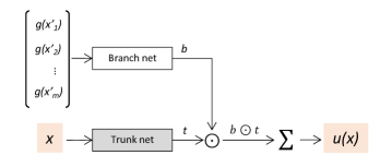
(a) DeepONet

(b) Deep Compositional Operator Network

Figure 1: The connection between our model architecture and DeepONet is shown. The architecture on the left is DeepONet and the one on the right is our proposed model. Comparing two model architectures, we can observe that our model is a compositional version of the DeepONet.

Without loss of generality, let us consider a PDE operator mapping from boundary conditions to the PDE solution, denoted by $\mathcal{M}:g(\bm{x}^{\prime})\rightarrow u(\bm{x})$. In DCON, similarly to DeepONet, the boundary conditions is encoded using a finite number of sampled boundary conditions $[\bm{x}^{\prime}_{1},\bm{x}^{\prime}_{2},...,\bm{x}^{\prime}_{m}]$, and the corresponding function values $[g(\bm{x}^{\prime}_{1}),g(\bm{x}^{\prime}_{2}),...,g(\bm{x}^{\prime}_{m})]$. The architecture of DCON consists of a "branch network" and a "solution network". The branch network maps the given boundary conditions on each of the available $m$ boundary locations to a higher dimensional space, $\mathcal{S}_{\text{param}}$, using a multi-layer perceptron. Then, a Max-pooling layer is applied to this high-dimensional representation to capture, in each dimension of $\mathcal{S}_{\text{param}}$, the most important feature across the $m$ locations on the boundary. The final output of the branch network is a global parameter embedding $\bm{b}$ in the high-dimensional space $\mathcal{S}_{\text{param}}$, whose dimension is independent of the number of boundary points, $m$. This setup relaxes the requirement for all training and test data to include the same number of boundary locations, $m$.

The inputs to the solution network are the coordinates of a collocation point, denoted by $\bm{x}$, and the parameter embedding, $\bm{b}$, based on which the solution at the collocation points $u(\bm{x})$ is calculated. As shown in equation 8, the functional mapping $\mathcal{M}$ is approximated with a number of operator layers $H$ formulated as following:

$$v^{l+1}=H(v^{l}):=\bm{b}\odot N(v^{l}),$$ (9)

where $v^{l}$ represents the output of $l$-th operator layer. In our proposed model, we simply use a linear layer with a nonlinear activation function as the mapping $N$. Hence, the PDE operator can be approximated by our proposed model using the following equation:

$$\mathcal{M}\approx\text{sum}\{\bm{b}\odot...(\bm{b}\odot(W^{2}_{L}\ \sigma(\bm{b}\odot(W^{1}_{L}\ \sigma(W_{\bm{t}}\bm{x}+B_{\bm{t}})+B^{1}_{L}))+B^{2}_{L}))\},$$ (10)

where $\sigma$ represents the nonlinear activation function, $W_{\bm{t}}\in R^{q\times d},B_{\bm{t}}\in R^{q}$ are trainable parameters of the mapping $\bm{t}$, and $W^{j}_{L}\in R^{q\times q},B^{j}_{L}\in R^{q}$ are trainable parameters of the $j$-th mapping $N$. These parameters of the model are optimized by minimizing the physics-informed training loss as shown in equation 2. More details about the proposed model architecture are shown in Figure 2. It should be noted that the proposed DCON architecture can also be used in a data-driven approach, where its parameters are estimated in a supervised learning process, as will be discussed in Section 4.3.

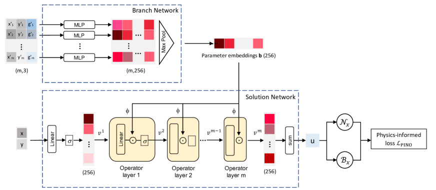
Figure 2: The architecture of the physics-informed Deep Compositional Operator Network is shown. The grey blocks represent the coordinates and the blue blocks represent the function values. The red blocks represent the hidden embeddings. The value of $b^{\prime}_{i}$ is the boundary condition value evaluated on $(x^{\prime}_{i},y^{\prime}_{i})$. The value of $u$ is the solution value evaluated on $(x,y)$. It should be noted that no activation function is included in the last operator layer.

4 Numerical results

In this section, we numerically evaluate the accuracy of the proposed model for solving parametric differential equations. We compare our models with data-driven DeepONet Lu et al. (2021) and physics-informed DeepONet Wang et al. (2021). We use these default settings unless mentioned otherwise; We use the hyperbolic tangent function (Tanh) Lau and Lim (2018) as our activation function to ensure the smoothness in high-order derivatives. For the architecture of DeepONet, we use three hidden layers of width 512. For our model architecture, we use three operator layers of width 512. Adam is the default optimizer with the following default hyper-parameters: $\beta_{1}$ = 0.9 and $\beta_{2}$ = 0.999 Kingma and Ba (2014). Each model is trained on 70% of the sampled PDE parameters and validated on 10% of the sampled PDE parameters. Well-trained models predict the PDE solution for the remaining 20% of the sampled PDE parameters. Two hyper-parameters used in model training: (1) the learning rate, with the possible values of learning rate are 0.001, 0.0005, 0.0002, and 0.0001; and (2) the coordinate sampling size ratio in each epoch. This ratio determines the number of collocation points in each epoch as a function of the number of sampled PDE parameters. The possible values for this ratio are 0.3, 0.2, 0.1, and 0.05. We implement grid search Bergstra and Bengio (2012) to calculate the best hyper-parameters, for which report the corresponding model performances are reported. Model training is performed on an NVIDIA P100 GPU using a batch size of 20. We collect the parameters of PDEs by Monte Carlo Simulation Harrison (2010) of stochastic processes Parzen (1999) and derive the solution of PDEs based on the Finite Element Method using Matlab Matlab (2012).

4.1 Experiment Setups

4.1.1 A Darcy flow problem

Let us consider a two-dimensional Darcy flow problem in a pentagram-shaped domain with a hole inside, which is a benchmark problem studied by a data-driven neural operator used in Lu et al. (2022). The steady state solution of the system is described by the following equation:

$$-\nabla(k(x,y)\nabla p(x,y)) =f(x,y),\quad(x,y)\in\Omega,$$ (11)

where $p(x,y)$ is the pressure, $k(x,y)$ is the permeability field, $f(x,y)$ is the source term, and $g(x,y)$ is the prescribed pressure on the domain boundaries. Using the same setting of Lu et al. (2022), we consider $k(x,y)=1$ and $f(x,y)=10$. The boundary consists of two parts, i.e. $\partial\Omega=\partial\Omega_{1}\cup\partial\Omega_{2}$. First, on the perimeter of the hole, denoted by $\partial\Omega_{1}$, the pressure is set to be zero. Second, on the outer edges of the pentagram, denoted by $\partial\Omega_{2}$, we impose a nonzero boundary condition function $g$. Hence, the boundary conditions of the problem is formulated as:

$$p(x,y) =0, (x,y)\in\partial\Omega_{1},$$ (12)

$$p(x,y) =g(x,y), (x,y)\in\partial\Omega_{2}.$$

In this example, we consider the pressure on $\partial\Omega_{2}$ to follow a zero mean Gaussian process with a covariance kernel that is only dependent on the horizontal distance, i.e.,

$$g(x,y) \sim\mathcal{GP}(0,K(x,x^{\prime})),$$ (13)

$$K(x,x^{\prime}) =\exp\left[-\frac{(x-x^{\prime})^{2}}{2l^{2}}\right].$$

We employ this Gaussian process model of Eq. 13 with $l=1$ to generate $N=1000$ different imposed pressure functions on $\partial\Omega_{2}$. Then given these sampled functions, $\{g_{i}\}_{i=1}^{N}$ we solve the PDE using Finite Element Method (FEM) Li and Chen (2019). In order to demonstrate the resol-independence feature of our model, for different sampled boundary functions, we consider different mesh sizes in the domain. Specifically, for the $i$-th realization, with the boundary condition function $g_{i}$, let $M_{1,i}$ and $M_{2,i}$ be the number of sampled locations on $\partial\Omega_{1}$ and $\partial\Omega_{2}$, respectively, and $\bm{X}_{\text{BC}_{1},i}$ and $\bm{X}_{\text{BC}_{2},i}$ are the corresponding sets of coordinates at those sampled locations, i.e.

$$\bm{X}_{\text{BC}_{1},i}=\{(x_{j}^{1,i},y_{j}^{1,i})\}_{j=1}^{M^{1,i}},$$ (14)

$$\bm{X}_{\text{BC}_{2},i}=\{(x_{j}^{2,i},y_{j}^{2,i})\}_{j=1}^{M^{2,i}},$$

Specifically, we choose $M_{1,i}$ and $M^{2,i}$ to be random numbers drawn from $[30,80]$ and from $[100,300]$, respectively. Therefore, all the boundary information for a single data is collected in $\bm{G}^{i}$ as:

$$\bm{G}_{i}=\{\bm{X}_{\text{BC}_{2},i},g_{i}(\bm{X}_{\text{BC}_{2},i})\},$$ (15)

where $g_{i}(\bm{X}_{\text{BC}_{2},i})$ is the boundary values evaluated at the coordinates $\bm{X}_{\text{BC}_{2},i}$. Figure  3 shows visualizations of a few sampled boundary conditions together on the finest and coarsest meshes used in this study.

Figure 3: The boundary conditions of our Darcy flow experiment setting, and the coarsest and finest meshes used as discretizations to solve the PDE are shown. The samples of Gaussian processes as the boundary conditions $g(\bm{x})$ are also shown above the meshes. The dots on the curve are considered as the representation of the boundary condition values.

Given this setup, we seek to learn the nonlinear mapping $\mathcal{M}_{\text{Darcy}}$ that transforms a given boundary conditions $g(x,y)$ on $\partial\Omega_{2}$ to the pressure field $p(x,y)$ in the entire domain, i.e.,

$$\mathcal{M}_{\text{Darcy}}:g(x,y)\rightarrow p(x,y).$$ (16)

Specifically, for a 2D problem, the neural operator $p_{\theta}(x,y,\bm{G})$ is trained using the loss function

$$\mathcal{L}(\theta)=\mathcal{L}_{\text{PDE}}(\theta)+\alpha_{1}\mathcal{L}_{\text{BC}_{1}}(\theta)+\alpha_{2}\mathcal{L}_{\text{BC}_{2}}(\theta),$$ (17)

where $\alpha_{1}$, $\alpha_{2}$ are the weighing hyperparameters, set to be $\alpha_{1}=\alpha_{2}=500$ to ensure similar orders of magnitude. $\mathcal{L}_{\text{PDE}}(\theta)$ and $\mathcal{L}_{\text{BC}}(\theta)$ are the PDE residual and the BC loss function, given by

$$\mathcal{L}_{\text{PDE}}(\theta) =\frac{1}{N}\sum_{i=1}^{N}\left[\frac{\partial^{2}p_{\theta}(x,y,\bm{G}_{i})}{\partial x^{2}}+\frac{\partial^{2}p_{\theta}(x,y,\bm{G}_{i})}{\partial y^{2}}+10\right]^{2}, (x,y)\in\Omega,$$ (18)

$$\mathcal{L}_{\text{BC}_{1}}(\theta) =\frac{1}{N}\sum_{i=1}^{N}\left\{\frac{1}{M_{1,i}}\sum_{j=1}^{M_{1,i}}\left[p_{\theta}(x^{i}_{j},y^{i}_{j},\bm{G}_{i})-0\right]^{2}\right\}, (x^{i}_{j},y^{i}_{j})\in\bm{X}_{\text{BC}_{1},i},$$

$$\mathcal{L}_{\text{BC}_{2}}(\theta) =\frac{1}{N}\sum_{i=1}^{N}\left\{\frac{1}{M_{2,i}}\sum_{j=1}^{M_{2,i}}\left[p_{\theta}(x^{i}_{j},y^{i}_{j},\bm{G}_{i})-g_{i}(x^{i}_{j},y^{i}_{j})\right]^{2}\right\}, (x^{i}_{j},y^{i}_{j})\in\bm{X}_{\text{BC}_{2},i}.$$

4.1.2 A 2D plate problem

In this example, we consider more complex problems where a nonlinear mapping between multiple parameter functions and multiple response functions is to be learned. In particular, let us consider a two-dimensional rectangular elastic plate with a central hole (similar to the example in Li et al. (2021a)). The steady state solution for the plate displacements is governed by the following system of partial differential equations

$$\frac{E}{1-\mu^{2}}\left[\frac{\partial^{2}u(x,y)}{\partial x^{2}}+\frac{(1-\mu)}{2}\frac{\partial^{2}u(x,y)}{\partial y^{2}}+\frac{(1+\mu)}{2}\frac{\partial^{2}v(x,y)}{\partial x\partial y}\right] =0,\quad(x,y)\in\Omega,$$ (19)

$$\frac{E}{1-\mu^{2}}\left[\frac{\partial^{2}v(x,y)}{\partial y^{2}}+\frac{(1-\mu)}{2}\frac{\partial^{2}v(x,y)}{\partial x^{2}}+\frac{(1+\mu)}{2}\frac{\partial^{2}u(x,y)}{\partial x\partial y}\right] =0,\quad(x,y)\in\Omega,$$

where $u$ and $v$ are the plate displacements in $x$ and $y$ directions, respectively, $E$ is the Young’s Modules, and $\mu$ is the Poisson’s Ratio.

The plate is 20 mm × 20 mm, and the hole has a diameter of 5 mm. We impose different boundary conditions on the different edges of the plate. The edge surrounding the central hole is subjected to a fixed boundary condition and there are imposed displacements on the left and right sides. The top and bottom sides are assigned free boundary conditions. The complete boundary conditions are shown in Figure  4, and are given by

$$u(x,y)=0,\quad v(x,y)=0, (x,y)\in\partial\Omega_{\text{H}},$$ (20)

$$u(x,y)=u_{l}(x,y),\quad v(x,y)=v_{l}(x,y) (x,y)\in\partial\Omega_{\text{L}},$$

$$u(x,y)=u_{R}(x,y),\quad v(x,y)=v_{R}(x,y) (x,y)\in\partial\Omega_{\text{R}},$$

$$\frac{\partial v(x,y)}{\partial y}=0,\quad\frac{1}{2}\left[\frac{\partial u(x,y)}{\partial y}+\frac{\partial v(x,y)}{\partial x}\right]=0, (x,y)\in\partial\Omega_{\text{TB}}.$$

where the prescribed displacement functions $u_{l},v_{l},u_{R},v_{R}$ are the inputs to the operator. Similar to previous example, these functions are considered to follow a Gaussian Process model. The covariance kernel is assumed to be dependent only on the vertical distance, i.e.,

$$u_{l},v_{l},u_{R},v_{R} \sim\mathcal{GP}(1,K(y,y^{\prime})),$$ (21)

$$K(y,y^{\prime}) =\exp\left[-\frac{(y-y^{\prime})^{2}}{2l^{2}}\right].$$

We used $l=5$, and similarly to previous example, we draw $N=1000$ realizations of these functions, and obtain FE solutions using meshes with different sizes. Figure 4 shows the finest and coarsest meshes with a few samples of imposed displacement functions. The boundary condition information on the left and right sides for the $i$-th realization is collected into the following two vectors, model as follows:

$$\bm{X}_{\text{BC}_{\text{H}},i}=\{(x_{j}^{1,i},y_{j}^{1,i})\}_{j=1}^{M_{1,i}},$$ (22)

$$\bm{X}_{\text{BC}_{\text{L}},i}=\{(x_{j}^{2,i},y_{j}^{2,i})\}_{j=1}^{M_{2,i}},$$

$$\bm{X}_{\text{BC}_{\text{R}},i}=\{(x_{j}^{3,i},y_{j}^{3,i})\}_{j=1}^{M_{3,i}},$$

$$\bm{X}_{\text{BC}_{\text{TB}},i}=\{(x_{j}^{4,i},y_{j}^{4,i})\}_{j=1}^{M_{4,i}},$$

where $\bm{X}_{\text{BC}_{\text{H}},i}$, $\bm{X}_{\text{BC}_{\text{L}},i}$, $\bm{X}_{\text{BC}_{\text{R}},i}$, $\bm{X}_{\text{BC}_{\text{TB}},i}$ are the sets of boundary coordinates of $\partial\Omega_{\text{H}}$, $\partial\Omega_{\text{L}}$, $\partial\Omega_{\text{R}}$, $\partial\Omega_{\text{TB}}$, respectively. The prescribed displacement information as inputs to the model $\bm{G}_{L,i}$ and $\bm{G}_{R,i}$ are formulated as:

$$\bm{G}_{L,i} =\{\bm{X}_{\text{BC}_{L},i},u_{L,i}(\bm{X}_{\text{BC}_{L},i}),v_{L,i}(\bm{X}_{\text{BC}_{L},i})\},$$ (23)

$$\bm{G}_{R,i} =\{\bm{X}_{\text{BC}_{R},i},u_{R,i}(\bm{X}_{\text{BC}_{R},i}),v_{R,i}(\bm{X}_{\text{BC}_{R},i})\}.$$

Given this setup, we seek to learn the nonlinear mapping $\mathcal{M}_{\text{Plate}}$ that transforms a given prescribed displacement functions $u_{L}(x,y),v_{L}(x,y),u_{R}(x,y),v_{R}(x,y)$ on $\partial\Omega_{\text{L}}$ and $\partial\Omega_{\text{R}}$ to the displacement field $u(x,y)$ and $v(x,y)$ in the entire domain, i.e.,

$$\mathcal{M}_{\text{Plate}}:[u_{L}(x,y),v_{L}(x,y),u_{R}(x,y),v_{R}(x,y)]\rightarrow[u(x,y),v(x,y)].$$ (24)

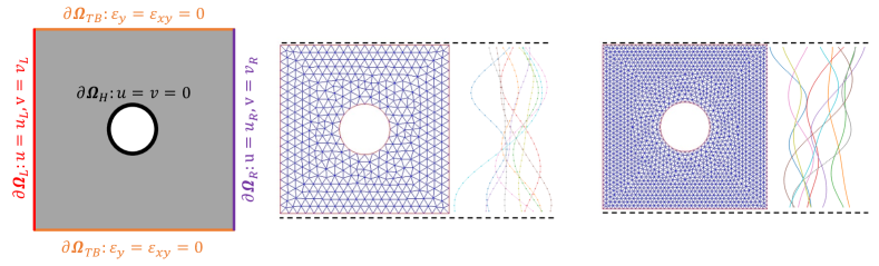
Figure 4: The boundary conditions of 2D plate experiment, and the coarsest and finest meshes used as discretizations to solve the PDE are shown. The samples of Gaussian processes as the prescribed displacement on leftmost edges and rightmost edges are also shown. The dots on the curve are considered as the representation of the prescribed displacements.

Based on our boundary condition settings, the training loss function $\mathcal{L}(\theta)$ for training the neural operators $u_{\theta}(x,y,\bm{G}_{L},\bm{G}_{R})$ and $v_{\theta}(x,y,\bm{G}_{L},\bm{G}_{R})$ is formulated as:

$$\mathcal{L}(\theta)=\alpha_{0}\mathcal{L}_{\text{PDE}}(\theta)+\alpha_{2}\mathcal{L}_{\text{BC}_{\text{H}}}(\theta)+\alpha_{2}\mathcal{L}_{\text{BC}_{\text{L}}}(\theta)+\alpha_{3}\mathcal{L}_{\text{BC}_{\text{R}}}(\theta)+\alpha_{4}\mathcal{L}_{\text{BC}_{\text{TB}}}(\theta),$$ (25)

where $\alpha_{0}$, $\alpha_{1}$, $\alpha_{2}$, $\alpha_{3}$, $\alpha_{4}$ are the trade-off coefficient, set to be $\alpha_{0}=0.00001,\alpha_{1}=\alpha_{2}=\alpha_{3}=\alpha_{4}=1$ to ensure similar orders of magnitude, $\mathcal{L}_{\text{PDE}}(\theta)$ is the PDE residual given by

$$\mathcal{L}_{\text{PDE}}(\theta)=\frac{1}{N}\sum_{i=1}^{N} \left\{\frac{E}{1-\mu^{2}}\left(\frac{\partial^{2}u_{\theta}(x,y,\bm{G}_{L,i},\bm{G}_{R,i})}{\partial x^{2}}+\frac{\partial^{2}v_{\theta}(x,y,\bm{G}_{L,i},\bm{G}_{R,i})}{\partial y^{2}}\right)+\right.$$ (26)

$$\left.\frac{E}{2(1+\mu)}\left(\frac{\partial^{2}u_{\theta}(x,y,\bm{G}_{L,i},\bm{G}_{R,i})}{\partial y^{2}}+\frac{\partial^{2}v_{\theta}(x,y,\bm{G}_{L,i},\bm{G}_{R,i})}{\partial x^{2}}\right)+\right.$$

$$\left.\frac{E}{2(1-\mu)}\left(\frac{\partial^{2}v_{\theta}(x,y,\bm{G}_{L,i},\bm{G}_{R,i})}{\partial x\partial y}+\frac{\partial^{2}u_{\theta}(x,y,\bm{G}_{L,i},\bm{G}_{R,i})}{\partial x\partial y}\right)\right\},\quad(x,y)\in\Omega,$$

and $\mathcal{L}_{\text{BC}_{\text{H}}}(\theta)$, $\mathcal{L}_{\text{BC}_{\text{L}}}(\theta)$, $\mathcal{L}_{\text{BC}_{\text{R}}}(\theta)$, $\mathcal{L}_{\text{BC}_{\text{TB}}}(\theta)$ are the BC losses, given by

$$\mathcal{L}_{\text{BC}_{\text{H}}}(\theta)=\frac{1}{N}\sum_{i=1}^{N} \left\{\frac{1}{M_{1,i}}\sum_{j=1}^{M_{1,i}}\left[u_{\theta}(x_{j}^{i},y_{j}^{i},\bm{G}_{L,i},\bm{G}_{R,i})-0\right]^{2}+\left[v_{\theta}(x_{j}^{i},y_{j}^{i},\bm{G}_{L,i},\bm{G}_{R,i})-0\right]^{2}\right\},$$ (27)

$$\qquad\qquad\qquad\qquad\qquad\qquad\qquad\qquad\qquad\qquad\qquad\qquad\qquad\qquad\qquad\qquad{(x_{j}^{i},y_{j}^{i})\in\bm{X}_{\text{BC}_{\text{H}},i},}$$

$$\mathcal{L}_{\text{BC}_{\text{L}}}(\theta)=\frac{1}{N}\sum_{i=1}^{N} \left\{\frac{1}{M_{2,i}}\sum_{j=1}^{M_{2,i}}\left[u_{\theta}(x_{j}^{i},y_{j}^{i},\bm{G}_{L,i},\bm{G}_{R,i})-u_{L,i}(x_{j}^{i},y_{j}^{i})\right]^{2}+\left[v_{\theta}(x_{j}^{i},y_{j}^{i},\bm{G}_{L,i},\bm{G}_{R,i})-v_{L,i}(x_{j}^{i},y_{j}^{i})\right]^{2}\right\},$$

$$\qquad\qquad\qquad\qquad\qquad\qquad\qquad\qquad\qquad\qquad\qquad\qquad\qquad\qquad\qquad\qquad{(x_{j}^{i},y_{j}^{i})\in\bm{X}_{\text{BC}_{\text{L}},i},}$$

$$\mathcal{L}_{\text{BC}_{\text{R}}}(\theta)=\frac{1}{N}\sum_{i=1}^{N} \left\{\frac{1}{M_{3,i}}\sum_{j=1}^{M_{3,i}}\left[u_{\theta}(x_{j}^{i},y_{j}^{i},\bm{G}_{L,i},\bm{G}_{R,i})-u_{R,i}(x_{j}^{i},y_{j}^{i})\right]^{2}+\left[v_{\theta}(x_{j}^{i},y_{j}^{i},\bm{G}_{L,i},\bm{G}_{R,i})-v_{R,i}(x_{j}^{i},y_{j}^{i})\right]^{2}\right\},$$

$$\qquad\qquad\qquad\qquad\qquad\qquad\qquad\qquad\qquad\qquad\qquad\qquad\qquad\qquad\qquad\qquad{(x_{j}^{i},y_{j}^{i})\in\bm{X}_{\text{BC}_{\text{R}},i},}$$

$$\mathcal{L}_{\text{BC}_{\text{TB}}}(\theta)=\frac{1}{N}\sum_{i=1}^{N} \left\{\frac{1}{M_{4,i}}\sum_{j=1}^{M_{4,i}}\left[\frac{\partial v_{\theta}(x_{j}^{i},y_{j}^{i},\bm{G}_{L,i},\bm{G}_{R,i})}{\partial y_{j}^{i}}-0\right]^{2}+\right.$$

$$\left.\left[\frac{1}{2}\left(\frac{\partial u_{\theta}(x_{j}^{i},y_{j}^{i},\bm{G}_{L,i},\bm{G}_{R,i})}{\partial y_{j}^{i}}+\frac{\partial v_{\theta}(x_{j}^{i},y_{j}^{i},\bm{G}_{L,i},\bm{G}_{R,i})}{\partial x_{j}^{i}}\right)-0\right]^{2}\right\},$$

$$\qquad\qquad\qquad\qquad\qquad\qquad\qquad\qquad\qquad\qquad\qquad\qquad\qquad\qquad\qquad\qquad{(x_{j}^{i},y_{j}^{i})\in\bm{X}_{\text{BC}_{\text{TB}},i}.}$$

4.2 Main results

For each problem, we conduct two experiments. First, in order to compare our method with PI-DeepONet, which can only handle data with the same mesh size, we consider a fixed mesh size, taken to be small, for all the training and test cases. In the second experiment, we relax this constraint and generate training and test data each with a variable mesh size. The comparison between our proposed methods and the PI-DeepONet is summarized in Table  LABEL:fig.PI_com. We use the relative $L_{2}$ error to evaluate the accuracy of models. We report the average error calculated across the entire test dataset, along with the standard deviation of the relative errors, to demonstrate the model stability. Our proposed model showed satisfactory mean performance in both the Darcy flow problem and the 2D plate problem. Compared with physics-informed DeepONet, our model achieved 64.8% accuracy improvement for the Darcy flow problem and 68.1% accuracy improvement for the 2D plate problem. Based on the standard deviation of relative errors, our model also shows higher stability.

In the second experiment, when variable mesh sizes are used, compared to the fixed mesh size experiment, we note that PI-DCON shows reduction in accuracy for both the Darcy flow and the 2D plate problems. These results are reasonable, especially considering the 2D plate problem is inherently more complex. Despite these challenges, our model is able to maintain acceptable levels of accuracy, with mean relative errors below 3.5% for both problems.

Table 2: Accuracy comparison between PI-DCON and PI-DeepONet.

	Mean of relative error		Standard deviation of relative error
Experiment	PI-DeepONet	PI-DCON	PI-DeepONet	PI-DCON
Darcy flow (fixed mesh size)	7.10%	2.50%	4.00%	1.11%
2D plate (fixed mesh size)	5.58%	1.77%	1.14%	0.42%
Darcy flow (variable mesh size)	-	3.42%	-	1.43%
2D plate (variable mesh size)	-	2.98%	-	0.92%

In order to better visualize our model performances, we present histograms of the estimated relative error across the entire test dataset in Figures 5 and 6. Figure 5 demonstrates that, for most instances, our model predicts the PDE solutions with a relative error under 4%, whereas the relative error for most of the predictions of PI-DeepONet falls within the 4% to 10% range. In Figure 6, we also show that our model can handle varying mesh size with similar prediction accuracy as the fixed mesh size, achieving relative error under 6% for predictions of most cases. Figure 6 further illustrates that our model maintains comparable prediction accuracy across different mesh sizes. For the majority of predictions, it manages to keep the relative error below 6%.

Additionally, it’s noted that each model occasionally produces significantly poor predictions for certain test dataset samples. These instances are considered as outliers within the sample distribution. This phenomenon suggests that all the trained models demonstrate a deficiency in sustaining acceptable performance on samples that fall outside of the distribution, which will be an interesting problem to be investigated in the future works.

(a) Darcy flow

(b) 2D plate

Figure 5: Comparison between PI-DCON and PI-DeepONet on the Darcy flow and 2D plate problems, with the fixed mesh size.

(a) Darcy flow

(b) 2D plate

Figure 6: Comparison of PI-DCON for fixed mesh size versus variable mesh size, on the Darcy flow and 2D plate problems.

We also investigate the average model performance over the whole domain in the geometry in Table  3. Overall, our model achieved better performance than PI-DeepONet. Also, We observe that the models have difficulties in predicting the PDE solutions on the boundaries of varying boundary conditions. This indicates a larger trade-off coefficient for the hard constraints of the varying boundary conditions may be needed. However, setting this coefficient too high could impede the minimization of PDE residuals, indicating the need for future research to find an optimal balance for the trade-off coefficient.

When examining errors along the boundaries, we particularly notice that larger errors tend to appear at the boundary’s sharp angles, such as the concave angles in the pentagram and the corner angles of the 2D plate. This discrepancy could stem from imprecise gradient computations at these points, highlighting the importance of paying extra attention to the sharp angles in the geometry during physics-informed training processes.

Table 3: Comparison between Mean Absolute Errors shown over the domain

	PI-DeepONet (fixed mesh size)	PI-DCON (fixed mesh size)	PI-DCON (variable mesh size)
Darcy flow
2D plate

To further illustrate the comparative performance of our model, Tables  4 show predicted and ground truth solutions for PI-DeepONet and PI-DCON. For each problem, four of the test cases are shown. In particular, the test cases (i.e. realizations of boundary conditions) that cause the best and worst performances of PI-DeepONet and PI-DCON. It can be seen that our model shows higher accuracy, and maintains remarkable accuracy even in the most challenging (worst-case) scenario. Furthermore, the relatively small performance gap between the worst and best cases also highlights the robustness of our model. Furthermore, as can be seen in Table 5, PI-DCON can also produce acceptable predictions when training and test cases are created with variable mesh sizes.

Table 4: Comparison between the performance of PI-DCON and PI-DeepONet. Out of all realizations of boundary conditions, the ones that causes best and worst performances of each model are shown.

		Ground Truth	PI-DeepONet		PI-DCON
			Prediction	Absolute Error	Prediction	Absolute Error
Darcy flow	PI-DeepONet Best case
	PI-DCON Best case
	PI-DeepONet Worst case
	PI-DCON Worst case
2D Plate	PI-DeepONet Best case
	PI-DCON Best case
	PI-DeepONet Worst case
	PI-DCON Worst case

Table 5: Performance of PI-DCON trained with variable mesh sizes. The best and worst prediction among various realizations of boundary conditions are shown.

		Ground Truth	Prediction	Absolute Error
Darcy flow	Best case
	Worst case
2D plate	Best case
	Worst case

4.3 Comparison with data-driven neural operators

One of the main features of PI-DCON is that it is a data-free approach. It doesn’t require FE simulation runs as a training set. In this section, we seek to investigate its efficiency and accuracy in comparison with data-driven (supervised) training approaches. In doing so, we consider the data-driven DeepONet and also create a data-driven variant of our proposed DCON architecture for comparison. We first compare the performance of data-driven DCON with that of data-driven DeepONet in Table LABEL:table.data_driven_com. We observe that the DCON model achieved 44% accuracy improvement for the Darcy flow problem and 58% accuracy improvement for the 2D plate problem. Also, when we compare our model’s performance on data with variable mesh sizes to those with a fixed mesh size, we do not observe a significant drop in the prediction accuracy, which is comparable to the drop observed in PI-DCON.

Table 6: Accuracy comparison between data-driven DCON and data-driven DeepONet.

Dataset	Mean of relative error		Standard deviation of relative error
	Data-driven DeepONet	Data-driven DCON	Data-driven DeepONet	Data-driven DCON
Darcy flow (fixed mesh size)	3.74%	2.09%	0.97%	0.51%
2D plate (fixed mesh size)	3.78%	1.57%	1.01%	0.37%
Darcy flow (variable mesh size)	-	2.22%	-	0.59%
2D plate (variable mesh size)	-	1.78%	-	0.35%

In order to demonstrate the advantage of physics-informed (data-free) training of DCON, in Figure 7 we show the required timea need for building models at different accuracy levels. The horizontal (dashed) line represents the required CPU time for generating training datasets for data-driven training of neural operators. In both darcy flow and 2d plate problems, the lowest error rate achieved by PI-DCON is smaller than that of data-driven DeepONet but greater than that of data-driven DCON. This result suggests that neural operators trained in a data-driven fashion tend to outperform those trained using physics-informed approaches when the same model architecture is used. However, it can be seen that PI-DCON convergence is superior compared to data-driven DeepONet. This shows the enhanced architectural design in DCON improves alows for faster convergence compared to the conventional DeepONet.

Moreover, PI-DCON demonstrates greater training efficiency. This is when we compare the total time needed to train a model, including the time to obtain training data in the data-driven approaches. It was observed that PI-DCON required only 55% of the total time needed by data-driven DCON in the Darcy flow problem and 31% in the 2D plate problem. This efficiency gain suggests that adopting a physics-informed training approach can lead to significant computational time savings, especially for more complex problems.

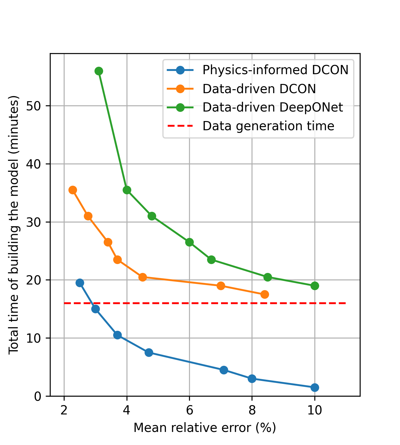
(a) Darcy flow problem

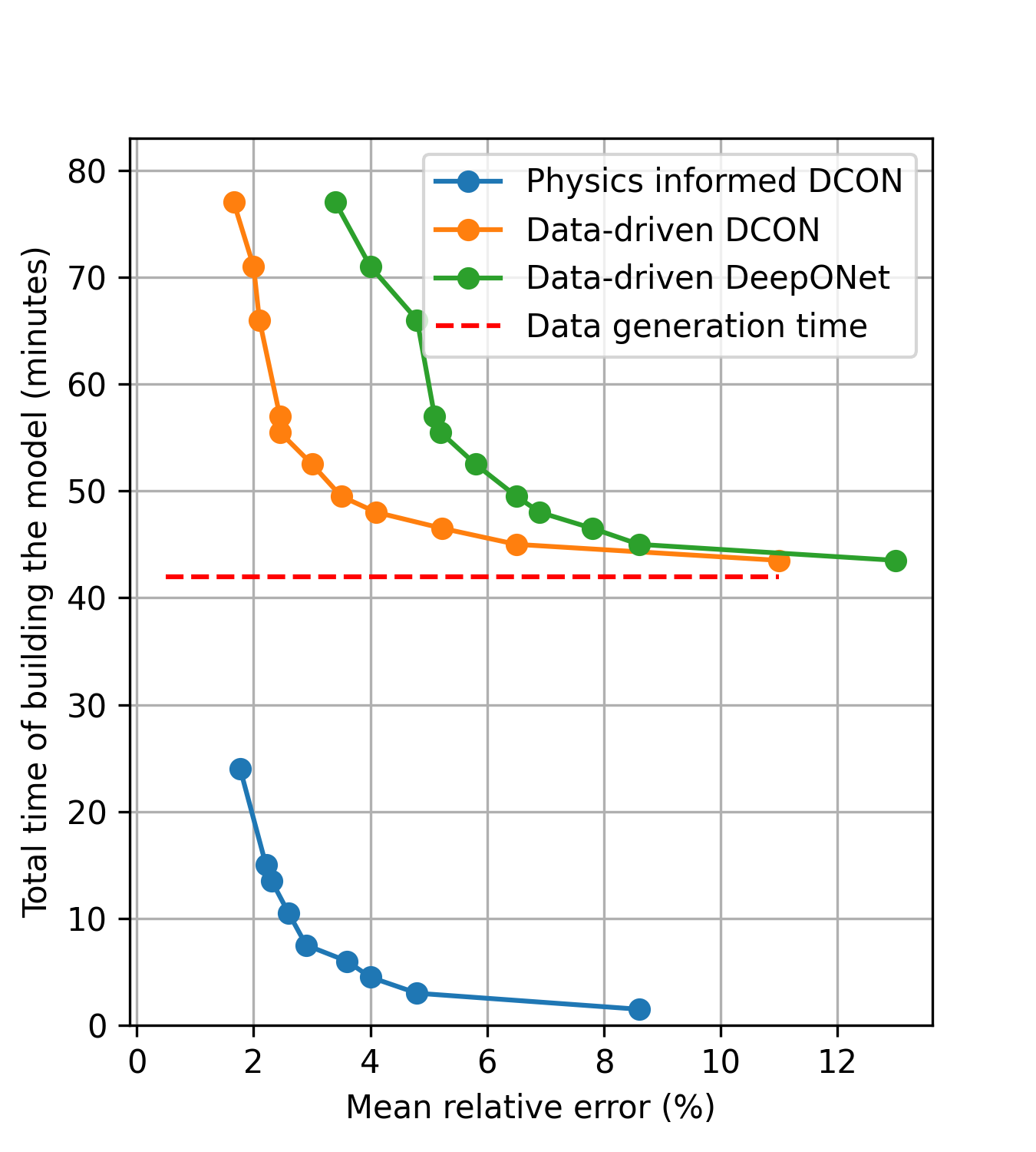
(b) 2D plate problem

Figure 7: Comparison between the total time needed to train different neural operators. For data-driven method, this time also includes the time needed to generate the training (FE simulation) data.

4.4 Ablation studies

In this section, we conduct ablation studies on the proposed PI-DCON model, with a particular emphasis on how the number of operator layers affects the accuracy. To this end, we train PI-DCON models with varying numbers of operator layers (specifically, 1, 2, 3, and 4) for 500 epochs, and report the prediction accuracies in Table  LABEL:table.ablation_num_layer. We observe that an increase in the number of operator layers leads to improved accuracy. However, the marginal improvement in prediction accuracy diminishes with each additional layer. For example, increasing the layer count from 1 to 2 yields an average accuracy improvement of 3.79%, whereas the increment from 3 to 4 results in a mere 0.45% improvement.

Table 7: Mean of relative error of different model sizes.

	Number of operator layers
	1	2	3	4	5	6
Darcy flow (fixed mesh size)	10.10%	4.20%	2.50 %	2.15%	2.06%	2.03%
2D plate (fixed mesh size)	5.92%	2.57%	1.77%	1.56%	1.43%	1.38%
Darcy flow (variable mesh size)	12.58%	5.01%	3.42%	2.83%	2.66%	2.59%
2D plate (variable mesh size)	7.83%	4.52%	2.98%	2.34%	2.16%	2.07%

5 Conclusion

In this study, we presented an enhanced architecture for physics-informed training of neural operators. We introduced PI-DCON based on the inspiration from the Universal Approximation Theorem underlying the development of DeepONet. Our results indicate that PI-DCON achieves superior accuracy and generalization capabilities compared to PI-DeepONet. Furthermore, the comparison between our model with data-driven neural operators highlights the advantages of developing neural operators using a physics-informed training approach.

Despite these advancements, our approach has its limitations. Primarily, the current model architecture is designed to generalize across various meshes of different size but does not extend this generalization to differing domain shapes. Furthermore, our evaluation focuses solely on the model’s capability in computing steady-state solutions. Further research is needed to extend PI-DCON to also incorporate dynamic responses, thereby enabling it to tackle time-dependent PDEs. Additionally, while our model currently relies on the basic multi-layer perceptron structure, incorporating more sophisticated architectures, such as Attention Mechanisms Vaswani et al. (2017), may further enhance its performance.

References

- Baddoo et al. [2023] Peter J Baddoo, Benjamin Herrmann, Beverley J McKeon, J Nathan Kutz, and Steven L Brunton. Physics-informed dynamic mode decomposition. Proceedings of the Royal Society A, 479(2271):20220576, 2023.
- Beltrán-Pulido et al. [2022] Andrés Beltrán-Pulido, Ilias Bilionis, and Dionysios Aliprantis. Physics-informed neural networks for solving parametric magnetostatic problems. IEEE Transactions on Energy Conversion, 37(4):2678–2689, 2022.
- Bergstra and Bengio [2012] James Bergstra and Yoshua Bengio. Random search for hyper-parameter optimization. Journal of machine learning research, 13(2), 2012.
- Chen et al. [2021] Zhao Chen, Yang Liu, and Hao Sun. Physics-informed learning of governing equations from scarce data. Nature communications, 12(1):6136, 2021.
- Dhatt et al. [2012] Gouri Dhatt, Emmanuel Lefrançois, and Gilbert Touzot. Finite element method. John Wiley & Sons, 2012.
- Eschenauer and Olhoff [2001] Hans A Eschenauer and Niels Olhoff. Topology optimization of continuum structures: a review. Appl. Mech. Rev., 54(4):331–390, 2001.
- Goswami et al. [2022] Somdatta Goswami, Minglang Yin, Yue Yu, and George Em Karniadakis. A physics-informed variational deeponet for predicting crack path in quasi-brittle materials. Computer Methods in Applied Mechanics and Engineering, 391:114587, 2022.
- Goswami et al. [2023] Somdatta Goswami, Aniruddha Bora, Yue Yu, and George Em Karniadakis. Physics-informed deep neural operator networks. In Machine Learning in Modeling and Simulation: Methods and Applications, pages 219–254. Springer, 2023.
- Hansen et al. [2023] Derek Hansen, Danielle C Maddix, Shima Alizadeh, Gaurav Gupta, and Michael W Mahoney. Learning physical models that can respect conservation laws. In International Conference on Machine Learning, pages 12469–12510. PMLR, 2023.
- Harrison [2010] Robert L Harrison. Introduction to monte carlo simulation. In AIP conference proceedings, volume 1204, page 17. NIH Public Access, 2010.
- Henkes et al. [2022] Alexander Henkes, Henning Wessels, and Rolf Mahnken. Physics informed neural networks for continuum micromechanics. Computer Methods in Applied Mechanics and Engineering, 393:114790, 2022.
- Ketkar et al. [2021] Nikhil Ketkar, Jojo Moolayil, Nikhil Ketkar, and Jojo Moolayil. Automatic differentiation in deep learning. Deep Learning with Python: Learn Best Practices of Deep Learning Models with PyTorch, pages 133–145, 2021.
- Khoo et al. [2021] Yuehaw Khoo, Jianfeng Lu, and Lexing Ying. Solving parametric pde problems with artificial neural networks. European Journal of Applied Mathematics, 32(3):421–435, 2021.
- Kingma and Ba [2014] Diederik P. Kingma and Jimmy Ba. Adam: A method for stochastic optimization, 2014. URL https://arxiv.org/abs/1412.6980.
- Kovachki et al. [2021] Nikola Kovachki, Zongyi Li, Burigede Liu, Kamyar Azizzadenesheli, Kaushik Bhattacharya, Andrew Stuart, and Anima Anandkumar. Neural operator: Learning maps between function spaces. arXiv preprint arXiv:2108.08481, 2021.
- Lau and Lim [2018] Mian Mian Lau and King Hann Lim. Review of adaptive activation function in deep neural network. In 2018 IEEE-EMBS Conference on Biomedical Engineering and Sciences (IECBES), pages 686–690. IEEE, 2018.
- Li and Chen [2019] Jichun Li and Yi-Tung Chen. Computational partial differential equations using MATLAB®. Crc Press, 2019.
- Li et al. [2021a] Wei Li, Martin Z Bazant, and Juner Zhu. A physics-guided neural network framework for elastic plates: Comparison of governing equations-based and energy-based approaches. Computer Methods in Applied Mechanics and Engineering, 383:113933, 2021a.
- Li et al. [2020a] Zongyi Li, Nikola Kovachki, Kamyar Azizzadenesheli, Burigede Liu, Kaushik Bhattacharya, Andrew Stuart, and Anima Anandkumar. Fourier neural operator for parametric partial differential equations. arXiv preprint arXiv:2010.08895, 2020a.
- Li et al. [2020b] Zongyi Li, Nikola Kovachki, Kamyar Azizzadenesheli, Burigede Liu, Kaushik Bhattacharya, Andrew Stuart, and Anima Anandkumar. Neural operator: Graph kernel network for partial differential equations. arXiv preprint arXiv:2003.03485, 2020b.
- Li et al. [2021b] Zongyi Li, Hongkai Zheng, Nikola Kovachki, David Jin, Haoxuan Chen, Burigede Liu, Kamyar Azizzadenesheli, and Anima Anandkumar. Physics-informed neural operator for learning partial differential equations. arXiv preprint arXiv:2111.03794, 2021b.
- Li et al. [2023] Zongyi Li, Daniel Zhengyu Huang, Burigede Liu, and Anima Anandkumar. Fourier neural operator with learned deformations for pdes on general geometries. Journal of Machine Learning Research, 24(388):1–26, 2023.
- Lu et al. [2021] Lu Lu, Pengzhan Jin, Guofei Pang, Zhongqiang Zhang, and George Em Karniadakis. Learning nonlinear operators via deeponet based on the universal approximation theorem of operators. Nature Machine Intelligence, 3(3):218–229, March 2021. ISSN 2522-5839. doi:10.1038/s42256-021-00302-5. URL http://dx.doi.org/10.1038/s42256-021-00302-5.
- Lu et al. [2022] Lu Lu, Xuhui Meng, Shengze Cai, Zhiping Mao, Somdatta Goswami, Zhongqiang Zhang, and George Em Karniadakis. A comprehensive and fair comparison of two neural operators (with practical extensions) based on fair data. Computer Methods in Applied Mechanics and Engineering, 393:114778, 2022.
- Matlab [2012] Starting Matlab. Matlab. The MathWorks, Natick, MA, 2012.
- Mengaldo et al. [2022] Gianmarco Mengaldo, Federico Renda, Steven L Brunton, Moritz Bächer, Marcello Calisti, Christian Duriez, Gregory S Chirikjian, and Cecilia Laschi. A concise guide to modelling the physics of embodied intelligence in soft robotics. Nature Reviews Physics, 4(9):595–610, 2022.
- Moseley et al. [2023] Ben Moseley, Andrew Markham, and Tarje Nissen-Meyer. Finite basis physics-informed neural networks (fbpinns): a scalable domain decomposition approach for solving differential equations. Advances in Computational Mathematics, 49(4):62, 2023.
- Naderibeni et al. [2024] Mahdi Naderibeni, Marcel JT Reinders, Liang Wu, and David MJ Tax. Learning solutions of parametric navier-stokes with physics-informed neural networks. arXiv preprint arXiv:2402.03153, 2024.
- Navaneeth et al. [2024] N Navaneeth, Tapas Tripura, and Souvik Chakraborty. Physics informed wno. Computer Methods in Applied Mechanics and Engineering, 418:116546, 2024.
- Nguyen et al. [2023] Tung Nguyen, Johannes Brandstetter, Ashish Kapoor, Jayesh K Gupta, and Aditya Grover. Climax: A foundation model for weather and climate. arXiv preprint arXiv:2301.10343, 2023.
- O’Shea and Nash [2015] Keiron O’Shea and Ryan Nash. An introduction to convolutional neural networks. arXiv preprint arXiv:1511.08458, 2015.
- Parzen [1999] Emanuel Parzen. Stochastic processes. SIAM, 1999.
- Raissi et al. [2019] Maziar Raissi, Paris Perdikaris, and George E Karniadakis. Physics-informed neural networks: A deep learning framework for solving forward and inverse problems involving nonlinear partial differential equations. Journal of Computational physics, 378:686–707, 2019.
- Ren et al. [2022] Pu Ren, Chengping Rao, Yang Liu, Jian-Xun Wang, and Hao Sun. Phycrnet: Physics-informed convolutional-recurrent network for solving spatiotemporal pdes. Computer Methods in Applied Mechanics and Engineering, 389:114399, 2022.
- Tripura and Chakraborty [2022] Tapas Tripura and Souvik Chakraborty. Wavelet neural operator: a neural operator for parametric partial differential equations. arXiv preprint arXiv:2205.02191, 2022.
- Vaswani et al. [2017] Ashish Vaswani, Noam Shazeer, Niki Parmar, Jakob Uszkoreit, Llion Jones, Aidan N Gomez, Łukasz Kaiser, and Illia Polosukhin. Attention is all you need. Advances in neural information processing systems, 30, 2017.
- Wang et al. [2021] Sifan Wang, Hanwen Wang, and Paris Perdikaris. Learning the solution operator of parametric partial differential equations with physics-informed deeponets. Science advances, 7(40):eabi8605, 2021.
- Zhu et al. [2023] Qiming Zhu, Ze Zhao, and Jinhui Yan. Physics-informed machine learning for surrogate modeling of wind pressure and optimization of pressure sensor placement. Computational Mechanics, 71(3):481–491, 2023.