Effects of dynamical dielectric screening on the excitonic spectrum of monolayer semiconductors

Abstract

We present a new method to solve the dynamical Bethe-Salpeter Equation numerically. The method allows one to investigate the effects of dynamical dielectric screening on the spectral position of excitons in transition-metal dichalcogenide monolayers. The dynamics accounts for the response of optical phonons in the materials below and on top the monolayer to the electric field lines between the electron and hole of the exciton. The inclusion of this effect unravels the origin of a counterintuitive energy blueshift of the exciton resonance, observed recently in monolayer semiconductors that are supported on ionic crystals with large dielectric constants. A surprising result is that while energy renormalization of a free electron in the conduction band or a free hole in the valence band is controlled by the low-frequency dielectric constant, the bandgap energy introduces a phase between the photoexcited electron and hole, rendering contributions from the high-frequency dielectric constant also important when evaluating self-energies of the exciton components. As a result, bandgap renormalization of the exciton is not the sum of independent contributions from energy shifts of the conduction and valence bands. The theory correctly predicts the energy shifts of exciton resonances in various dielectric environments that embed two-dimensional semiconductors.

I Introduction

Transition-metal dichalcogenides (TMDs) have emerged as an excellent platform to study various exotic quantum effects ranging from valley-dependent selection rules in the monolayer limit [1, 2, 3] to fractionally quantized anomalous Hall effect recently observed in twisted MoTe₂ bilayers [4, 5, 6, 7, 8]. Various interesting properties of these materials originate from strong spin-orbit and Coulomb interactions which support the formation of various excitonic states, such as neutral and charged excitons [9, 10, 11, 12, 13, 14, 15, 16, 17, 18, 19], neutral and charged biexcitons [20, 21, 22, 23, 24], as well as hexcitons (six-body states) and oxcitons (eight-body states) [25, 26, 27]. The two-dimensional nature of TMD monolayers makes them strongly susceptible to changes in the dielectric environment around them. Raja et al. showed that the bandgap and exciton binding energies of TMD monolayers can change by hundreds of meV using different dielectric environments [28]. Their study further pointed out that the offset between strong changes in bandgap and binding energies leads to small change in the spectral position of the neutral exciton. An overall small energy redshift was observed in the spectrum of devices in which the effective dielectric constant of the surrounding environment was larger [29].

However, a recent experiment using titanium-based oxides to support TMD monolayers showed an opposite trend [30]. The optical spectra were measured in hBN-encapsulated TMD devices and then in devices where the supporting hBN layer was replaced by titanium dioxide (TiO₂) or strontium titanium oxide (STO - SrTiO₃). This replacement led to energy blueshift of the exciton resonance in spite of the larger dielectric constants of titanium-based oxides, where the energy blueshift seemed to be commensurate with the amplitude of the dielectric constant. The apparent contradiction of these findings with previous results clearly suggests that understanding of the physics is lacking.

Here, we tackle the problem by developing a new method to solve the Bethe-Salpeter Equation (BSE) in the dynamical regime. We use a frequency-dependent dielectric function through the response of optical phonons in the surrounding materials to the electric field induced by the interaction between the electron and hole of the exciton. The results show that band gap renormalization (BGR) of single particles - free electrons (holes) in the conduction (valence) band - is governed by the low-frequency dielectric constant, $\epsilon_{0}$. On the other hand, the bandgap energy renders the high-frequency dielectric constant, $\epsilon_{\infty}$, suitable in self-energy calculations of the exciton’s electron and hole. Furthermore, the low-frequency dielectric constants of ionic crystals are proven to give dominant contributions to the exciton binding energy. The theory helps to explain measurements of TMD monolayers that are supported on TiO₂ and STO [30]. Since self-energies and binding energies have important contributions from $\epsilon_{\infty}$ and $\epsilon_{0}$, respectively, replacing the surrounding dielectric environment can lead to energy blueshift of the exciton resonance if the replacement introduces a small change in $\epsilon_{\infty}$ and a large change in $\epsilon_{0}$ ($\Delta\epsilon_{\infty}\ll\Delta\epsilon_{0}$).

This paper is organized as follows. Section II includes a brief derivation, still without dynamical effects, that explains why the exciton resonance is expected to redshift in energy when the dielectric constant increases. To motivate the inclusion of dynamical effects, we discuss the phonon spectrum of the dielectric materials used in the experiment and compare the phonon energies with kinetic energies of the electron and hole in the exciton. The theoretical formalism is presented in Sec. III, where we explain how to include the dynamical dielectric function in self-energy calculations of charge particles as well as in the BSE. Simulation results and their analyses are presented in Sec. IV. A summary and outlook are given in Sec. V. The appendices include the functional form of the dynamical potential, technical details of the iterative method, Padé approximation, parameters used in simulations, and computation aspects.

II Background and motivation

We start by analyzing what happens to the exciton resonance energy when the dielectric screening of the environment increases. This brief analysis will motivate the need to incorporate the dynamical dielectric response of the encapsulating materials.

The energy shift of the exciton resonance is determined by the BGR and binding energy. The BGR of a semiconductor is attributed to the Coulomb-hole effect [31], reflecting the change in energy needed to excite an electron across the band gap when the Coulomb potential at the immediate vicinity of the electron is changed. In case that the dielectric environment is changed, one gets [31, 32, 33]

$$\Delta E_{g} = E_{g,2}-E_{g,1}=\sum_{{\bf q}}\left[V(\epsilon_{2},{\bf q})-V(\epsilon_{1},{\bf q})\right]$$ (1)

$$= \lim_{r\rightarrow 0}\left[V(\epsilon_{2},{\bf r})-V(\epsilon_{1},{\bf r})\right],$$

where $\bf q$ is the transferred momentum in the Coulomb interaction and $\epsilon_{1,2}$ are effective dielectric constants of the two environments. Considering first a small change in the dielectric constant, such that $\epsilon_{2}=\epsilon_{1}+\delta\epsilon$ where $\delta\epsilon$ is small and positive, we get

$$\Delta E_{g}=\delta\epsilon\,\,V^{\prime}(\epsilon_{1},r=0)$$ (2)

with $V^{\prime}(\epsilon_{1},r)=\partial V/\partial\epsilon$ for $\epsilon=\epsilon_{1}$.

Because the exciton state is calculated with the same Coulomb potential, we can use perturbation theory to quantify the change in exciton binding energy

$$\Delta E_{b}=\delta\epsilon\langle\,\,\psi_{1}|V^{\prime}(\epsilon_{1},r)|\psi_{1}\rangle,$$ (3)

where $|\psi_{1}\rangle$ is the exciton wave function corresponding to $V(\epsilon_{1},r)$. The total energy shift of the exciton resonance, $\Delta E_{X_{0}}=\Delta E_{g}-\Delta E_{b}$, becomes

$$\Delta E_{X_{0}}=\delta\epsilon\left\langle\,\,\psi_{1}\left|{\left[V^{\prime}(\epsilon_{1},r=0)-V^{\prime}(\epsilon_{1},r)\right]}\right|\psi_{1}\right\rangle.$$ (4)

Assuming small size exciton, the term in square brackets is merely the derivative of $r$, and we get

$$\Delta E_{X_{0}}\simeq-\delta\epsilon\left\langle\,\,\psi_{1}\left|({\partial^{2}V}/{\partial\epsilon\partial r})\times r\right|\psi_{1}\right\rangle<0.$$ (5)

The energy change is negative because $V(\epsilon,r)$ is a decaying function of both $\epsilon$ and $r$, so that $\partial^{2}V/\partial\epsilon\partial r>0$. In other words, the exciton energy redshifts under a small increase of the dielectric constant. This outcome is expected since the difference between the Coulomb potentials of two dielectric environments is largest at $r=0$ from which the BGR is evaluated. Thus, the energy redshift induced by BGR cannot be overshadowed by the blueshift induced by weaker binding energy. We can further generalize the result for cases in which there is a large difference between $\epsilon_{2}$ and $\epsilon_{1}$, replacing the term $\delta\epsilon$ with an integration over $\epsilon$ between $\epsilon_{1}$ and $\epsilon_{2}$.

From the above derivation one might expect the energy redshift to be a prevalent effect whenever the effective dielectric screening increases. However, newly found experimental results show the exact opposite [30]. Using device structures in which TMD monolayers are covered by hBN and supported on STO, the exciton resonance energy showed a blueshift of $\sim$30 meV with respect to hBN-encapsulated monolayer devices. Similar devices that are supported on rutile (TiO₂) showed an energy blueshift of $\sim$15 meV. These results are especially surprising given that the static dielectric constant of STO is greater than $10^{4}$ at low temperatures [34, 35] and that of rutile is greater than 10² [36]. Namely, instead of showing the strongest energy redshift in monolayers that are supported on STO, the measurements yielded the strongest energy blueshift. And instead of yielding the second strongest energy redshift in monolayers that are supported on rutile, the measurements yielded the second strongest energy blueshift.

To understand the problem, we examine the state distributions of the exciton’s electron and hole components due to their relative motion. The stochastic variational method (SVM) [39, 37, 38] is employed to find the exciton wavefunction in WSe₂ monolayer covered by hBN and supported on STO (hBN-WSe₂-STO). Solid lines show calculation results when using the low-frequency dielectric constants of hBN and STO, and dashed lines show the corresponding results when using their high-frequency dielectric constants. Materials parameters are listed in Appendix D. Figure 1(a) shows state distributions of the exciton components. The distributions suggest that the kinetic energies from relative motions of the electron and hole in the TMD monolayer are in the energy range of optical phonons in the supporting STO, as shown in Fig. 1(b). Incorporating the lattice dynamics of encapsulating ionic layers is important because the relative motion between the electron and hole means that the electric field lines that spread out of the monolayer, as shown in Fig. 1(c), change over time.

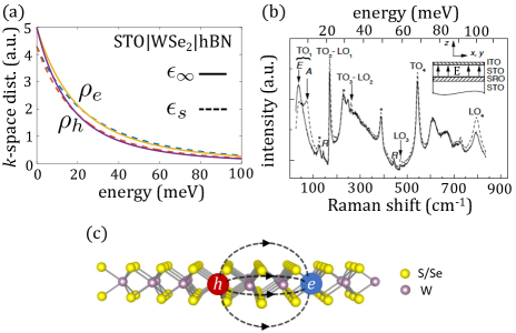
Figure 1: (a) k-space distributions of the electron and hole due to their relative motion in a charge-neutral exciton. (b) The optical phonon modes in STO, extracted from Raman spectra of 1 mm STO film at $T=5$ K without electric field (solid line) and when a field $E=2.2\times 10^{5}$ V/cm (dashed lines) is directed normal to the film plane. Taken from Ref. [40]. (c) Schematic of the electric field lines between the electron and hole of an exciton (dashed lines), some of which pass through the surrounding environments.

III Theory

The dynamical effects are obtained by solving the BSE through inclusion of the dynamical Coulomb interaction between charge particles. We first show how to incorporate the dynamical dielectric function in the potential and the way to obtain the dynamical self-energy of each component of the exciton. Then we use these quantities in the dynamical BSE.

III.1 Dynamical dielectric function

We start by considering the frequency dependence of the dielectric function of a general material subjected to a time-dependent periodic electric field of frequency $\omega$. The structure geometry will later be incorporated to obtain the effective dielectric function of the Coulomb interaction between charged particles in the monolayer.

Assuming a lossless Lorentzian oscillator model, the permittivity of ionic crystals under the effect of a periodic electric field is given by

$$\epsilon(\omega)=\epsilon_{\infty}\,\,\prod_{j}\frac{\omega_{j,\text{LO}}^{2}-\omega^{2}}{\omega_{j,\text{TO}}^{2}-\omega^{2}}.$$ (6)

The ratio between the static and high-frequency permittivities is the celebrated Lyddane–Sachs–Teller relation $\epsilon(\omega=0)/\epsilon(\omega=\infty)\equiv\epsilon_{0}/\epsilon_{\infty}=\prod_{j}\omega_{j,\text{LO}}^{2}/\omega_{j,\text{TO}}^{2}$. The index $j$ runs over the optical-phonon modes, where $\omega_{j,\text{LO/TO}}$ is the associated frequency of the longitudinal/transverse optical lattice vibration. Materials like TiO₂ and STO have several longitudinal and transverse modes such that $\omega_{j,\text{LO}}\simeq\omega_{j+1,\text{TO}}$. Figure 1(b) shows the phonon frequencies of STO with $\omega_{1,\text{LO}}=\omega_{2,\text{TO}}$, $\omega_{2,\text{LO}}=\omega_{3,\text{TO}}$, and $\omega_{3,\text{LO}}\simeq\omega_{4,\text{TO}}$. As a consequence, the frequency-dependent permittivity in Eq. (6) is mostly governed by the first and last modes, yielding

$$\epsilon(\omega)=\epsilon_{\infty}+\epsilon_{\infty}\frac{\omega^{2}_{4,\text{LO}}-\omega^{2}_{1,\text{TO}}}{\omega^{2}_{1,\text{TO}}-\omega^{2}}.$$ (7)

Based on this observation, we will use two unitless parameters to describe the dielectric response of each layer. The first parameter is the ratio between the first TO phonon energy and the estimated exciton binding energy

$$r_{1}=\frac{\hbar\omega_{1,\text{TO}}}{\varepsilon_{\text{X}^{0}}}.$$ (8)

We use $\varepsilon_{\text{X}^{0}}=170$ meV in this work (approximately the exciton binding energy in hBN-encapsulated WSe₂ [39, 12]). The second parameter is the square frequency ratio between the last LO mode and first TO mode

$$r_{2}=\frac{\epsilon_{0}}{\epsilon_{\infty}}=\frac{\omega^{2}_{N,\text{LO}}}{\omega^{2}_{1,\text{TO}}}.$$ (9)

The dielectric function in Eq. (7) can then be written as

$$\epsilon(\omega)=\epsilon_{\infty}\left(1+\frac{r_{2}-1}{1-\frac{\omega^{2}}{r^{2}_{1}\varepsilon_{\text{X}^{0}}^{2}}}\right).$$ (10)

The Coulomb interaction between charge particles in the monolayer is obtained by solving the Poisson Equation with the appropriate structure geometry. Details of the derivation are given in Ref. [39]. The dynamical Coulomb potential between charge particles is given by

$$V({\bf q},\omega)=\frac{2\pi e^{2}}{A\,\,\epsilon({\bf q},\omega)\,\,q},$$ (11)

where $A$ is the area of the system. Dynamical effects are incorporated through the dielectric functions of the surrounding dielectric materials, as detailed in Appendix A.

The dynamical Coulomb potential has singularities at the phonon frequencies. To circumvent this difficulty when solving the BSE or evaluating the self-energies, we use finite-temperature Green’s function formalism in which real frequencies are replaced by imaginary and discrete Matsubara frequencies [41]. Namely, $\epsilon({\bf q},\omega)$ is replaced with $\epsilon({\bf q},z-z^{\prime})$, where $z$ and $z^{\prime}$ are imaginary Matsubara energies of fermions before and after the interaction. Their discretized energy form is $(2\ell+1)\pi ik_{\text{B}}T$, where $\ell$ is an integer and T is temperature. Consequently, the positive real number $\omega^{2}$ in Eq. (10) is replaced by $(z-z^{\prime})^{2}$ which is a negative real number. Rather than having singularities, the dielectric function is now monotonously decaying from $\epsilon_{0}$ to $\epsilon_{\infty}$ as $z-z^{\prime}$ departs from 0.

III.2 Dynamical Self-Energy

The self-energy of an electron in the conduction ($c$) or valence band (v) is calculated from a self-consistent solution of the Dyson Equation

$$\Sigma_{i}({\bf k},z)=-\frac{1}{\beta}\sum_{{\bf q},z^{\prime}}G_{i}({\bf k-q},z^{\prime})V({\bf q},z-z^{\prime}).$$ (12)

where $\beta^{-1}=k_{B}T$, $i=\{\text{c,v}\}$, and the Green’s function is

$$G_{i}({\bf k},z) = \frac{G_{i}^{0}({\bf k},z)}{1-G_{i}^{0}({\bf k},z)\Sigma_{i}({\bf k},z)}$$ (13)

$$= \frac{1}{z-\varepsilon_{i}({\bf k})+\mu-\Sigma_{i}({\bf k},z)}.$$

${\bf k}$ and $\mu$ are the electron momentum and its chemical potential, respectively. $\varepsilon_{\text{c}}({\bf k})=E_{\text{g}}+{\hbar^{2}k^{2}}/{2m_{c}}$ is the energy dispersion of the electron in the conduction band and $\varepsilon_{\text{v}}({\bf k})={\hbar^{2}k^{2}}/{2m_{\text{v}}}$ is the corresponding one in the valence band.

We emphasize that it is important to include the dynamics in the Coulomb interaction and not only in the Green’s functions of the electron and hole. To illustrate this importance, we evaluate the self-energy by using a static potential $V({\bf q})$ instead of $V({\bf q},z-z^{\prime})$. Equation (12) in this case becomes frequency-independent $\Sigma({\bf k})=-\beta^{-1}\sum_{\bf q}V({\bf q})\sum_{z^{\prime}}G({\bf k+q},z^{\prime})\equiv\sum_{\bf q}V({\bf q})\left(f({\bf k+q})-\frac{1}{2}\right)$ where $f(k)$ is the Fermi-Dirac distribution function. In the zero-temperature limit and at charge neutrality, the self-energy of the electron in the conduction or valence bands is

$$\Sigma_{\text{c/v}}({\bf k})=\mp\frac{1}{2}\sum_{\bf q}V({\bf q}).$$ (14)

Namely, one gets a rigid energy shift of the bands which is essentially the BGR in the static limit. By neglecting dynamical effects in the potential, we lose the frequency dependence of the self-energies and decouple the electron self-energy from that of the hole (i.e., the electron and hole have independent self-energies which are identical to the ones of free particles in the bands). We will show later that the coupling and dynamical self-energies are important to get the correct energy blueshift of the exciton resonance, as observed in experiment [30].

One difficulty of self-energy calculations is the divergence of the sum over $\bf q$. We illustrate this point by using the non-dynamical BGR in Eq. (14). The 2D potential $V(q)$ scales as $q^{-2}$ in the short wavelength limit, resulting in a logarithmic divergence of the sum over $\bf q$. We circumvent this problem by choosing a reference TMD structure with respect to which energy shifts are calculated. Without loss of generality, we choose a reference system whose corresponding potential $V_{0}(q)$ is evaluated with the following fixed dielectric constants $\epsilon_{\text{t}}=\epsilon_{\text{b}}=3.8$. The BGR of a given system with respect to the reference system is then given by

$$\tilde{\Sigma}_{\text{c/v}}({\bf k}) = \mp\frac{1}{2}\sum_{\bf q}\left(V({\bf q})-V_{0}({\bf q})\right)$$ (15)

$$= \mp\frac{e^{2}}{2}\int_{0}^{\infty}dq\left(\frac{1}{\epsilon(q)}-\frac{1}{\epsilon^{0}(q)}\right).$$

$\epsilon(q)$ and $\epsilon^{0}(q)$ are the non-dynamical dielectric functions of the investigated TMD and reference system, respectively (see Eq. (27)). When dynamical effects are included, the self-energy in Eq. (12) has the same divergence problem, and it can be regularized in a similar way

$$\!\!\!\!\!\!\!\!\!\!\!\!\tilde{\Sigma}_{i}({\bf k},z) = -\frac{1}{\beta}\sum_{{\bf q},z^{\prime}}G_{i}({\bf k+q},z^{\prime})$$ (16)

$$\qquad\qquad\times\left[V({\bf q},z-z^{\prime})-V_{0}({\bf q})\right],\,\,\,\,\,\,\,\,\,\,\,\,\$$

where the free electron Green’s function now becomes

$$G_{i}({\bf k},z)=\frac{1}{z-\varepsilon_{i}({\bf k})+\mu-\tilde{\Sigma}_{i}({\bf k},z)}.$$ (17)

The dynamical self-energy $\tilde{\Sigma}_{i}({\bf k},z)$ can be self-consistently calculated from Eqs. (16) and (17) using the iterative method (see Appendix B for details).

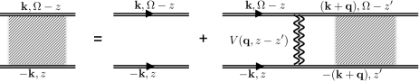
Figure 2: Feynman diagram for the Bethe-Salpeter Equation describing the interaction between electron (top double lines) and hole (bottom double lines) via the dynamical potential $V({\bf q},z-z^{\prime})$, represented by the doubled wavy line.

III.3 Dynamical Bethe-Salpeter Equation

The BSE is an equation for bound states between two particles. Its dynamical version is used here to describe the interaction between electron and hole excited by light with negligible momentum. The equation with its Feynman diagram shown in Fig. 2 reads [32, 31, 42]

$$\!\!\!\!\!\!\!\!\!\!\!\!G({\bf k},z,\Omega)=G^{0}({\bf k},z,\Omega)\,\,\,+$$ (18)

$$\,\,\,\,\frac{1}{\beta}\sum_{{\bf q},z^{\prime}}G^{0}({\bf k},z,\Omega)V({\bf q},z-z^{\prime})G({\bf k+q},z^{\prime},\Omega),$$

where the Green’s function of a free electron-hole pair is given by

$$G^{0}({\bf k},z,\Omega) = \frac{1}{\Omega-z-\varepsilon_{\text{c}}({\bf k})-\tilde{\Sigma}_{\text{c}}({\bf k},\Omega-z)+\mu}$$ (19)

$$\,\times\frac{1}{z+\varepsilon_{\text{v}}({\bf k})+\tilde{\Sigma}_{\text{v}}({\bf k},z)-\mu}.$$

$\Omega$, an even (bosonic) imaginary Matsubara energy, is related to the energy of the photon exciting the electron-hole pair. Equation (18) can be solved using the iterative method, the same method as the one used for calculating the self-energies in Eqs. (16)-(17). The details are presented in Appendix B. One can notice that solutions of different bosonic frequencies $\Omega$ are decoupled, and therefore, equations of different $\Omega$s can be solved independently. The solutions are then used to find the contracted pair function

$$g({\bf k},\Omega)=-\beta^{-1}\sum_{z}G({\bf k},z,\Omega).$$ (20)

The final step is to analytically continue the contracted pair function to the real-frequency axis, $g({\bf k},\Omega\rightarrow\omega+i\delta)$, using the Padé approximation technique [42, 32, 43], as discussed in Appendix C. The real-frequency pair function is related to optical absorption by

$$\text{A}(\omega)=-\sum_{{\bf k}}\text{Im}\left[g({\bf k},\Omega\rightarrow\omega+i\delta)\right],$$ (21)

where $\delta$ is broadening parameter which might include effects of finite exciton lifetime, scattering off impurities, and thermal fluctuations. Note that temperature in this formalism sets the energy resolution of Matsubara frequencies and is not related to the broadening of resonance peaks which is controlled by $\delta$. In this work, we keep $\delta=3$ meV for the sake of simplicity. More details are mentioned in Appendix E.

In the non-dynamical regime, the potential and self-energies are frequency independent. The BSE in Eq. (18) can be further contracted, yielding

$$\!\!\!g({\bf k},\Omega)=g^{0}({\bf k},\Omega)-\sum_{{\bf q}}g^{0}({\bf k},\Omega)\,\,V({\bf q})\,\,g({\bf k+q},\Omega),$$ (22)

and the corresponding function of a free electron-hole pair is given by [41, 31]

$$g^{0}({\bf k},\Omega) = -\beta^{-1}\sum_{z}G^{0}({\bf k},z,\Omega)$$ (23)

$$= \frac{f_{\text{v}}({\bf k})-f_{\text{c}}({\bf k})}{\Omega+\varepsilon_{\text{v}}({\bf k})+\tilde{\Sigma}_{\text{v}}({\bf k})-\varepsilon_{\text{c}}({\bf k})-\tilde{\Sigma}_{\text{c}}({\bf k})}.\,\,\,\,\,\,\,\,\,\,\,\,\,\,$$

$f_{\text{c(v)}}({\bf k})$ is the Fermi-Dirac distribution function for electrons in the conduction (valence) band. Note that the free-pair function has the same form as the polarization function in the random-phase approximation. The only difference is that we have interband electron-hole excitation here instead of intraband particle-hole excitation in the polarization function. The analogy means that the method developed in this work is applicable for studying the dynamical response in the dielectric screening formalism.

IV RESULTS AND DISCUSSIONS

We first show signatures of dynamical effects in the BGR and in self-energies of free particles. The self-energies are then used in calculations of the pair function $g({\bf k},\Omega)$, which in turn is used to extract the spectral position of the charge-neutral exciton resonance.

IV.1 Dynamical effects in the self-energy and BGR

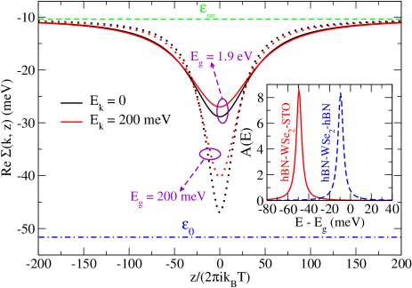
Figure 3: Real part of the self-energy $\Sigma_{\text{c}}({\bf k},z)$ of conduction-band electrons in hBN-WSe₂-STO as a function of Matsubara frequency $z=(2\ell+1)\pi ik_{\text{B}}T$. Solid (dotted) lines are self-consistent solutions of Eqs. (16)-(17) when $E_{g}=1.9$ eV (0.2 eV). For comparison, the dashed (dash-dotted) line is the solution of Eq. (15) with $\epsilon_{\infty}$ ($\epsilon_{0}$). Inset: Spectral function of an electron at the edge of the conduction band, $E_{k}=0$, in hBN-WSe₂-STO (red solid line) and hBN-WSe₂-hBN (blue dashed line). The resonance energy of the latter (former) emerges at $-9.5$ meV ($-49.5$ meV), denoting the BGR with respect to the edge of the conduction band in the non-dynamical reference system ($\epsilon_{\text{b}}=\epsilon_{\text{t}}=3.8$).

Figure 3 shows the self-energy of electrons $\Sigma_{\text{c}}({\bf k},z)$ as a function of Matsubara frequency $z$ for two representative energies, $E_{\bf k}={\hbar^{2}k^{2}}/{2m_{\text{c}}}=\{0,200\text{ meV}\}$. Dynamical effects are included by using the potential $V(q,z-z^{\prime})$ in Eq. (11) adjusted to describe WSe₂ monolayer between STO and hBN layers. The parameters used in the calculation are listed in Appendix D. The bandgap energies in these calculations are $E_{\text{g}}=1.9$ eV (solid lines) and $E_{\text{g}}=0.2$ eV (dotted lines), where the chemical potential is set at the midgap, i.e., $\mu=E_{\text{g}}/2$. The corresponding self-energies in the valence band, $\Sigma_{\text{v}}({\bf k},z)$, are almost the same as $\Sigma_{\text{c}}({\bf k},z)$ but with opposite sign (not shown). This similarity is reasoned by similar effective masses of electrons and holes, which together with the midgap chemical potential, result in a good electron-hole symmetry. The self-energy is used to obtain the electron Green’s function $G_{\text{c}}({\bf k},z)$ through Eq.(17). The conduction-band BGR is evaluated from the resonance energy of the spectral function

$$A(E)=-\text{Im}\left[G_{\text{c}}({\bf k}=0,z\rightarrow E+i\delta)\right].$$ (24)

The analytical continuation from imaginary to real energies $(z\rightarrow E)$ is performed by using the Padé approximation technique (see Appendix C).

The inset of Fig. 3 shows the spectral functions $A(E)$ at the edge of the conduction band, $k=0$, in hBN-WSe₂-STO and hBN-WSe₂-hBN structures when dynamical effects are included. The resonance emerges at the conduction-band edge, where the zero energy level corresponds to the edge of the conduction band in the non-dynamical reference system ($\epsilon_{\text{t}}=\epsilon_{\text{b}}=3.8$). Table 1 summarizes the BGR calculations using low- and high-frequency dielectric constants as well as the dynamical dielectric function. The dynamical result is very close to the one calculated with $\epsilon_{0}$, providing strong evidence that charge particles in the monolayer are also screened by phonons. On the other hand, the self-energies $\Sigma_{\text{c}}({\bf k},z)$ shown by solid lines in Fig. 3 are closer to the self-energy calculated by Eq. (14) with $\epsilon_{\infty}$ (dashed line). This resemblance comes from the inclusion of the bandgap energy $E_{\text{g}}$. This inclusion does not affect the BGR because after analytical continuation $z\rightarrow E_{\text{g}}+E$ in Eq. (24), the bandgap energy in the denominator of Eq. (17) is eliminated (i.e., it is merely a reference energy level).

Table 1: BGR calculations with different dielectric parameters. The energies shifts are with respect to the reference system (hBN-WSe₂-hBN with $\epsilon(\omega)=\epsilon_{\infty}$ in the hBN layers).

	hBN-WSe2-STO	hBN-WSe2-hBN
$\epsilon(\omega)$	$-49.5$ meV	$-9.5$ meV
$\epsilon_{0}$	$-51.6$ meV	$-10.9$ meV
$\epsilon_{\infty}$	$-10.4$ meV	$0$ meV

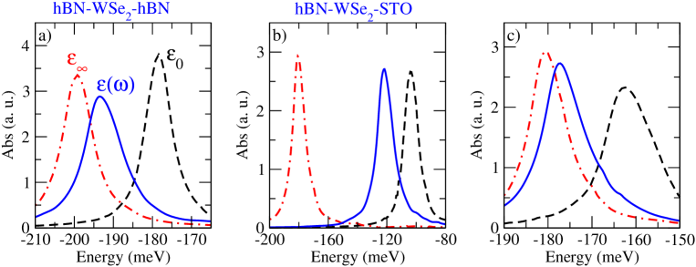
Figure 4: Absorption spectra of (a) hBN-WSe₂-hBN and (b) hBN-WSe₂-STO structures. Blue solid lines are results calculated with the dynamical potential $V({\bf q},\omega)$ but without self-energies of the electron and hole in the exciton. Black dashed lines (red dash-dotted lines) are respective results with the non-dynamical potential $V({\bf q})$ when using $\epsilon_{0}$ ($\epsilon_{\infty}$). (c) Results of the same calculations as in (b) but when modeling the STO layer with $r_{2}=1.3$ instead of 4096.

IV.2 Dynamical effects in the optical spectrum

The dynamical potential $V({\bf q},z-z^{\prime})$ affects both the BGR and binding energy. To decouple these effects, we focus first on the binding energy by neglecting the self-energy terms in the BSE (i.e., $\tilde{\Sigma}_{\text{c/v}}({\bf k},z)=0$ in Eq. (18)). The resulting absorption spectra of hBN-WSe₂-hBN and hBN-WSe₂-STO structures are shown in Figs. 4(a) and (b), respectively. For comparison, we have also calculated the absorption spectra with the non-dynamical potential $V({\bf q})$ using low-frequency dielectric constants (dashed lines) and high-frequency ones (dash-dotted lines). The exciton binding energy is $E_{\text{b}}=122$ meV when using the dynamical potential in hBN-WSe₂-STO. Corresponding values of the non-dynamical calculations are $E_{\text{b}}^{0}=104$ meV and $E_{\text{b}}^{\infty}=181$ meV. The dynamical binding energy is closer to the one calculated with $\epsilon_{0}$, meaning that screening of the interaction between the electron and hole is dominated by the low frequency part of the dielectric function. On the other hand, Fig. 4(a) shows opposite trend for the hBN-WSe₂-hBN structure, where the dynamical calculation is closer to the non-dynamical one calculated with $\epsilon_{\infty}$.

To understand this behavior, we define a low-frequency contribution factor

$$\alpha\equiv\frac{E^{\infty}_{b}-E_{\text{b}}}{E^{\infty}_{b}-E^{0}_{\text{b}}},$$ (25)

where $\alpha=1$ ($\alpha=0$) means that the exciton binding is completely controlled by $\epsilon_{0}$ ($\epsilon_{\infty}$). Using the calculated results in Fig. 4, the low-frequency contribution factor is $\alpha=0.77$ for hBN-WSe₂-STO and $\alpha=0.27$ for hBN-WSe₂-hBN. The difference stems from the Lyddane–Sachs–Teller relation of hBN and STO, expressed through the parameter $r_{2}$ in Eq. (9). A larger $r_{2}$ leads to stronger dynamical contribution in Eq. (10), which in turn pushes the dielectric function away from $\epsilon_{\infty}$ and closer to $\epsilon_{0}$. Indeed, $r_{2}>10^{3}$ in low-temperature STO versus $r_{2}\approx 1.3$ in hBN. To confirm that our understanding is correct, we repeated the calculation of hBN-WSe₂-STO but with changing $r_{2}$ of STO from $4096$ to $1.3$. This change corresponds to lowering $\epsilon_{0}$ of STO from $25000$ to $7.8$. The result of the calculation is shown in Fig. 4 (c). We obtain $\alpha=0.2$, confirming that the contribution of $\epsilon_{\infty}$ is indeed dominant at smaller $r_{2}$.

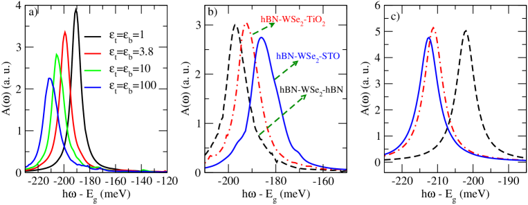
Figure 5: (a) Calculated absorption spectra with the non-dynamical potential of various dielectric environments. The BGR effect is calculated with respect to the reference system ($\epsilon_{b}=\epsilon_{t}=3.8$). The exciton resonance shows energy redshift when the dielectric screening is increased. (b) Calculated absorption spectrum with the dynamical potential and $E_{\text{g}}=1.9$ eV. The exciton resonance shows energy blueshift when the dielectric screening of the environment is increased. (c) The same as in (b) but for $E_{\text{g}}=0.2$ eV, showing an energy redshift trend.

Next, we include the self-energy in calculations of the absorption spectra and consider the competition between BGR and binding energy. The exciton resonance energy is the difference between band-gap energy and electron-hole binding energy, $E_{X_{0}}=E_{g}-E_{b}$. When the dielectric environment surrounding the monolayer or quantum well changes, the renormalized bandgap and binding energies tend to offset each other, such that $E_{X_{0}}$ is only slightly changed [31, 28, 32]. For example, a stronger dielectric screening leads to smaller band-gap energy and smaller binding energy, where their difference is much smaller than the change of each of them. As mentioned in Sec. II, a common observation in monolayer semiconductors is a small overall energy redshift of $E_{X_{0}}$ when the materials that encapsulate the monolayer are replaced with higher-dielectric constant materials. Figure 5(a) shows the calculated absorption spectra from the BSE using a non-dynamical potential. The BGR effect is calculated with respect to the reference system ($\epsilon_{b}=\epsilon_{t}=3.8$). In accordance with the analysis of Sec. II, the exciton resonance redshifts when the dielectric constant of the surrounding environment increases.

Yet, the energy redshift can turn to a blueshift if dynamical effects are considered through the potential $V({\bf q},z-z^{\prime})$ and self-energies $\tilde{\Sigma}_{\text{c/v}}({\bf k},z)$, and if replacing the encapsulating materials involve a large change in $\epsilon_{0}$ and a small change in $\epsilon_{\infty}$. Figure 5(b) shows the resulting absorption spectra of three different structures: hBN-WSe₂-hBN, hBN-WSe₂-TiO₂, and hBN-WSe₂-STO. In agreement with experimental results [30], replacing the supporting hBN layer with TiO₂ leads to energy blueshift, which is further increased when STO is used as support. The opposite energy-shift trends of the non-dynamical and dynamical calculations in Figs. 5(a) and (b), can be explained as follows. The binding energy is mainly dominated by the low-frequency part of the dielectric function, where the change is from $\epsilon^{\text{hBN}}_{0}=4.9$ to $\epsilon^{\text{TiO}_{2}}_{0}\sim 200$ and then to $\epsilon^{\text{STO}}_{0}=25000$. As a result, the change in binding energy is relatively significant. On the other hand, the self-energies of the electron and hole in the exciton have larger contribution from the high-frequency part, where the change is from $\epsilon^{\text{hBN}}_{\infty}=3.8$ to $\epsilon^{\text{TiO${}_{2}$}}_{\infty}\sim\epsilon^{\text{STO}}_{\infty}\sim 6$. As a result, the BGR effect is relatively mitigated. The confluence of both trends is that the energy redshift from BGR is smaller than the energy blueshift from binding energy ($\Delta E_{\text{g}}<|\Delta E_{\text{b}}|$), leading to overall energy blueshift of the exciton resonance.

We provide mathematical and physical reasonings to the observed energy blueshift (i.e., why weakening of the binding energy is stronger than the bandgap-energy shrinkage). As shown by Eq. (19), the self-energy of the electron in the exciton is associated with $(\Omega-z)$ whereas that of the hole with $z$. The bosonic frequency $\Omega$ is related to the photon energy which is of the order of the bandgap energy; a large value compared with phonon or binding energies. Consequently, the self-energy of at least one of the exciton’s components asymptotically approaches the value of the self-energy when calculated non-dynamically with $\epsilon_{\infty}$. An alternative view is that the energy difference between the exciton components is encoded as a time-dependent phase factor $\exp(iE_{g}t/\hbar)$, which leads to a dominant contribution from the high-frequency part of the dielectric function to the exciton’s BGR.

Finally, we recall that the edge of an energy band is merely a reference level when the interest is in the BGR of a charge particle in this band. The energy reference level is eliminated in the analytical continuation step (see discussion at the end of Sec. IV.1). Therefore, the dominant contribution to the BGR of a charge particle comes from the low-frequency part of the dielectric function (Table 1). On the other hand, the reference energy level for a bound pair (exciton) mandates that at least its electron or hole are subjected to high frequencies that cannot be eliminated by analytical continuation. To confirm the importance of the bandgap energy, we have performed additional calculations with similar parameters to the ones used in Fig. 5(b), but with a much smaller bandgap energy, $E_{\text{g}}=0.2$ eV. The results are shown in 5(c). As expected from the explanation above, the trend is now reversed and we observe a small energy redshift coming from lesser contribution of high frequencies to the BGR (Fig. 3).

V Summary

We have presented a model that incorporates dynamical dielectric screening effects in the Bethe-Salpeter Equation. The model allows one to study excitons in transition-metal dichalcogenide monolayers that are embedded in various dielectric environments. We have employed an iterative numerical technique to solve the Bethe-Salpeter Equation, allowing us to perform comprehensive calculations with a large number of Matsubara frequencies and fine mesh in momentum space. The theory sheds light on the intricate energy shifts of exciton resonances. Assuming that the bandgap energy is evidently larger than the exciton binding energy, we can have one of two opposite trends when the materials on top and/or below the monolayer are replaced with higher-dielectric constant materials. If the involved materials are such that their low- and high-frequency dielectric constants are not evidently different ($\epsilon_{0}/\epsilon_{\infty}\not\gg 1$), then we should expect the exciton energy to redshift in the new environment. On the other hand, the exciton energy should blueshift if $\epsilon_{0}/\epsilon_{\infty}\gg 1$. These findings, identified by the inclusion of dynamical dielectric screening, help us to explain recent measurements in hBN-TMD-hBN, hBN-TMD-TiO₂, and hBN-TMD-STO devices [30].

Beyond the agreement of the theory with experiment, the analysis identifies a distinction between the bandgap energy renormalization of excitonic complexes and the energy renormalization of free electrons in the conduction band or free holes in the valence band. In the excitonic case, the renormalization has important contribution from the high-frequency part of the dielectric function. On the other hand, energy renormalizations of free electrons in the conduction band and/or free holes in the valence band are dominated by the low-frequency part of the dielectric function. One important consequence is that if $\epsilon_{0}$ and $\epsilon_{\infty}$ are much different, the bandgap energy renormalization that one measures in ARPES experiments cannot be used to infer the bandgap energy renormalization of bound electron-hole pairs.

Appendix A Coulomb potential

We simulate the structure geometry as a TMD monolayer with thickness $d$ sandwiched between top and bottom layers with dielectric constants $\epsilon_{\text{t}}$ and $\epsilon_{\text{b}}$. The TMD monolayer is modeled as three atomic sheets with polarizabilities $\chi_{+}$ for the central Tungsten (W) sheet and $\chi_{-}$ for the top and bottom Selenium (Se) ones, displaced by $\pm d/4$ from the center. The model was developed in Ref. [39] and has been employed to study several problems [25, 26, 44]. The resulting static potential for the interaction between two charges in the monolayer is

$$V(q)=\frac{2\pi e^{2}}{A\,\,\epsilon(q)\,\,q},$$ (26)

where the dielectric function reads

$$\epsilon(q)=\frac{1}{2}\left[\frac{N_{t}(q)}{D_{t}(q)}+\frac{N_{b}(q)}{D_{b}(q)}\right].$$ (27)

Defining $p_{j}\equiv(\epsilon_{j}-1)/(\epsilon_{j}+1)$ for the top and bottom dielectric constants ($j=b/t$), we get that

$$D_{j}(q) = 1+q\ell_{-}-q\ell_{-}(1+p_{j})\text{e}^{-\frac{qd}{2}}-(1-q\ell_{-})p_{j}\text{e}^{-qd},$$

$$N_{j}(q) = \left(1+q\ell_{-}\right)\left(1+q\ell_{+}\right)$$ (28)

$$+ \left[\left(1-p_{j}\right)-\left(1+p_{j}\right)q\ell_{+}\right]q\ell_{-}\text{e}^{-\frac{qd}{2}}$$

$$+ (1-q\ell_{-})(1-q\ell_{+})p_{j}\text{e}^{-qd}.$$

where $\ell_{\pm}=2\pi\chi_{\pm}$.

The Coulomb potential in Eq. (26) becomes frequency dependent by using dynamical polarization parameters, $p_{j}(\omega)\equiv(\epsilon_{j}(\omega)-1)/(\epsilon_{j}(\omega)+1)$, where $\epsilon_{j}(\omega)$ is the dielectric function of the $j=b/t$ layer (Eq. (10)).

Appendix B Iterative method

The iterative method is used in calculations of Eqs. (16)-(18). These equations can generally be written as

$$\Gamma({\bf k},z)=\frac{1}{\beta}\sum_{{\bf q},z^{\prime}}F\left(z,\Gamma({\bf k+q},z^{\prime})\right),$$ (29)

where $\Gamma({\bf k},z)$ represents either the self-energy $\tilde{\Sigma}_{i}({\bf k},z)$ in Eqs. (16)-(17) or the interacting pair Green’s function $G({\bf k},z,\Omega)$ in Eq. (18). We have omitted the bosonic frequency $\Omega$ in Eq. (29) because the BSE of different $\Omega$ parameters are decoupled and can be solved separately. When we are interested in self-energies, $F\left(z,\Gamma({\bf k+q},z^{\prime})\right)$ is a composite function of the form

$$F\left(z,\Gamma({\bf k+q},z^{\prime})\right)=\frac{V_{0}({\bf q})-V({\bf q},z-z^{\prime})}{{z-\varepsilon_{i}({\bf k+q})+\mu-\Gamma({\bf k+q},z)}}\,\,\,\,\,\,\,\,\,\,\,\,\,\,\,$$ (30)

with $\Gamma({\bf k},z)\equiv\tilde{\Sigma}_{i}({\bf k},z)$. And when interested in the BSE

$$F\left(z,\Gamma({\bf k+q},z^{\prime})\right) = G^{0}({\bf k},z,\Omega)\,\,\left[\beta\delta_{\bf q,0}\delta_{z,z^{\prime}}\right.$$ (31)

$$+ \left.V({\bf q},z-z^{\prime})\Gamma({\bf k+q},z^{\prime},\Omega)\right]\,\,\,\,\,\,\,\,\,\,\,\,\,\,\,\,\,\,$$

with $\Gamma({\bf k},z)\equiv G({\bf k},z,\Omega)$.

The computational cost can be greatly reduced if one considers a two-dimensional system with circular symmetry in momentum space $\bf k$, i.e., $\Gamma({\bf k},z)\equiv\Gamma(k,z)$. Equation (29) then becomes

$$\!\!\!\!\!\Gamma(k,z)=\sum_{z^{\prime}}\int_{0}^{\infty}\frac{A\,\,dq}{4\pi^{2}}\int_{0}^{\pi}F\left(z,\Gamma({\bf k+q},z^{\prime})\right)d\theta.\,\,\,$$ (32)

The equation is solved numerically by discretizing the momentum space, i.e., we calculate $\Gamma(k_{i},z)$ at $n_{K}$ representative momenta $\{k_{i}=\left(i-\frac{1}{2}\right)dk,i=\overline{1,n_{K}}\}$ and $n_{Z}$ fermionic Matsubara frequencies. Here, we divide the momentum space to $n_{K}$ rings with similar thickness $dk=K_{\text{Max}}/n_{K}$ where the cutoff momentum $K_{\text{Max}}$ is chosen large enough to neglect contributions from states above such momentum. The cutoff energy corresponding to $K_{\text{Max}}$ is $E^{k}_{\text{Cut}}$. The number of Matsubara frequencies $n_{Z}$ involved in the calculation guarantees that $E^{z}_{\text{Cut}}=n_{Z}\times\pi k_{\text{B}}T$ is out of the accessible range of all related energy quantities of the considered phenomena (e.g., bandgap energy of the TMD monolayer, exciton binding energy, and kinetic energies of the electron and hole in the exciton).

For $({\bf k}_{i}+{\bf q})$ in Eq. (32) to fall into the $j^{\text{th}}$ ring, we set the condition

$$\mathcal{C}_{i,j}:\,\,\,\left(j-1\right)\leq\frac{\sqrt{q^{2}+k^{2}_{i}+2k_{i}q\cos\theta}}{dk}<j.$$ (33)

Using this condition, we can rewrite Eq. (32) in a form suitable for numerical calculation

$$\Gamma(k_{i},z)=\sum_{z^{\prime},j}\mathcal{F}_{i,j}(z,z^{\prime})\,\,,\,\,\,\,$$ (34)

where the function $\mathcal{F}_{i,j}(z,z^{\prime})$ is defined by

$$\mathcal{F}_{i,j}(z,z^{\prime})=\frac{A}{4\pi^{2}}\int_{\{q,\theta\}\in\mathcal{C}_{i,j}}F\left(z,\Gamma({\bf k}_{i}+{\bf q},z^{\prime})\right)dqd\theta.\,\,\,\,\,\,\,\,\,\,\,\,$$ (35)

This equation can be solved by matrix inversion [42, 32]. However, the computational cost of such calculation is expensive and prohibits the use of a large number of Matsubara frequencies and fine momentum mesh. Instead, we use an iterative method which helps to solve Eq. (34) at a much smaller computational cost. The iterative steps are

1. Start by guessing a solution, usually the non-interacting function $\Gamma_{\text{in}}(k_{i},z)\equiv\Gamma^{0}(k_{i},z)$.

2. Substitute the input function $\Gamma_{\text{in}}(k_{i},z)$ into the right hand side of Eq. (34) to find the output function $\Gamma_{\text{out}}(k_{i},z)$ on the left hand side.

3. Use $\Gamma_{\text{out}}(k_{i},z)$ as an input to the right-hand side of Eq. (34) repeatedly until convergence is reached (i.e., $\Gamma_{\text{out}}(k_{i},z)=\Gamma_{\text{in}}(k_{i},z)$).

In calculation of the interacting pair Green’s function $G({\bf k},z,\Omega)$, the iterative procedure can be performed for each Matsubara frequency $\Omega=\Omega_{j}$ independently. The convergence of the iterative method can be sped up by using the converged results of the higher frequency $G({\bf k},z,\Omega_{j})$ as the initial trial function for the next lower frequency $G_{\text{in}}({\bf k},z,\Omega_{j-1})\equiv G({\bf k},z,\Omega_{j})$.

The converged solution of the BSE equation is difficult to obtain for low values of $\Omega_{j}$. Fortunately, we can get rid of the the first few lowest $\Omega_{j}$ frequencies because their Green’s functions only contribute to states close to the continuum (e.g., 2$s$, 3$s$, and so on). The 1$s$ exciton state, with binding energy of hundreds of meV, is mostly controlled by high values of $\Omega_{j}$. The convergence of the analytical continuation depends on the number of bosonic frequencies, $n_{\Omega}$, as discussed in Appendix E. In addition, convergence of the iterative method for the BSE can be improved by lowering the change from the input to output Green’s functions. This can be done by modifying the third step above, where instead of directly using the output Green’s function, $G_{\text{out}}({\bf k},z,\Omega_{j})$, we use a linear combination of the old input and output Green’s functions as input for the next iterative step

$$\eta G_{\text{in}}({\bf k},z,\Omega_{j})+(1-\eta)G_{\text{out}}({\bf k},z,\Omega_{j})\rightarrow G_{\text{in}}({\bf k},z,\Omega_{j}).\,\,\,\,\,\,\,\,\,\,\,\,\,\,$$ (36)

The calculations in this work use $\eta=0.5$.

One useful property is that the contracted exciton Green’s function obeys

$$g({\bf k},-\Omega)=g^{*}({\bf k},\Omega),$$ (37)

thereby saving half the computational effort by calculating $g({\bf k},\Omega)$ for positive Matsubara frequencies and using the above relation to find $g({\bf k},\Omega)$ of negative Matsubara frequencies.

Once the self-energy $\tilde{\Sigma}_{i}({\bf k},z)$ and the contracted exciton pair function $g({\bf k},\Omega)$ are obtained, the Padé approximation technique is employed to extract the BGR and absorption spectrum, respectively.

Appendix C Padé approximation technique

Padé approximation is a technique used to perform analytical continuation from imaginary Matsubara energies to real ones [42, 32, 43]. Usually the method is used for finding the real frequency Green’s function when its values $\{G_{i}\}$ are known at $N$ Matsubara frequencies $\{z_{i}\}$ (or $\{\Omega_{i}\}$ in case of bosonic Green’s functions), where $i=\overline{1,N}$. In this work, the Green’s function is obtained from Eqs. (17) or (20). To perform the continuation, we look for the Green’s function of each momentum $\bf k$ in form of a rational fraction

$$G_{N}(z)=\cfrac{a_{1}}{1+\cfrac{a_{2}(z-z_{1})}{1+\cfrac{a_{3}(z-z_{2})}{1+\cdots\cfrac{\vdots}{\cfrac{\vdots}{1+\cfrac{a_{N}(z-z_{N-1})}{1}\,\,,}}}}}$$ (38)

where the coefficients $a_{i}$ are to be determined so that

$$G_{N}(z_{i})=G_{i};\quad i=\overline{1,N}.$$ (39)

If one defines a set of functions $\{f_{j}(z)\}$ for $j=\overline{1,N}$ by the following recursion

$$f_{1}(z_{i}) = G_{i};\quad\mbox{for}\quad i=\overline{1,N}$$

$$f_{j}(z) = \frac{f_{j-1}(z_{j-1})-f_{j-1}(z)}{(z-z_{j-1})f_{j-1}(z)},$$ (40)

the coefficients $a_{i}$ in Eq. (38) are given by

$$a_{i}=f_{i}(z_{i})\quad\mbox{for}\quad i=\overline{1,N}.$$ (41)

Indeed, the recursion in Eq .(40) leads to

$$f_{j-1}(z)=\frac{f_{j-1}(z_{j-1})}{1+(z-z_{j-1})f_{j}(z)},$$ (42)

which means that

$$f_{1}(z) = \frac{f_{1}(z_{1})}{1+(z-z_{1})f_{2}(z)}.$$ (43)

The condition of $f_{1}(z_{1})=G_{1}=G_{N}(z_{1})$ from Eqs. (39)-(40) leads to $a_{1}=f_{1}(z_{1})$. Applying the recursion in Eq. (42) one more time, we have

$$f_{1}(z)=\frac{a_{1}}{1+(z-z_{1})\frac{f_{2}(z_{2})}{1+(z-z_{2})f_{3}(z)}},$$ (44)

which can be combined with the condition of $f_{1}(z_{2})=G_{2}=G_{N}(z_{2})$ from Eqs. (39)-(40) to prove that $a_{2}=f_{2}(z_{2})$. The same procedure can be performed with higher indices to prove Eq. (41).

The introduction of the recursive relation in Eq. (40) supports the calculation of the coefficients $\{a_{i}\}$ through the following steps

• Start with $f_{1}(z_{i})=G_{i}$ for $i=\overline{1,N}$.

• Express $f_{j}(z_{i})$ of higher indices $j>1$ by assigning $z=z_{i}$ in Eq. (40).

• Obtain $a_{i}$ from Eq. (41).

The real-frequency Green’s function is obtained from Eq. (38) by replacing $z$ with $\omega+i\delta$, where the broadening parameter $\delta$ takes into account effects of finite lifetimes, scattering off impurities, and thermal fluctuations.

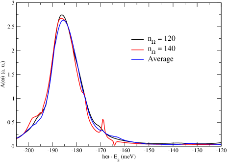
Figure 6: An example of using the analytical continuation to obtain the absorption spectrum of hBN-WSe₂-STO structure. The black and red lines are absorption spectra obtained from the Padé approximation using $N\equiv n_{\Omega}=120$ and 140 points, respectively. The spurious noise is suppressed by averaging the absorption spectra of different $n_{\Omega}$s (see text).

Figure 6 shows the absorption spectra obtained from the Padé approximation using $N\equiv n_{\Omega}=120$ (black line) and $n_{\Omega}=140$ (red line) points, corresponding to 40 and 20 neglected Matsubara frequencies around $\Omega=0$, respectively. Other parameters are provided in Appendix D. Because the technique employs the rational fraction in Eq. (38) to approximate the Green’s function, it inherently introduces noises in form of random and weak spurious peaks other than the main broad peak of the exciton bound state. The latter emerges at the same spectral position for all values of $n_{\Omega}$. Averaging the spectra of different $n_{\Omega}$s helps to suppress the spurious peaks. The results shown in this work are averages of spectra calculated with $n_{\Omega}=\{120,122,124,...140\}$.

Appendix D Parameters

The following parameters are used for the WSe₂ monolayer in different dielectric environments.

1. The effective masses are $m_{c}=0.29m_{0}$ (top conduction-band valley), $m_{\text{v}}=0.36m_{0}$ (top valence-band valley) [45]. The kinetic energies of electrons and holes are evaluated by parabolic energy dispersion.

2. The monolayer parameters of the potential are $d=$ 6 $\AA$ and $\ell_{+}=\ell_{-}=5d$ (Appendix A).

3. The dielectric constants of hBN, TiO₂, and STO, and the parameter $r_{1}=\hbar\omega_{\text{TO}}/\varepsilon_{\text{X}^{0}}$ (with $\varepsilon_{\text{X}^{0}}=170$ meV) are listed in Table 2.

   Table 2: Parameters of different dielectric environments.

   Materials	hBN	TiO2	STO
   $\epsilon_{0}$	4.9 [39, 46, 47]	192 [36, 48]	25000 [34, 35]
   $\epsilon_{\infty}$	3.8 [39, 46, 47]	6 [48]	6 [35]
   $r_{1}$	0.55 [46]	0.14 [48]	0.1 [49, 50, 40]

4. The following parameters are used in the numerical calculations of the self-energy and BSE: $n_{K}=100$, $E^{k}_{\text{Cut}}=2$ eV, $n_{Z}=3200$, T = 80 K, and the broadening used in the analytical continuation of Eq. (21) and (24) is $\delta=3$ meV.

Appendix E Numerical aspects

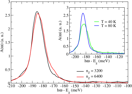
Figure 7: Calculated absorption spectra with $n_{Z}=3200$ and $6400$ fermionic Matsubara frequencies. Inset: Calculated absorption spectra at $T=40$ K and $80$ K.

The temperature enters the BSE (Eq. (18)) via the imaginary Matsubara frequencies, classified as bosonic $\Omega=2\ell\pi ik_{\text{B}}T$ (exciton) or fermionic $z=(2\ell+1)\pi ik_{\text{B}}T$ (electron and hole). Due to computational limitation, the calculation includes a finite number of fermionic frequencies $n_{Z}$ which, as mentioned in Appendix B, is chosen to guarantee a very large $E^{z}_{\text{Cut}}$. All the calculations in this work are performed with $n_{Z}=3200$ and $T=80$ K, corresponding to $E^{z}_{\text{Cut}}\simeq 70$ eV which is far larger than the bandgap and exciton binding energy of the system.

The converged solutions are shown by the inset of Fig. 7 in which we compare the results for T = 40 K and T = 80 K. While doubling the temperature somewhat affects the resonance amplitudes, it hardly changes the resonance energy (we only care for the exciton energy in this work). Doubling the number of fermionic frequencies, $n_{Z}$ as shown in Fig. 7, hardly affects the height and spectral position of the peak, meaning that the calculation is converged with $T=80$ K and $n_{Z}=3200$.

It is emphasized that the temperature $T$ sets the energy resolution of the discrete Matsubara frequencies, while it does not contribute to the broadening of the resonance peak. The temperature-dependent broadening, as seen in experiments, can be modeled through the broadening parameter $\delta(T)$. We have used $\delta=3$ meV throughout this work, neglecting its temperature dependence for simplicity.

References

- [1] D. Xiao, G.-B. Liu, W. Feng, X. Xu, and W. Yao, Coupled spin and valley physics in monolayers of MoS2 and other group-VI dichalcogenides, Phys. Rev. Lett. 108, 196802 (2012).
- [2] K. F. Mak, C. Lee, J. Hone, J. Shan, and T. F. Heinz, Atomically thin MoS2: A new direct-gap semiconductor, Phys. Rev. Lett. 105, 136805 (2010).
- [3] A. Splendiani, L. Sun, Y. Zhang, T. Li, J. Kim, C.-Y. Chim, G. Galli, and F. Wang, Emerging photoluminescence in monolayer MoS2, Nano Lett. 10, 1271 (2010).
- [4] J. Cai, E. Anderson, C. Wang, X. Zhang, X. Liu, W. Holtzmann, Y. Zhang, F. Fan, T. Taniguchi, K. Watanabe, Y. Ran, T. Cao, L. Fu, D. Xiao, W. Yao, and X. Xu, Signatures of fractional quantum anomalous Hall states in twisted MoTe2, Nature 622, 63 (2023).
- [5] H. Park, J. Cai, E. Anderson, Y. Zhang, J. Zhu, X. Liu, C. Wang, W. Holtzmann, C. Hu, Z. Liu, T. Taniguchi, K. Watanabe, J. H. Chu, T. Cao, L. Fu, W. Yao, C. Z. Chang, D. Cobden, D. Xiao, and X.Xu, Observation of fractionally quantized anomalous Hall effect. Nature 622, 74 (2023).
- [6] F. Xu, Z. Sun, T. Jia, C. Liu, C. Xu, C. Li, Y. Gu, K. Watanabe, T. Taniguchi, B. Tong, J. Jia, Z. Shi, S. Jiang, Y. Zhang, X. Liu, and T. Li, Observation of integer and fractional quantum anomalous Hall effects in twisted bilayer MoTe2, Phys. Rev. X 13, 031037 (2023).
- [7] H. Goldman, A. P. Reddy, N. Paul, and L. Fu, Zero-field composite Fermi liquid in twisted semiconductor bilayers, Phys. Rev. Lett. 131, 136501 (2023).
- [8] J. Dong, J. Wang, P. J. Ledwith, A. Vishwanath, and D. E. Parker, Composite Fermi liquid at zero magnetic field in twisted MoTe2, Phys. Rev. Lett. 131, 136502 (2023).
- [9] K. F. Mak, K. He, C. Lee, G. H. Lee, J. Hone, T. F. Heinz, and J. Shan, Tightly bound trions in monolayer MoS2, Nat. Mater. 12, 207 (2013).
- [10] A. Chernikov, T. C. Berkelbach, H. M. Hill, A. Rigosi, Y. Li, O. B. Aslan, D. R. Reichman, M. S. Hybertsen, and T. F. Heinz, Exciton binding energy and nonhydrogenic Rydberg series in monolayer WS2, Phys. Rev. Lett. 113, 076802 (2014).
- [11] K. He, N. Kumar, L. Zhao, Z. Wang, K. F. Mak, H. Zhao, and J. Shan, Tightly bound excitons in monolayer WSe2, Phys. Rev. Lett. 113, 026803 (2014).
- [12] A. V. Stier, N. P. Wilson, K. A. Velizhanin, J. Kono, X. Xu, and S. A. Crooker, Magnetooptics of exciton Rydberg states in a monolayer semiconductor, Phys. Rev. Lett. 120, 057405 (2018).
- [13] E. Liu, J. van Baren, T. Taniguchi, K. Watanabe, Y.-C. Chang, and C. H. Lui, Magnetophotoluminescence of exciton Rydberg states in monolayer WSe, Phys. Rev. B 99, 205420 (2019).
- [14] A. M. Jones, H. Yu, J. Schaibley, J. Yan, D. G. Mandrus, T. Taniguchi, K. Watanabe, H. Dery, W. Yao, and X. Xu, Excitonic luminescence upconversion in a two-dimensional semiconductor, Nat. Phys. 12, 323 (2016).
- [15] G. Plechinger, P. Nagler, A. Arora, R. Schmidt, A. Chernikov, A. Granados del Aguila, P. C. M. Christianen, R. Bratschitsch, C. Schuller, and Tobias Korn, Trion fine structure and coupled spin-valley dynamics in monolayer tungsten disulfide, Nat. Commun. 7, 12715 (2016).
- [16] G. Plechinger, P. Nagler, A. Arora, A. G. del Águila, M. V. Ballottin, T. Frank, P. Steinleitner, M. Gmitra, J. Fabian, P. C. M. Christianen, R. Bratschitsch, C. Schüller, and T. Korn. Excitonic valley effects in monolayer WS2 under high magnetic fields. Nano Lett. 16, 7899 (2016).
- [17] Z. Wang, L. Zhao, K. F. Mak, and J. Shan, Probing the spin-polarized electronic band structure in monolayer transition metal dichalcogenides by optical spectroscopy, Nano Lett. 17, 740 (2017).
- [18] Z. Wang. K. F. Mak, and J. Shan, Valley- and spin-polarized Landau levels in monolayer WSe2, Nat. Nanotechnol. 12, 144 (2017).
- [19] E. Courtade, M. Semina, M. Manca, M. M. Glazov, C. Robert, F. Cadiz, G. Wang, T. Taniguchi, K. Watanabe, M. Pierre, W. Escoffier, E. L. Ivchenko, P. Renucci, X. Marie, T. Amand, and B. Urbaszek, Charged excitons in monolayer WSe2: experiment and theory, Phys. Rev. B 96, 085302 (2017).
- [20] K. Hao, J. F. Specht, P. Nagler, L. Xu, K. Tran, A. Singh, C. K. Dass, C. Schuller, T. Korn, M. Richter, A. Knorr, X. Li, and G. Moody, Neutral and charged inter-valley biexcitons in monolayer MoSe2, Nat. Commun. 8, 15552 (2017).
- [21] S.-Yu Chen, T. Goldstein, T. Taniguchi, K. Watanabe, and J. Yan, Coulomb-bound four- and five-particle intervalley states in an atomically-thin semiconductor, Nat. Commun. 9, 3717 (2018).
- [22] Z. Ye, L. Waldecker, E. Y. Ma, D. Rhodes, A. Antony, B. Kim, X.-X. Zhang, M. Deng, Y. Jiang, Z. Lu, D. Smirnov, K. Watanabe, T. Taniguchi, J. Hone, and T. F. Heinz, Efficient generation of neutral and charged biexcitons in encapsulated WSe2 monolayers, Nat. Commun. 9, 3718 (2018).
- [23] Z. Li, T. Wang, Z. Lu, C. Jin, Y. Chen, Y. Meng, Z. Lian, T. Taniguchi, K. Watanabe, S. Zhang, D. Smirnov, and S.-F. Shi, Revealing the biexciton and trion-exciton complexes in BN encapsulated WSe2, Nat. Commun. 9, 3719 (2018).
- [24] M. Barbone, A. R.-P. Montblanch, D. M. Kara, C. Palacios-Berraquero, A. R. Cadore, D. De Fazio, B. Pingault, E. Mostaani, H. Li, B. Chen, K. Watanabe, T. Taniguchi, S. Tongay, G. Wang, A. C. Ferrari, and M. Atature, Charge-tuneable biexciton complexes in monolayer WSe2, Nat. Commun. 9, 3721 (2018).
- [25] D. V. Tuan, S.-F. Shi, X. Xu, S. A. Crooker, and H. Dery, Six-body and eight-body exciton states in monolayer WSe2, Phys. Rev. Lett. 129, 076801 (2022).
- [26] D. V. Tuan and H. Dery, Composite excitonic states in doped semiconductors, Phys. Rev. B 106, L081301 (2022).
- [27] J. Choi, J. Li, D. Van Tuan, H. Dery, and S. A. Crooker, Emergence of composite many-body exciton states in WS2 and MoSe2 monolayers, Phys. Rev. B 109, L041304 (2024).
- [28] A. Raja, A. Chaves, J. Yu, G. Arefe, H. M. Hill, A. F. Rigosi, T. C. Berkelbach, P. Nagler, C. Schüller, T. Korn, C. Nuckolls, J. Hone, L. E. Brus, T. F. Heinz, D. R. Reichman, and A. Chernikov, Coulomb engineering of the bandgap and excitons in two-dimensional materials, Nat. Commun. 8, 15251 (2017).
- [29] A. Raja, L. Waldecker, J. Zipfel, Y. Cho, S. Brem, J. D. Ziegler, M. Kulig, T. Taniguchi, K. Watanabe, E. Malic, T. F. Heinz, T. C. Berkelbach, and A. Chernikov, Dielectric disorder in two-dimensional materials, Nat. Nanotechnol. 14, 832 (2019).
- [30] A. Ben Mhenni, D. Van Tuan, L. Geilen, M. M. Petrić, M. Erdi, K. Watanabe, T. Taniguchi, S. Tongay, K. Müller, N. P. Wilson, J. J. Finley, H. Dery, and M. Barbone, Breakdown of the static dielectric screening approximation of Coulomb interactions in atomically thin semiconductors, arXiv:2402.18639.
- [31] H. Haug and S. Schmitt-Rink, Electron theory of the optical properties of laser excited semiconductors, Prog. Quant. Electr. 9, 3 (1984).
- [32] B. Scharf, D. Van Tuan, I. Z̆utić, and H. Dery, Dynamical screening of excitons in monolayer transition-metal dichalcogenides, J. Phys. Condens. Matter. 31, 203001 (2019).
- [33] P. Marauhn and M. Rohlfing, Image charge effect in layered materials: Implications for the interlayer coupling in MoS2, Phys. Rev. B 107, 155407 (2023).
- [34] E. Sawaguchi, A. Kikuchi, and Y. Kodera, Dielectric constant of strontium titanate at low temperatures, J. Phys. Soc. Jpn. 17, 1666 (1962).
- [35] R. C. Neville, B. Hoeneisen, and C. A. Mead, Permittivity of strontium titanate, J. Appl. Phys. 43, 2124 (1972).
- [36] R. A. Parker, Static dielectric constant of rutile (TiO2), 1.6-1060 K, Phys. Rev. 124, 1719 (1961).
- [37] Y. Suzuki and K. Varga, Stochastic Variational Approach to Quantum Mechanical Few-Body Problems, (Springer-Verlag, Berlin, Heidelberg, 1998).
- [38] K. Varga and Y. Suzuki, Precise solution of few-body problems with the stochastic variational method on a correlated Gaussian basis, Phys. Rev. C 52, 2885 (1995).
- [39] D. Van Tuan, M. Yang, and H. Dery, Coulomb interaction in monolayer transition-metal dichalcogenides, Phys. Rev. B 98, 125308 (2018).
- [40] I. A. Akimov, A. A. Sirenko, A. M. Clark, J.-H. Hao, and X. X. Xi, Electric-field-induced soft-mode hardening in SrTiO3 films, Phys. Rev. Lett. 84, 4625 (2000).
- [41] G. D. Mahan, Many-particle physics, 2 Edition, Plenum Press, New York (1990).
- [42] D. Van Tuan, B. Scharf, I. Z̆utić, and H. Dery, Marrying excitons and plasmons in monolayer transition-metal dichalcogenides, Phys. Rev. X 7, 041040 (2017).
- [43] H. J. Vidberg and J. W. Serene, Solving the Eliashberg Equations by means of N-point Pade approximants, J. Low Temp. Phys. 29, 179 (1977).
- [44] D. V. Tuan, A. M. Jones, M. Yang, X. Xu, and H. Dery, Virtual trions in the photoluminescence of monolayer transition-metal dichalcogenides, Phys. Rev. Lett. 122, 217401 (2019).
- [45] A. Kormányos, G. Burkard, M. Gmitra, J. Fabian, V. Zólyomi, N. D. Drummond, and V. Fal’ko, theory for two-dimensional transition metal dichalcogenide semiconductors, 2D Mater. 2, 022001 (2015).
- [46] Y. Cai, L. Zhang, Q. Zeng, L. Cheng, and Y. Xu, Infrared reflectance spectrum of BN calculated from first principles, Solid State Commun. 141 262 (2007).
- [47] S. Dai, Z. Fei, Q. Ma, A. S. Rodin, M. Wagner, A. S. McLeod, M. K. Liu, W. Gannett, W. Regan, K. Watanabe, T. Taniguchi, M. Thiemens, G. Dominguez, A. H. Castro Neto, A. Zettl, F. Keilmann, P. Jarillo-Herrero, M. M. Fogler, and D. N. Basov, Tunable phonon polaritons in atomically thin van der Waals crystals of boron nitride, Science 343, 1125 (2014).
- [48] S. Schoche, T. Hofmann, R. Korlacki, T. E. Tiwald, and M. Schubert, Infrared dielectric anisotropy and phonon modes of rutile TiO2, J. Appl. Phys. 113, 164102 (2013).
- [49] R. A. Evarestov, E. Blokhin, D. Gryaznov, E. A. Kotomin, and J. Maier, Phonon calculations in cubic and tetragonal phases of SrTiO3: A comparative LCAO and plane-wave study, Phys. Rev. B 83, 134108 (2011).
- [50] A. A. Sirenko, C. Bernhard, A. Golnik, I. A. Akimov, A. M. Clark, J. H. Hao, and X. X. Xi, Soft-mode phonons in SrTiO3 thin films studied by far-infrared ellipsometry and Raman scattering, MRS Proc. 603, 245 (1999). https://doi.org/10.1557/PROC-603-245.