Towards Robust Real-Time Hardware-based Mobile Malware Detection using Multiple Instance Learning Formulation

Abstract.

This study introduces RT-HMD, a Hardware-based Malware Detector (HMD) for mobile devices, that refines malware representation in segmented time-series through a Multiple Instance Learning (MIL) approach. We address the mislabeling issue in real-time HMDs, where benign segments in malware time-series incorrectly inherit malware labels, leading to increased false positives. Utilizing the proposed Malicious Discriminative Score within the MIL framework, RT-HMD effectively identifies localized malware behaviors, thereby improving the predictive accuracy. Empirical analysis, using a hardware telemetry dataset collected from a mobile platform across 723 benign and 1033 malware samples, shows a 5% precision boost while maintaining recall, outperforming baselines affected by mislabeled benign segments.

1. Introduction

Recent years have seen a surge in malicious applications challenging the security of modern devices (fir, [n. d.]). This has shifted Endpoint Security towards behavior analysis, using sensors across the compute stack for continuous monitoring and data analysis (mic, [n. d.]). To address the limitations of high performance overhead of traditional software-based approaches, HMD has emerged, utilizing low-level hardware telemetry as a behavioral signature for low-overhead and tamper-resistant detection of malicious activities (Demme et al., 2013; int, [n. d.]). HMD, a vital component in collaborative defense systems such as Endpoint Detection and Response (EDR) (int, [n. d.]; noa, [n. d.]), enhances threat visibility and complements software-level techniques, effectively expanding the scope of detected threats (Kazdagli et al., 2016; Kumar et al., 2023).

HMDs offer computational efficiency through GPU offloading (int, [n. d.]) and hardware acceleration (Ozsoy et al., 2015), allowing for real-time malware monitoring with minimal system impact. Central to HMDs is a Machine Learning (ML) classifier that performs binary classification on segmented time-series data for real-time detection. Selecting the optimal window length in HMDs is crucial, as it balances the need for capturing comprehensive malware behavior for effective training (Küchler et al., 2021) with the necessity for early detection during inference (Ozsoy et al., 2015)—longer windows improve learning while shorter ones enable quicker response times. To balance these conflicting requirements, HMDs typically segment long-duration time-series into shorter windows for ML training, with window labels inherited from the parent time-series (Ozsoy et al., 2015; Khasawneh et al., 2020; Kuruvila et al., 2021; Cronin and Yang, 2018). We hypothesize that the direct inheritance of labels from time-series to windows inaccurately represents malware due to prevalent benign segments within malware-labeled time-series. Such labeling inaccuracies, combined with the high base rate of benign workloads in malware detection (Arp et al., 2022), contribute to an increase in false positives, leading to alarm fatigue among security analysts (Alahmadi et al., 2022).

Drawing on Demme et al.’s discussion of malware labeling challenges (Demme et al., 2013), we evaluate the common practice of applying a single malware label to all the windows of a segmented time-series. A malware-infected time-series contains both malicious and benign segments, yet conventional labeling does not distinguish between them. This labeling approach overlooks the localized nature of malware behaviors, which are typically restricted to certain time-series segments, evidenced by key malicious code snippets in software binaries (e.g. Command-and-Control communication, File Discovery, etc.). Consequently, benign-only segments are mis-labeled as malicious for training a ML Classifier. To mitigate this, we propose a Multiple Instance Learning (MIL) formulation (Foulds and Frank, 2010) that accurately reflects the localized malware behaviors, thereby improving the alignment of malware representation with the actual distribution of malicious activity within the time-series, and improving the performance of the ML Classifier.

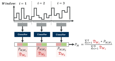
Figure 1. Proposed Methodology: The decision for i-th window $P_{M,W_{i}}$ is enhanced by the Malicious Discriminative Score $\mathfrak{D}_{W_{i}}$. This score adjustment corrects mis-classifications of benign segments within a malware-labeled time-series, thereby improving the precision of malware detection.

Our empirical study leverages the HMD model dataset from Kumar et al. (Kumar et al., 2023), examining multivariate time-series data derived from SoC components using Dynamic Voltage and Frequency Scaling (DVFS) and SYSFS telemetry. We introduce the Malicious Discriminative Score (MDS) to evaluate the distinctivenes of segment behaviors, assigning higher scores to segment-behaviors uniquely observed in malware time-series. This score enhances the classifier’s output by amplifying the signal for distinct malware behavior and attenuating it for benign behavior, thus fine-tuning the prediction for each time segment. Illustrated in Figure 1, the prediction for each window ($P_{M,W_{i}}$) is adjusted by its corresponding MDS ($\mathfrak{D}_{W_{i}}$), and the overall prediction $P_{M}$ is computed as the weighted sum of these adjusted segment predictions. To calculate the MDS, we model first-order interactions between time-series channels using conditional histograms, learning complex behavioral patterns as compared to single channel analysis which treat each channel of the multivariate time-series independently. Our key contributions are:

• Introduction of MIL formulation for accurate representation of malware behavior in segmented time-series, to reduce False Positives in real-time HMDs.

• Proposal of MDS to support the MIL assumption, calculated using a novel statistical classifier by analyzing first-order interactions in multivariate time-series.

The rest of the paper is organized as follows. We provide a brief background in Section 2. Next, we explain our proposed framework in Section 3. We present our evaluation results and discussion in Section 4 and conclude in Section 5.

2. Background

2.1. HMD and Related Works

Demme et al. leveraged Hardware Performance Counters (HPCs) to detect a range of malicious activities (Demme et al., 2013). Subsequent research has focused on improving HMDs’ predictive capabilities (Khasawneh et al., 2020; Kumar et al., 2021) and reducing their performance overhead (Patel et al., 2017; Cronin and Yang, 2018; Ozsoy et al., 2015). Alternatives to HPCs, such as DVFS telemetry (Chawla et al., 2021), have also been explored for their system-wide behavior profiling across various SoC sub-devices, widening the scope of detectable attacks beyond those with prominent architectural side-channel effects (Kumar et al., 2023).

Efforts to address real-time detection challenges have been noted (Alam et al., 2019; Ozsoy et al., 2015; Khasawneh et al., 2020; Kuruvila et al., 2021; Cronin and Yang, 2018). Alam et al. used an anomaly detection approach based on reconstruction error for real-time detection, avoiding direct benign vs. malware classification and focusing on normal vs. anomalous behavior (Alam et al., 2019). However, the variability in defining ”normal” often leads to high false positives in anomaly detection. In contrast, the benign vs. malware classification paradigm persists (Ozsoy et al., 2015; Khasawneh et al., 2020; Kuruvila et al., 2021; Cronin and Yang, 2018). While a broad classification of the entire time-series as malware might be justifiable (given the presence of malicious code) as done in prior works (Demme et al., 2013), using the parent labels for the windows is inadequate as it mislabels benign behavior. Kuruvila et al. suggested using ensemble of classifiers operating on extended window lengths to reduce false positives (Kuruvila et al., 2021). However, increased window lengths delay early detection. Our method diverges by preserving the window length, enabling timely detection, and utilizing the uniqueness of malicious behavior to fine-tune the window predictions, reducing false positives.

2.2. Multiple Instance Learning Formulation and Its Implementation Challenges

The crux of MIL is distinguishing between ‘bags’—the entire time-series—and ‘instances’—the segmented windows within (Foulds and Frank, 2010). Our MIL assumption assumes that a bag acquires a malware label if any instance within exhibits malware characteristics, reflecting the locality in malicious behavior within a malware time-series. This deviates from the current assumption where all instances inherit the bag’s label (Ozsoy et al., 2015; Khasawneh et al., 2020; Kuruvila et al., 2021; Cronin and Yang, 2018). A primary challenge in MIL is the absence of segment-level labels, which would otherwise require intensive forensic analysis to assign accurately. Such granularity in labeling is both impractical and unscalable due to the resources it demands. We address this by adopting a data-driven approach to learn what constitutes a malicious segment within a time-series: it must be unique to malware-labeled bags within the training dataset, and exhibit significant deviation from its benign counterpart. This operational definition aims to isolate high-discriminatory malicious segments, enhancing the fidelity of malware detection.

Table 1. Hardware telemetry channels in the dataset (Kumar et al., 2023)

Telemetry Class	Channel #	Description
DVFS	1	GPU controller
	2	CPU controller: lower cluster
	3	CPU controller: higher cluster
	4	CPU bus bandwidth controller
	5	GPU bus bandwidth controller
	6	GPU bus bandwidth controller
	7	Latency controller L3 cache: lower cluster
	8	Latency controller L3 cache: higher cluster
	9	Last level cache controller
	10	Memory latency controller: lower cluster
	11	Memory latency controller: higher cluster
SYSFS	12	Network: received bytes
	13	Network: transmitted bytes
	14	Device current
	15	Device voltage

2.3. Dataset Information

We use the dataset from Kumar et al. (Kumar et al., 2023), consisting of telemetry data focusing on DVFS and SYSFS states in an SoC. The telemetry is collected on a commodity Android smartphone. The DVFS states, crucial for power management, reflect the workload-induced activity in CPU, GPU, buses, caches, memory, and network interfaces (see Table 1). The dataset contains 1033 malware and 723 benign Android applications sourced from AndroZoo between December 2019 and June 2021. The malware apps span 54 families, verified by the ESET-NOD32 AV engine on VirusTotal. Each app’s hardware telemetry signature, collected over eight iterations, results in 2,120 signatures for malicious and 2,143 for benign apps, with each signature being a multivariate-time-series capturing 40 seconds of application execution. We employ a 70-30 train-test split with the test set comprising applications absent from the training set.

2.4. Threat Model

RT-HMD assumes attackers can deploy malware to manipulate application-level activities without root access, similar to (Kumar et al., 2023). Designed for multi-core mobile devices, RT-HMD operates under the premise that users engage with a limited number of foreground applications (1-2) simultaneously. This assumption is due to the reliance on system-wide telemetry channels (Table 1), capturing data from all device processes. RT-HMD’s training necessitates malware behavior profiling within a controlled sandbox environment. Consequently, any sandbox evasion techniques could compromise this profiling process, impacting the quality of training data and, ultimately, malware detection effectiveness in real-world scenarios. Additionally, RT-HMD is vulnerable to collusion-based attacks, where attacker-controlled threads could interfere with system-wide telemetry, potentially skewing detection capabilities.

Figure 2. Overview of the Malicious Discriminative Score (MDS): (a) [Top] Malware time-series with annotated benign and malicious segments [Bottom] Segmented benign time-series; (b) hyperplane under strong supervision assumption (current) and hyperplane under MIL assumption (proposed); (c) MDS functionality explained.

3. Proposed Framework

3.1. Overview

The key problem in malware detection using segmented time-series data is the presence of benign segments in both malware and benign-labelled series, leading to conflicting labels and noisy supervision during model training. Figure 2.a illustrates this, depicting a malware (1) and a benign (0) time-series, each segmented and labeled. Notably, we can observe benign segments within the malware time-series. These segments receive conflicting labels, blurring the classification boundary. In Figure 2.b, we visualize the classifier’s latent space, partitioned into three regions: segments unique to malware (lower left), common benign segments (middle), and segments unique to benign time-series (upper right). The overlap of benign segments in both malware and benign time-series complicates the classifier’s decision-making, resulting in high false positives.

To address this, we introduce the Malicious Discriminative Score (MDS). MDS evaluates the distinctiveness of segment behaviors, assigning higher scores to behaviors uniquely observed in malware time-series. In Figure 2.c, the effectiveness of MDS is demonstrated. The model generates a prediction, $P_{M,W_{i}}$, for a test segment, and MDS ($\mathfrak{D}_{W_{i}}$) is independently computed based on the observed segment behavior. The MDS is low for malware-labelled benign segments (first row) and high for unique malicious segments (second row). By multiplying the MDS with the model’s prediction, it either amplifies or attenuates the segment-prediction, enhancing confidence for uniquely malicious behaviors and reducing it for mis-labelled benign behaviors. Effectively, this process adjusts the classifier’s hyperplane, as shown in Figure 2.b, correcting false positives arising from the mis-labelled benign segments.

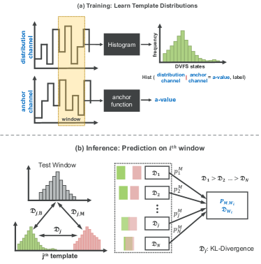
Figure 3. Illustrates the Training and Inference steps of the Interaction-based Statistical Classifier

Algorithm 1 Training and Inference Approach

0:  $X$: Multivariate time-series with $C$ channels  $B$: Number of histogram bins $W$: Window size $AF$: Anchor function

0:  $\theta$: Template distributions for training $P_{M}$: Malware probability for inference

1:  Training Phase:

2:  for $c_{1}=1$ to $C-1$ do

3:     for $c_{2}=c_{1}+1$ to $C$ do

4:        Select channel $c_{1}$ as distribution-channel

5:        Select channel $c_{2}$ as anchor-channel

6:        for non-overlapping windows $w\in W$ do

7:           $h_{w}\leftarrow$ Histogram$(X_{c_{1},w},B)$ {Create histogram}

8:           $a_{w}\leftarrow AF(X_{c_{2},w})$ {Determine anchor value}

9:           $\theta_{c_{1},c_{2}}\leftarrow\theta_{c_{1},c_{2}}\cup{(h_{w},a_{w})}$ {Store template}

10:        end for

11:     end for

12:  end for

13:  Inference Phase:

14:  for windows $w\in W$ do

15:     $\hat{h}_{w},\hat{a}_{w}\leftarrow$ Histogram & Anchor$(X_{w})$ {Generate for distr. and anchor-channels}

16:     for $c_{1}=1$ to $C-1$ do

17:        for $c_{2}=c_{1}+1$ to $C$ do

18:           $\Phi_{w,B}^{c_{1},c_{2}}\leftarrow KL(\hat{h}_{w},\theta_{c_{1},c_{2}}^{B})$ {Benign KL divergence}

19:           $\Phi_{w,M}^{c_{1},c_{2}}\leftarrow KL(\hat{h}_{w},\theta_{c_{1},c_{2}}^{M})$ {Malware KL divergence}

20:           $P^{c_{1},c_{2}}_{M,w}\leftarrow\text{softmax}({\Phi_{w,B}^{c_{1},c_{2}},\Phi_{w,M}^{c_{1},c_{2}}})$ {Malware probability}

21:        end for

22:     end for

23:     for $(c_{1},c_{2})\in C\times C$ do

24:        $\mathfrak{D}_{w}^{c_{1},c_{2}}\leftarrow KL(\theta_{c_{1},c_{2}}^{B},\theta_{c_{1},c_{2}}^{M})$ {MDS}

25:     end for

26:     $P_{M,w}\leftarrow\sum_{c_{1},c_{2}}P_{M,w}^{c_{1},c_{2}}\mathfrak{D}_{w}^{c_{1},c_{2}}/\sum_{c_{1},c_{2}}\mathfrak{D}_{w}^{c_{1},c_{2}}$

27:     $\mathfrak{D}_{w}\leftarrow\sum_{c_{1},c_{2}}\mathfrak{D}_{w}^{c_{1},c_{2}}$

28:  end for

3.2. Training: Learning Template Distributions

The training approach, illustrated in Figure 3.a and summarized in Algorithm-1 Training Phase, focuses on creating template conditional distributions using empirical histograms. This process involves moving a non-overlapping sliding window across the multi-variate time-series. Within each window, a pair of channels is selected: one as the distribution-channel and the other as the anchor-channel. For the distribution-channel, a histogram based on the observed DVFS states is constructed, and for the anchor-channel, a representative anchor-value (a-value) is calculated using a predefined anchor function. Combined with the labels that distinguish between benign and malicious data sources, this forms a conditional distribution, expressed as:

(1) $$\text{P}_{\text{template}}\left[\begin{subarray}{c}\text{distribution}\\ \text{channel}\end{subarray}\bigg{|}\left(\begin{subarray}{c}\text{anchor}\\ \text{channel}\end{subarray}=\text{a-value},\text{label}\right)\right]$$

Generating the Template Conditional Distributions. As the sliding window traverses each segment of the time-series, it systematically captures key parameters of the conditional distribution such as the distribution-channel, anchor-channel, anchor-value, and label, which are used as unique keys to retrieve and update the corresponding template histogram with new values (using add operation). This method, applied across all multivariate time-series in the training dataset creates a set of template conditional distributions, through which we have learned the likelihood of observing distributions in one channel, conditioned on a representative value in another channel given the application class (malware or benign). The MDS is defined as the Kullback-Leibler (KL) Divergence between template conditional distributions sharing the same distribution-channel, anchor-channel, and anchor-value, but differing in labels: one benign, one malicious. Intuitively, MDS measures the uniqueness of interactions, with higher values signaling exclusive malware behavior and lower ones indicating segment-behavior common to both benign and malware time-series.

There are three key parameters used in generating the conditional distributions: the number of histogram bins ($B$), the window size ($W$), and the anchor function ($AF$). A grid search was performed over $B$ and $W$ to identify the optimal configuration which maximizes the MDS recorded over all the template distributions. The $AF$ is used to calculate the anchor-value which is bucketized to the nearest bin to simplify the tracking of template histograms. Number of tracked template histograms: Given $N$ channels in a multivariate time-series from an application sample, there are $N$ possible distribution-channel values and $N-1$ anchor-channel values. Each anchor-value can assume $B$ values, and distributions are tracked separately for benign and malicious labels. Thus, the overall number of template distributions monitored during training is $N*N-1*B*2$.

3.3. Inference Methodology

The inference approach is illustrated in Figure 3.b and summarized in the Inference Phase of Algorithm 1. It mirrors the training phase by generating inference conditional distribution for each pairwise channel. The recorded distribution-channel, anchor-channel, anchor-value parameters are used to fetch the corresponding benign and malware template distributions ($j^{th}$). The objective is to determine if the inference distribution resembles malware or benign behavior recorded by the template distributions learned during training. This is determined using the following KL-divergence scores: (1) KL divergence between the benign template distribution and the inference distribution ($\Phi_{j,B}$), assessing similarity to the benign behavior; (2) KL divergence between the malware template distribution and the inference distribution ($\Phi_{j,M}$), evaluating similarity to the malware behavior. A softmax operation, as shown in Equation 2, calculates the malware probability:

(2) $$P_{j,M}=\frac{e^{-\Phi_{j,M}}}{e^{-\Phi_{j,M}}+e^{-\Phi_{j,B}}}$$

This operation offers a probabilistic measure of an interaction being malicious. For each pairwise interaction within the inference window ($N\times N-1$ possible interactions), a softmax probability is calculated, reflecting the interaction’s similarity to malware behavior. The final prediction probability for the i-th window, $P_{M,W_{i}}$, is obtained by averaging $P_{j,M}$ for all $j$ in $N\times(N-1)$. For a uniquely malicious segment, $\Phi_{j,M}>\Phi_{j,B}$, so that $P_{j,M}>0.5$. However, if benign and malware interactions are similar, due to ambiguous labeling (Ozsoy et al., 2015; Khasawneh et al., 2020; Kuruvila et al., 2021; Cronin and Yang, 2018), $\Phi_{j,B}\approx\Phi_{j,M}$ , resulting in $P_{j,M}$ and consequently $P_{M,W_{i}}\approx 0.5$. This ambiguity indicates classifier confusion due to conflicting labels, resulting in erroneous predictions.

MDS-weighted decisions. To address this, we use the MDS to refine our prediction process. Rather than a simple average, $P_{M,W_{i}}$ is computed as a weighted average using the MDS values ($\mathfrak{D}_{j}$) of the corresponding template distributions, as shown in Equation 3. This modification ensures that if benign and malware interactions are similar, resulting in a lower $\mathfrak{D}_{j}$, the prediction probability is attenuated so that $P_{j,M}<<0.5$. The total MDS for the i-th window ($\mathfrak{D}_{W_{i}}$) is the sum of MDS values for all participating conditional distributions, quantifying the overall MDS within the window, as shown in Equation 4.

(3) $$P_{M,W_{i}}=\frac{\sum_{j=1}^{N\times(N-1)}\mathfrak{D}_{j}\times P_{j,M}}{\sum_{j=1}^{N\times(N-1)}\mathfrak{D}_{j}}$$

(4) $$\mathfrak{D}_{W_{i}}=\sum_{i=1}^{N\times(N-1)}\mathfrak{D}_{j}$$

This approach allows $P_{M,W_{i}}$ to factor in the similarity of benign and malware interactions, thus refining the quality of the final prediction for each window.

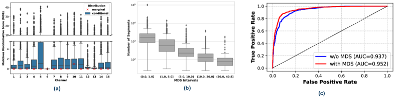
Figure 4. (a) Boxplot showing MDS of the template distributions for two modalities of information: interaction (conditional distributions) and channels of time-series treated independently (marginal distribution) for different distribution-channels. Marginals do not capture the high MDS behaviors between benign and malware; (b) Boxplot showing the frequency of occurrence of segments (total segments: 101863, segment-length$\approx$1s) stratified by MDS in the training dataset (y-axis is logarithmic). High MDS interactions are less frequent; (c) Increase in AUC upon using MDS weighted decision.

4. Evaluation results

4.1. Analyzing Segment Behavior

Distinguishability of Interactions. We examine distinguishability of multi-variate interactions within a time segment, assessed via the MDS of the template distributions. Figure 4.a shows the MDS obtained from template conditional distributions. We observe a wide variance in MDS values indicating that the template distributions are learning both unique and common behaviors between the malware and benign time-series segments. Channels with limited DVFS states, such as channel-5, yield lower MDS due to insufficient information for capturing interactions. The marginal template distributions which treats the channels independently as shown in Equation 5, are depicted with markers and consistently show lower MDS values. This underlines the necessity of leveraging conditional distributions to extract a richer set of discriminative features, highlighting the importance of inter-channel interactions over single channel analysis in a multi-variate time-series.

(5) $$\text{P}_{\text{template}}\left[\begin{subarray}{c}\text{distribution}\\ \text{channel}\end{subarray}\bigg{|}\text{label}\right]$$

Frequency of High MDS Segments in time-series. Next, we aim to quantify the occurrence of high MDS segments, which are indicative of distinct malware interactions, against the backdrop of our hypothesis that a malware time-series comprises both benign and malicious segments. Figure 4.b shows the number of segments (in the training dataset) that contribute to template distributions across various MDS intervals. The y-axis, on a logarithmic scale, represents the count of segments, while the x-axis shows MDS intervals. The plot reveals a predominance of lower MDS segments, suggesting that common interactions arising from malware-labelled benign segments are frequently encountered, which substantiates our hypothesis. Conversely, segments with high MDS that reflect unique behaviors specific to malware, are rarer. This observation confirms our intuition that labeling segments solely based on the time-series they belong to—as current methods do—results in mislabeling, given the frequent commonality between segments observed in benign and malware labeled time-series.

4.2. Impact on Classification Performance

Table 2. Precision and Recall for different anchor functions

Anchor Function	Precision		Recall
	w/o MDS	with MDS	w/o MDS	with MDS
max	0.86	0.89	0.89	0.89
mean	0.80	0.85	0.85	0.89
median	0.84	0.88	0.88	0.90
min	0.83	0.87	0.89	0.89
mode	0.85	0.90	0.89	0.89

Classifier Performance with MDS Weighting. Our evaluation investigates how MDS weighting influences classifier metrics, such as precision and recall, compared to baseline methods that average predictions without weighting. Due to the absence of ground truth for individual segments, we assess performance based on the entire time-series. The overall time-series prediction with MDS weighting is computed as:

(6) $$P_{M}=\frac{\sum_{i=1}^{S}\mathfrak{D}_{W_{i}}\times P_{M,W_{i}}}{\sum_{i=1}^{S}\mathfrak{D}_{W_{i}}}$$

We compare the MDS-weighted decision to a baseline that aggregates predictions without MDS weighting, reflecting current practices where benign segments in malware time-series are inaccurately labeled (Ozsoy et al., 2015; Khasawneh et al., 2020; Kuruvila et al., 2021; Cronin and Yang, 2018). We report our findings in Figure 4.c and Table 2. The ROC curve in Figure 4.c, with the mode as the anchor function, shows an improvement in AUC score when incorporating MDS weighted decision. Notably, for a given True Positive Rate (TPR), the MDS-weighted classifier demonstrates a reduced False Positive Rate (FPR), signifying a refined specificity. Table 2 further reveals that across different anchor functions, MDS weighting consistently enhances precision without compromising—and occasionally improving—recall. This performance improvement aligns with our hypothesis that MDS weighting mitigates the impact of incorrectly labelled benign segments, thereby improving precision. It’s important to note that while Kumar et al.’s dataset is balanced, in real-world scenarios—where benign instances vastly outnumber malicious ones—the observed precision improvement serves as a conservative estimate, as precision is particularly sensitive to the prevalence of benign samples which have a higher base rate in malware detection (Arp et al., 2022).

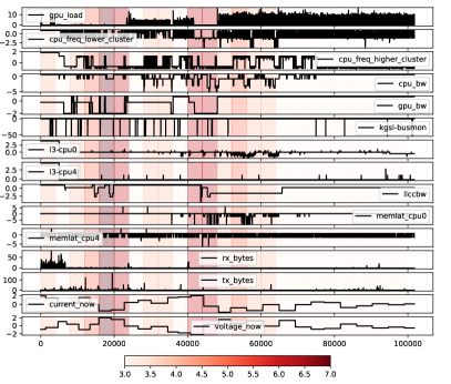
Figure 5. An MDS-based saliency heatmap highlighting localized malicious behavior within the hardware telemetry (multivariate time-series). Each channel of the time-series corresponds to the channels outlined in Table 1.

Enhanced Interpretability through MDS. Our model introduces a refined layer of interpretability by utilizing the product of $\mathfrak{D}_{W_{i}}$ and $P_{M,W_{i}}$ as attention weights, as depicted in Figure 5. Unlike traditional interpretability mechanisms that generate saliency maps without explaining the underlying rationale, the MDS-based saliency map assigns a definitive meaning to these weights, suggesting that the classifier detects behavior with a high discriminative capability. The saliency map in Figure 5 illustrates the classifier’s capability to localize malicious segments, supporting our hypothesis that not all segments of a malware time-series demonstrate distinctively malicious behavior.

5. Conclusion and Future Work

In conclusion, our research addresses a critical gap in HMDs by introducing a MIL framework that captures the episodic nature of malware within segmented time-series data, mitigating the label misrepresentation and subsequent false positives. Leveraging the MDS, we enhance HMD performance by distinguishing between benign and malicious segment behaviors, enhancing the precision and interpretability of threat detection. Our empirical results, demonstrated using a novel statistical classifier, confirm the efficacy of the MIL formulation in the development of robust real-time malware detection solutions. While this study concentrates on statistical classification methods applied to DVFS-based time-series, future works aim to extend MDS computation to ML algorithms and examine its viability in Hardware Performance Counter contexts, broadening the scope and applicability of the proposed solution.

References

- (1)
- int ([n. d.]) [n. d.]. Detect Ransomware and Other Advanced Threats with Intel Threat Detection Technology. https://www.intel.com/content/dam/www/public/us/en/documents/solution-briefs/threat-detection-technology-solution-brief.pdf.
- mic ([n. d.]) [n. d.]. Microsoft Defender for Endpoint. https://docs.microsoft.com/en-us/microsoft-365/security/defender-endpoint/microsoft-defender-endpoint?view=o365-worldwide.
- noa ([n. d.]) [n. d.]. Qualcomm Mobile Security. https://www.qualcomm.com/products/features/mobile-security/snapdragon-malware-protection.
- fir ([n. d.]) [n. d.]. Threat Intelligence Reports. https://www.fireeye.com/current-threats/threat-intelligence-reports.html.
- Alahmadi et al. (2022) Bushra A. Alahmadi, Louise Axon, and Ivan Martinovic. 2022. 99% False Positives: A Qualitative Study of SOC Analysts’ Perspectives on Security Alarms. In 31st USENIX Security Symposium (USENIX Security 22). USENIX Association, Boston, MA, 2783–2800. https://www.usenix.org/conference/usenixsecurity22/presentation/alahmadi
- Alam et al. (2019) Manaar Alam, Sarani Bhattacharya, Swastika Dutta, Sayan Sinha, Debdeep Mukhopadhyay, and Anupam Chattopadhyay. 2019. RATAFIA: Ransomware Analysis using Time And Frequency Informed Autoencoders. In 2019 IEEE International Symposium on Hardware Oriented Security and Trust (HOST). 218–227. https://doi.org/10.1109/HST.2019.8740837
- Arp et al. (2022) Daniel Arp, Erwin Quiring, Feargus Pendlebury, Alexander Warnecke, Fabio Pierazzi, Christian Wressnegger, Lorenzo Cavallaro, and Konrad Rieck. 2022. Dos and Don’ts of Machine Learning in Computer Security. In 31st USENIX Security Symposium (USENIX Security 22). USENIX Association, Boston, MA, 3971–3988. https://www.usenix.org/conference/usenixsecurity22/presentation/arp
- Chawla et al. (2021) Nikhil Chawla, Arvind Singh, Harshit Kumar, Monodeep Kar, and Saibal Mukhopadhyay. 2021. Securing IoT Devices Using Dynamic Power Management: Machine Learning Approach. IEEE Internet of Things Journal 8, 22 (2021), 16379–16394. https://doi.org/10.1109/JIOT.2020.3021594
- Cronin and Yang (2018) Patrick Cronin and Chengmo Yang. 2018. Lowering the barrier to online malware detection through low frequency sampling of HPCs. In 2018 IEEE International Symposium on Hardware Oriented Security and Trust (HOST). 177–180. https://doi.org/10.1109/HST.2018.8383910
- Demme et al. (2013) John Demme, Matthew Maycock, Jared Schmitz, Adrian Tang, Adam Waksman, Simha Sethumadhavan, and Salvatore Stolfo. 2013. On the Feasibility of Online Malware Detection with Performance Counters. In Proceedings of the 40th Annual International Symposium on Computer Architecture (Tel-Aviv, Israel) (ISCA ’13). Association for Computing Machinery, New York, NY, USA, 559–570. https://doi.org/10.1145/2485922.2485970
- Foulds and Frank (2010) James Foulds and Eibe Frank. 2010. A review of multi-instance learning assumptions. The Knowledge Engineering Review 25, 1 (2010), 1–25. https://doi.org/10.1017/S026988890999035X
- Kazdagli et al. (2016) Mikhail Kazdagli, Vijay Janapa Reddi, and Mohit Tiwari. 2016. Quantifying and improving the efficiency of hardware-based mobile malware detectors. In 2016 49th Annual IEEE/ACM International Symposium on Microarchitecture (MICRO). 1–13. https://doi.org/10.1109/MICRO.2016.7783740
- Khasawneh et al. (2020) Khaled N. Khasawneh, Meltem Ozsoy, Caleb Donovick, Nael Abu-Ghazaleh, and Dmitry Ponomarev. 2020. EnsembleHMD: Accurate Hardware Malware Detectors with Specialized Ensemble Classifiers. IEEE Transactions on Dependable and Secure Computing 17, 3 (2020), 620–633. https://doi.org/10.1109/TDSC.2018.2801858
- Kumar et al. (2023) Harshit Kumar, Biswadeep Chakraborty, Sudarshan Sharma, and Saibal Mukhopadhyay. 2023. XMD: An Expansive Hardware-Telemetry-Based Mobile Malware Detector for Endpoint Detection. IEEE Transactions on Information Forensics and Security 18 (2023), 5906–5919. https://doi.org/10.1109/TIFS.2023.3318969
- Kumar et al. (2021) Harshit Kumar, Nikhil Chawla, and Saibal Mukhopadhyay. 2021. Towards Improving the Trustworthiness of Hardware based Malware Detector using Online Uncertainty Estimation. In 2021 58th ACM/IEEE Design Automation Conference (DAC). 961–966. https://doi.org/10.1109/DAC18074.2021.9586288
- Kuruvila et al. (2021) Abraham Peedikayil Kuruvila, Sayar Karmakar, and Kanad Basu. 2021. Time Series-Based Malware Detection Using Hardware Performance Counters. In 2021 IEEE International Symposium on Hardware Oriented Security and Trust (HOST). 102–112. https://doi.org/10.1109/HOST49136.2021.9702291
- Küchler et al. (2021) Alexander Küchler, Alessandro Mantovani, Yufei Han, Leyla Bilge, and Davide Balzarotti. 2021. Does Every Second Count? Time-based Evolution of Malware Behavior in Sandboxes. https://doi.org/10.14722/ndss.2021.24475
- Ozsoy et al. (2015) Meltem Ozsoy, Caleb Donovick, Iakov Gorelik, Nael Abu-Ghazaleh, and Dmitry Ponomarev. 2015. Malware-aware processors: A framework for efficient online malware detection. In 2015 IEEE 21st International Symposium on High Performance Computer Architecture (HPCA). 651–661. https://doi.org/10.1109/HPCA.2015.7056070
- Patel et al. (2017) Nisarg Patel, Avesta Sasan, and Houman Homayoun. 2017. Analyzing hardware based malware detectors. In 2017 54th ACM/EDAC/IEEE Design Automation Conference (DAC). 1–6. https://doi.org/10.1145/3061639.3062202