Spatial curvature with the Alcock-Paczyński effect

Abstract

We propose a methodology to measure the cosmological spatial curvature by employing the deviation from statistical isotropy due to the Alcock-Paczyński effect of large scale galaxy clustering. This approach has a higher degree of model independence than most other proposed methods, being independent of calibration of standard candles, rulers, or clocks, of the power spectrum shape (and thus also of the pre-recombination physics), of the galaxy bias, of the theory of gravity, of the dark energy model and of the background cosmology in general. We find that a combined DESI-Euclid galaxy survey can achieve $\Delta\Omega_{k0}=0.057$ at 1$\sigma$ C.L. in the redshift range $z<2$ by combining power-spectrum and bispectrum measurements.

I Introduction

The spatial curvature $\Omega_{k0}$ has been one of the most investigated cosmological parameters over the last decades. It is a standard degree of freedom of the Friedman-Lemaître-Robertson-Walker metric, with a very important role in our understanding of the universe. The possibility of a non-flat universe thus continues to captivate both researchers and laymen.

The first strong observational constraints on flatness came from the measurements of the first peak of the Cosmic Microwave Background (CMB) angular power spectrum [1]. Since then, high-resolution maps of the CMB have continued to tighten these constraints and the current best one comes from the Planck satellite. There is, however, a strong debate on which are the current most reliable measurements. The combination of temperature, polarization and lensing yields $\Omega_{k0}=-0.0106\pm 0.0065$ [2], consistent with flatness. But the CMB lensing itself is too large to fit the standard $\Lambda$CDM model [3, 4]. Dropping lensing, one gets $-0.095<\Omega_{k0}<-0.007$ at 99% CL [5], favoring a closed universe. This disagreement highlights the fact that CMB measurements are always performed within a cosmological paradigm which requires assuming a specific model for both the early and late universes.

Curvature can also be measured through its effects on the late-time universe. In particular, it affects measurements of the luminosity ($D_{L}$) and angular diameter ($D_{A}$) distances, of the expansion rate ($H(z)$) and of both weak and strong lensing. A large number of works analyzed combinations of these observables to constrain curvature independently from the CMB. Several of these made use of the so-called cosmic chronometers (CC) to infer $H(z)$ and constrained $\Omega_{k0}$ by combining $H(z)$ with supernova distances (SN) [6, 7, 8, 9, 10, 11, 12], with BAO [13, 14, 10, 12], or with lensing [15]. The obtained uncertainties on $\Omega_{k0}$ are around $\sim 0.1-0.2$. However, CC are based on modelling passively evolving galaxies, and their accuracy level is still under debate [16]. Without CC, constraints on $\Omega_{k0}$ were also obtained with precision $\sim 0.5-0.9$ combining supernova distances and lensing [17]. A promising avenue to avoid CC relies on measurements of the large-scale structure (LSS) alone, since radial and transversal correlations allow measurements of both $D_{A}(z)$ and $H(z)$. The recent DESI 2024 results using BAO alone obtained $\Omega_{k0}=0.065^{+0.068}_{-0.078}$ ($0.087^{+0.100}_{-0.085}$) assuming the $\Lambda$CDM (o$w_{0}w_{a}$CDM) model [18].

Forecasts on $\Omega_{k0}$ have also been performed using weak-lensing from Euclid or LSST [19]; intensity mapping [20]; supernovae and BAO [11]; standard sirens [21, 22] and the clustering of standard candles [23, 22].

One important recent concern in the field has been to push for model-independent measurements. Non-parametric fits have been employed to mitigate late-time modelling using Gaussian Processes [7, 24, 11, 12], polynomial fits [9] or smoothing techniques [25]. Another option is to use directly the measurements of $D_{A}$ and $H$ in different redshift bins [6, 26]. Here we follow the latter approach.

This late-time model-independence has the advantage of being robust with respect to uncertainties related to dark energy, which is important since there are hints of a tension with late-universe data (e.g. [27, 18]). We remark that model-independence however can also be extended to the early universe, as we will discuss below, which makes results also robust against non-standard early universe physics. In fact, the current Hubble tension has sparked interest in more exotic early universe scenarios as a possible explanation [28]. Extending model-independence to the early universe means we do not have to assume that $P(k)$ has the $\Lambda$CDM shape, or is parametrized by a restricted set of parameters, for instance the Alcock-Paczyński (AP) parameters $\alpha_{\parallel},\alpha_{\perp}$, plus the growth rate $f$ and the normalization $\sigma_{8}$ as in, e.g., [29] where, moreover, the non-linear corrections were evaluated only for the $\Lambda$CDM model. Thus, to the best of our knowledge, no work so far has investigated the possibility of measuring the spatial curvature in the same model-independent way that we propose in this paper.

In this work we employ the FreePower method [30, 31, 32]. FreePower extracts cosmological information in a purely geometrical way through the AP effect by binning the spectra in $k$-wavebands. The AP effect depends only on the dimensionless expansion rate $E$ and the dimensionless comoving angular diameter distance $L_{A}$

$$E(z)\equiv H(z)/H_{0}\,,\quad L_{A}(z)\equiv H_{0}D_{A}(z)\,.$$ (1)

Instead of choosing a particular cosmological model, the method leaves free to vary, in each redshift bin, the functions $f$, $E$ and $L_{A}$ together with all necessary nuisance parameters. We take as data the one-loop power spectrum and tree-level bispectrum of galaxy clustering. Our strategy is to use only the AP effect to constrain both $E$ and $L_{A}$ while ensuring that the clustering correlators are written down in the most model-independent way and all relevant parameters are marginalized over. We adopt for the non-linear correlators the general expressions derived in [33], which is based on general considerations of symmetry rather than on specific models. Our basic parameters are then 25 values of the linear $P(k_{i})$ in the $k$ interval $0.01-0.25\,h/$Mpc, plus, for each redshift bin, $f$, $E$ and $L_{A}$, seven bias and bootstrap parameters, a smoothing velocity dispersion and a counterterm parameter, and finally three shot noises. In total, we have 15 parameters for each redshift bin plus 25 $k$-band parameters. We adopt two cut-off schemes: a more “aggressive” one, which is our default scheme, in which we take $k_{\rm max}=0.25\,h/$Mpc for the power spectrum and $k_{\rm max}^{\rm B}=0.1\,h/$Mpc for the bispectrum; and a “conservative” one, in which the two cut-offs are $0.20\,h/$Mpc and $0.08\,h/$Mpc, respectively. We assume that $f$ does not depend on $k$ in the interval here considered. This is not a fundamental limitation, as we have shown in [31], but it is a safe approximation in many models (e.g., massive neutrinos induce a variation of $f$ with $k$ of less than 1% in the viable range, see e.g. [34]). More details in Ref. [32].

	$z$	$V$	$10^{3}\,n_{g}$	$b_{1}$
		​​[Gpc$/h]^{3}\!\!$	$[h/{\rm Mpc}]^{3}$
	0.1	0.263	118.	1.41
	0.3	1.53	11.9	1.57
DESI	0.5	3.33	1.14	1.74
	0.7	5.15	1.07	1.15
	0.9	7.22	1.54	1.26
	1.1	8.61	0.891	1.34
	1.3	9.66	0.521	1.42
Euclid	1.5	10.4	0.274	1.5
	1.7	11.	0.152	1.58
	1.9	11.3	0.0899	1.66

Table 1: Our forecast specifications and fiducials, based on DESI and Euclid forecasts for the full surveys. We use DESI BGS for $z<0.6$, DESI ELG for $0.6<z<0.8$ and Euclid ELG for $z>0.8$. For $z<0.6$ we take values for the bias parameters from the low-z BOSS results [35], while for $z>0.6$ we use the models in [36].

Our approach addresses therefore both the issue of improving accuracy (being more model-independent than other approaches) and improving precision (employing the information in the one-loop spectrum and in the bispectrum). Another crucial advantage of the FreePower approach is that we can derive constraints directly on the dimensionless variables $E$ and $L_{A}$, and thus directly on $\Omega_{k0}$. This is in contrast with using the popular combination CC and SN or standard sirens, which constrains only the quantity $\Omega_{k0}$$H_{0}^{2}$, and thus requires either an extra probe to constrain $H_{0}$ or an extrapolation of the $H(z)$ data to $z\rightarrow 0$ to break the degeneracy.

II Spatial curvature constraints

We applied the FreePower method to produce Fisher matrix forecasts for a joint DESI and Euclid dataset. The DESI survey [37, 38] is a ground telescope which will produce a spectroscopic map covering 14000 deg² of the sky, covering the range $z=(0-1.6)$ with a combination of BGS, LRG and ELG galaxies [39]. The Euclid survey is a space telescope, launched in 2023, that will map 15000 deg² of the sky [40], covering the range $z=[0.8-2.0]$. We adopted redshift bins of width $\Delta z=0.2$ centered on the redshifts listed in the tables, and assume negligible cross-bin correlations. We used DESI specifications (only for BGS and low-redshift ELG in order to be conservative) for the bins with $z\leq 0.8$ and Euclid for $0.8\leq z\leq 2.0$. The main details of the surveys and the fiducial parameters are displayed in Table 1. This is similar to what was considered in [41]; the main difference with respect to [32] is the inclusion of the low-$z$ DESI bins.

As mentioned above, the AP effect distorts the wavenumber $k$ and the cosine angle $\mu$ in a way that depends only on $h\equiv E/E_{r}$ and $l\equiv L_{A}/L_{A,r}$, where the subscript $r$ refers to the (arbitrary) reference cosmological value adopted to convert distances and angles into $k,\mu$, such that $\mu=\mu_{r}h/\alpha$ and $k=\alpha k_{r}$, where [42, 43, 44]

$$\alpha\,=\,l^{-1}\sqrt{\mu_{r}^{2}(h^{2}l^{2}-1)+1}\,.$$ (2)

Once we marginalize over all the other parameters, we see that we can measure $h(z),l(z)$ down to 2–3% in several redshift bins in the aggressive case, as we show in Table 2. The marginalized Fisher matrix for $h,l$ is the main input for the next section.

$z$	$\Delta f/f$	$\Delta h/h$	$\Delta l/l$
0.1	0.072	0.038	0.024
0.3	0.052	0.023	0.015
0.5	0.044	0.019	0.013
0.7	0.034	0.022	0.018
0.9	0.031	0.019	0.016
1.1	0.03	0.018	0.015
1.3	0.032	0.019	0.015
1.5	0.039	0.021	0.017
1.7	0.049	0.025	0.02
1.9	0.063	0.031	0.026

Table 2: Fully marginalized relative error forecast for all redshift bins, (see [32] for a full description). Here and in then rest of this work we report 1$\sigma$ uncertainties.

The spatial curvature is related to $E(z)=H(z)/H_{0}$ and to the dimensionless comoving angular diameter distance $L_{A}(z)$ by a relation that in our $h,l$ variables reads

$$\Omega_{k0}=\frac{\big{(}h(\partial_{z}l)E_{r}L_{A,r}+hl\big{)}^{2}-1}{l^{2}L_{A,r}^{2}}\,,$$ (3)

where $\partial_{z}$ means derivative with respect to $z$. Notice that in terms of $E(z)$ and $L_{A}(z)$, $\Omega_{k0}$ is independent of $H_{0}$, as we discussed previously. Also, the expression above is valid for both open and closed curvature. Therefore, once we measure $E,L_{A}$, we can also measure $\Omega_{k0}$.

We need then to propagate the constraints on $h,l$ from each bin, including their correlation, to $\Omega_{k0}$. Since $\Omega_{k0}$ depends in a non-linear way on the variables $h,l$, we choose to propagate the errors numerically. We generate $10^{5}$ random values of $h,l$ in $n_{B}$ redshift bins $i=1,...,n_{B}$ from a Gaussian multivariate distribution with means 1 in each bin and covariance given by the inverse of our marginalized Fisher matrix for $h,l$. Then we discretize Eq. (3)

$$\Omega_{k,i}=\frac{\left[h_{i}\frac{(l_{i+1}-l_{i-1})}{2\Delta z}E_{r}(z_{i})L_{A,r}(z_{i})+h_{i}l_{i}\right]^{2}-1}{l_{i}^{2}L_{A,r}(z_{i})^{2}}\,,$$ (4)

where $\Delta z$ is the bin size, and from every set of $h_{i},l_{i}$ with $i=2,..n_{B}-1$ we produce a value of $\Omega_{k,i}$. The $j-$th value corresponding to the $i$-th bins is denoted as $\Omega_{k,(i,j)}$. These values are correlated. Then we estimate the $(n_{B}-2)\times(n_{B}-2)$ covariance matrix of $\Omega_{k,(i,j)}$:

$$C_{\Omega_{k,(i,n)}}=\big{\langle}\Omega_{k,(i,j)}\Omega_{k,(n,m)}\big{\rangle}_{j,m}\,.$$ (5)

The errors on $\Omega_{k0}$ for each bin are in Table 3, while in Fig. 1 we show the distribution for some redshift bins. Since the distribution is well approximated by a Gaussian, we can safely interpret the errors in the table in the usual Gaussian way, i.e. as 68$\%$ confidence regions. The variance of $\Omega_{k0}$ is obtained by projecting the $(n_{B}-2)\times(n_{B}-2)$ Fisher matrix $F=C^{-1}_{\Omega_{k0}}$ onto a single $\Omega_{k0}$. The result is simply

$$\sigma^{2}_{\Omega_{k0}}=\bigg{(}\sum_{i,j}F_{ij}\bigg{)}^{-1}\,.$$ (6)

Finally, we obtain

$$\sigma_{\Omega_{k0}}=0.057$$ (7)

at 68$\%$ for the aggressive specifications, and $\sigma_{\Omega_{k0}}=0.075$ for the conservative ones. If only the power spectrum is employed, then we get 0.094. If one artificially takes the limit of infinite galaxy number density, then the cosmic-variance limited value of 0.033 can be reached. These results, and the comparison with $\Lambda$CDM, are in Table 4. Let us remark that these results are not prior-dominated, that is, the priors for each parameter have been chosen to be much wider than the final constraints.

$z$	FreePower	FreePower	$\Lambda$CDM
		CV limit	$+\Omega_{k0}$
0.3	0.769	0.735	0.250
0.5	0.365	0.325	0.140
0.7	0.244	0.207	0.110
0.9	0.240	0.198	0.097
1.1	0.205	0.161	0.090
1.3	0.218	0.143	0.089
1.5	0.263	0.134	0.095
1.7	0.351	0.129	0.110
​combined	0.0572	0.0335	0.033

Table 3: Forecast uncertainties on $\Omega_{k0}$ for each bin (and combined). We also show the constraints for the standard full-shape approach assuming $\Lambda$CDM.

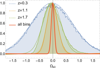
Figure 1: Numerical distribution of $\Omega_{k0}$ for two redshift bins. The dashed curves are Gaussian fits. The continuous thicker red curve is the likelihood when combining all bins.

How do these numbers compare with other methods with some degree of model independence? Forecasts for Euclid data using the standard full-shape approach, which assumes a parametrized shape of $P(k)$, and assuming linear theory was valid up to (an optimistic) $k_{\rm max}=0.20h$/Mpc were performed in [6]. They found $\sigma$($\Omega_{k0}$) around $0.1-0.2$ in 13 redshift bins, which if combined would result in $\sigma(\Omega_{k0})=0.033$. A forecast for Euclid + DESI was performed in [11] using the radial BAO scale combined with Nancy Roman SN, resulting in $\sigma(\Omega_{k0})=0.026$, but this assumes the BAO scale does not evolve. Forecasts for 21cm intensity mapping for HIRAX combining with the CMB distance scale were also performed in [20], resulting in $\sigma(\Omega_{k0})=0.0085$ for an agnostic binned $w(z)$ dark-energy model. Of course, assuming both an early and late-time model allows tighter constraints. For instance, the same HIRAX+CMB constraints shrink to $\sigma(\Omega_{k0})=0.0028$ assuming $w$CDM. Other methods also become very precise. Assuming the $\Lambda$CDM model, using the clustering of Einstein Telescope bright sirens and DESI BGS, $\sigma(\Omega_{k0})=0.018$ was forecast by [22], while combining upcoming CMB with Euclid BAO and weak-lensing could yield $\sigma(\Omega_{k0})=0.0018$ (degrading to $0.0088$ for the $w$CDM model) [19].

method	combined $\sigma_{\Omega_{k0}}$
FreePower P+B	$0.057$
FreePower conservative P+B	0.075
FreePower CV limit P+B	0.033
FreePower only P	0.094
$\Lambda$CDM full shape P+B	0.033
$\Lambda$CDM full shape only P	0.037
$\Lambda$CDM full shape P+B+CMB	0.0021

Table 4: Results combining all redshift bins. Note that CMB can only be added by considering a model for both early and late times. P stands for using the power spectrum alone while P+B adds also the bispectrum. CV limit denotes the cosmic variance limit, i.e. $n_{g}\rightarrow\infty$.

We emphasize that, in contrast with our approach, all these constraints have been obtained either assuming specific parametrizations, or the reliability, accuracy and correct calibration in general of standard candles and clocks. For CC in particular, this requires assuming the reliability and robustness of stellar population synthesis models, which form the basis of the method, and that all CC systematic effects can be kept under control.

Finally, in Fig. 2, we show how the uncertainty on $\Omega_{k0}$ decreases with an increasing power spectrum cut-off (keeping the bispectrum cut-off at $0.1\,h/$Mpc). The sensitivity to $k_{\rm max}$ is relatively weak.

III Discussion

We presented a methodology to measure the late-time cosmic spatial curvature that is independent of calibration of standard candles, clocks, or rulers, of the cosmological background, and of the power spectrum shape and growth. This model-independent approach makes use of the statistical isotropy of the Universe embedded in the linear and non-linear power spectrum and bispectrum of galaxy clustering. We find that a combination of the DESI and Euclid surveys can constrain $\Omega_{k0}$ to within 0.057, a level competitive with several other less model-independent methods.

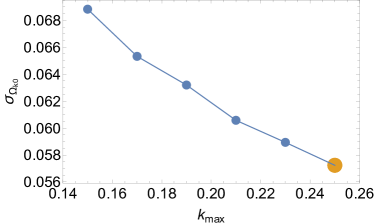
Figure 2: Scaling of $\sigma_{\Omega_{k0}}$ versus $k_{\rm max}$ for the spectrum (keeping fixed to $k_{\rm max}=0.10h/$Mpc the bispectrum value). The bigger yellow dot represents our reference value. The method has only a weak sensitivity to $k_{\rm max}$ values.

One can further improve these constraints in a number of ways, e.g. by adding other redshift bins or larger sky areas, or combining different tracers of structure.

One can also consider external constraints on $H,D$ from standard candles or cosmic chronometers. We tested adding strong external priors for either distance or expansion constraints. We find that FreePower benefits the most from the former: external distance data could improve precision by a factor of almost three. However this comes at the cost of assuming these independently measured distances are free of biases and systematic effects in general.

Appendix A Constraints on $\Omega_{k0}$ assuming $\Lambda$CDM

The results shown in this letter are obtained using the FreePower method where the linear power spectrum is not fixed by cosmology, while standard LSS analyses usually assume a specific model, $\Lambda$CDM, [35, 46, 47, 48, 49, 50, 51], or its generalizations, e.g. see [52, 53, 54]. We perform a Fisher analysis using the same specifications and fiducial values listed in Table 1 adopting $\Lambda$CDM plus a non-zero $\Omega_{k0}$. We use the code PyBird [55] (https://github.com/pierrexyz/pybird), re-adapted to match the biasing scheme of FreePower. We vary simultaneously the cosmology, the bias and the small scales parameters.

It has been observed that, at the scales considered, the one-loop power spectrum and the tree-level bispectrum are not very sensitive to some of the EFT parameters, such as the non-linear bias(es), the counterterms and the shot noise, that are usually fixed or marginalized, see [35, 50]. For this reason we fix the third order bias, the next-to-next-to-leading order counterterm and the scale dependent shot noise [55], while we leave free to vary all the other bias parameters (a total of seven) in each redshift bin. We consider the monopole and quadrupole of the two statistics, neglecting the correlation among different redshift bins as this effect has been shown to be negligible [56].

The results of this $\Lambda$CDM forecast are reported in Tables 3–4. Adding the bispectrum does not significantly improve the constraints on the curvature parameter: with $P$ alone we obtain $\sigma_{\Omega_{k0}}=0.037\;(0.073)$ at 68$\%$ (95$\%$) CL while with $P+B$ we have $\sigma_{\Omega_{k0}}=0.033\;(0.065)$ at 68$\%$ (95$\%$) CL. These results are in line with the analysis performed in [57], and analogous analyses have shown that the bispectrum is essential to constrain the non-linear biases but adds little information about cosmology compared to the $P$ only case [48]. Furthermore, if we include Planck CMB data [2] we obtain $\sigma_{\Omega_{k0}}=0.0021$, ten times better than LSS alone. This results illustrate how, assuming a particular model, the combination of LSS and CMB data is capable of breaking important degeneracies among the cosmological parameters.

References

- [1] Boomerang Collaboration, P. de Bernardis et al., A Flat universe from high resolution maps of the cosmic microwave background radiation, Nature 404 (2000) 955–959, [astro-ph/0004404].
- [2] Planck Collaboration, Planck Collaboration VI, Planck 2018 results. VI. Cosmological parameters, Astron. Astrophys. 641 (2020) A6, [arXiv:1807.06209]. [Erratum: Astron.Astrophys. 652, C4 (2021)].
- [3] E. Calabrese, A. Slosar, A. Melchiorri, G. F. Smoot, and O. Zahn, Cosmic Microwave Weak lensing data as a test for the dark universe, Phys. Rev. D 77 (2008) 123531, [arXiv:0803.2309].
- [4] Planck Collaboration, N. Aghanim et al., Planck 2018 results. VI. Cosmological parameters, arXiv:1807.06209.
- [5] E. Di Valentino, A. Melchiorri, and J. Silk, Planck evidence for a closed Universe and a possible crisis for cosmology, Nat. Astron. (2019) [arXiv:1911.02087].
- [6] D. Sapone, E. Majerotto, and S. Nesseris, Curvature versus distances: Testing the FLRW cosmology, Phys. Rev. D 90 (2014), no. 2 023012, [arXiv:1402.2236].
- [7] R.-G. Cai, Z.-K. Guo, and T. Yang, Null test of the cosmic curvature using and supernovae data, Phys. Rev. D 93 (2016), no. 4 043517, [arXiv:1509.06283].
- [8] Z. Li, G.-J. Wang, K. Liao, and Z.-H. Zhu, Model-independent estimations for the curvature from standard candles and clocks, Astrophys. J. 833 (2016), no. 2 240, [arXiv:1611.00359].
- [9] J. F. Jesus, R. Valentim, P. H. R. S. Moraes, and M. Malheiro, Kinematic Constraints on Spatial Curvature from Supernovae Ia and Cosmic Chronometers, Mon. Not. Roy. Astron. Soc. 500 (2020), no. 2 2227–2235, [arXiv:1907.01033].
- [10] S. Cao, J. Ryan, and B. Ratra, Using Pantheon and DES supernova, baryon acoustic oscillation, and Hubble parameter data to constrain the Hubble constant, dark energy dynamics, and spatial curvature, Mon. Not. Roy. Astron. Soc. 504 (2021), no. 1 300–310, [arXiv:2101.08817].
- [11] S. Dhawan, J. Alsing, and S. Vagnozzi, Non-parametric spatial curvature inference using late-Universe cosmological probes, Mon. Not. Roy. Astron. Soc. 506 (2021), no. 1 L1–L5, [arXiv:2104.02485].
- [12] A. Favale, A. Gómez-Valent, and M. Migliaccio, Cosmic chronometers to calibrate the ladders and measure the curvature of the Universe. A model-independent study, arXiv:2301.09591.
- [13] H. Yu, B. Ratra, and F.-Y. Wang, Hubble Parameter and Baryon Acoustic Oscillation Measurement Constraints on the Hubble Constant, the Deviation from the Spatially Flat CDM Model, the Deceleration–Acceleration Transition Redshift, and Spatial Curvature, Astrophys. J. 856 (2018), no. 1 3, [arXiv:1711.03437].
- [14] J. Ryan, S. Doshi, and B. Ratra, Constraints on dark energy dynamics and spatial curvature from Hubble parameter and baryon acoustic oscillation data, Mon. Not. Roy. Astron. Soc. 480 (2018), no. 1 759–767, [arXiv:1805.06408].
- [15] A. Rana, D. Jain, S. Mahajan, and A. Mukherjee, Constraining cosmic curvature by using age of galaxies and gravitational lenses, JCAP 03 (2017) 028, [arXiv:1611.07196].
- [16] M. Moresco et al., Unveiling the Universe with emerging cosmological probes, Living Rev. Rel. 25 (2022), no. 1 6, [arXiv:2201.07241].
- [17] S. Räsänen, K. Bolejko, and A. Finoguenov, New Test of the Friedmann-Lemaître-Robertson-Walker Metric Using the Distance Sum Rule, Phys. Rev. Lett. 115 (2015), no. 10 101301, [arXiv:1412.4976].
- [18] DESI Collaboration, A. G. Adame et al., DESI 2024 VI: Cosmological Constraints from the Measurements of Baryon Acoustic Oscillations, arXiv:2404.03002.
- [19] C. D. Leonard, P. Bull, and R. Allison, Spatial curvature endgame: Reaching the limit of curvature determination, Phys. Rev. D 94 (2016), no. 2 023502, [arXiv:1604.01410].
- [20] A. Witzemann, P. Bull, C. Clarkson, M. G. Santos, M. Spinelli, and A. Weltman, Model-independent curvature determination with 21 cm intensity mapping experiments, Mon. Not. Roy. Astron. Soc. 477 (2018), no. 1 L122–L127, [arXiv:1711.02179].
- [21] J.-J. Wei, Model-independent Curvature Determination from Gravitational-Wave Standard Sirens and Cosmic Chronometers, Astrophys. J. 868 (2018), no. 1 29, [arXiv:1806.09781].
- [22] V. Alfradique, M. Quartin, L. Amendola, T. Castro, and A. Toubiana, The lure of sirens: joint distance and velocity measurements with third generation detectors, Mon. Not. Roy. Astron. Soc. 517 (2022) [arXiv:2205.14034].
- [23] M. Quartin, L. Amendola, and B. Moraes, The 6x2pt method: supernova velocities meet multiple tracers, Mon. Not. Roy. Astron. Soc. 512 (2022) 2841–2853, [arXiv:2111.05185].
- [24] Y. Yang and Y. Gong, Measurement on the cosmic curvature using the Gaussian process method, Mon. Not. Roy. Astron. Soc. 504 (2021), no. 2 3092–3097, [arXiv:2007.05714].
- [25] B. L’Huillier and A. Shafieloo, Model-independent test of the FLRW metric, the flatness of the Universe, and non-local measurement of , JCAP 01 (2017) 015, [arXiv:1606.06832].
- [26] M. Takada and O. Dore, Geometrical Constraint on Curvature with BAO experiments, Phys. Rev. D 92 (2015), no. 12 123518, [arXiv:1508.02469].
- [27] S. Vagnozzi, E. Di Valentino, S. Gariazzo, A. Melchiorri, O. Mena, and J. Silk, The galaxy power spectrum take on spatial curvature and cosmic concordance, Phys. Dark Univ. 33 (2021) 100851, [arXiv:2010.02230].
- [28] M. Kamionkowski and A. G. Riess, The Hubble Tension and Early Dark Energy, Ann. Rev. Nucl. Part. Sci. 73 (2023) 153–180, [arXiv:2211.04492].
- [29] H. Gil-Marín, W. J. Percival, L. Verde, J. R. Brownstein, C.-H. Chuang, F.-S. Kitaura, S. A. Rodríguez-Torres, and M. D. Olmstead, The clustering of galaxies in the SDSS-III Baryon Oscillation Spectroscopic Survey: RSD measurement from the power spectrum and bispectrum of the DR12 BOSS galaxies, Mon. Not. Roy. Astron. Soc. 465 (2017), no. 2 1757–1788, [arXiv:1606.00439].
- [30] L. Amendola and M. Quartin, Measuring the Hubble function with standard candle clustering, Mon. Not. Roy. Astron. Soc. 504 (2021), no. 3 3884–3889, [arXiv:1912.10255].
- [31] L. Amendola, M. Pietroni, and M. Quartin, Fisher matrix for the one-loop galaxy power spectrum: measuring expansion and growth rates without assuming a cosmological model, JCAP 11 (2022) 023, [arXiv:2205.00569].
- [32] L. Amendola, M. Marinucci, M. Pietroni, and M. Quartin, Improving precision and accuracy in cosmology with model-independent spectrum and bispectrum, JCAP 01 (2024) 001, [arXiv:2307.02117].
- [33] G. D’Amico, M. Marinucci, M. Pietroni, and F. Vernizzi, The large scale structure bootstrap: perturbation theory and bias expansion from symmetries, Journal of Cosmology and Astroparticle Physics 2021 (oct, 2021) 069.
- [34] A. Kiakotou, Ø. Elgarøy, and O. Lahav, Neutrino Mass, Dark Energy, and the Linear Growth Factor, Phys. Rev. D 77 (2008) 063005, [arXiv:0709.0253].
- [35] M. M. Ivanov, M. Simonović, and M. Zaldarriaga, Cosmological Parameters from the BOSS Galaxy Power Spectrum, JCAP 05 (2020) 042, [arXiv:1909.05277].
- [36] A. Chudaykin and M. M. Ivanov, Measuring neutrino masses with large-scale structure: Euclid forecast with controlled theoretical error, JCAP 11 (2019) 034, [arXiv:1907.06666].
- [37] DESI Collaboration, A. Aghamousa et al., The DESI Experiment Part I: Science,Targeting, and Survey Design, arXiv:1611.00036.
- [38] DESI Collaboration, M. Vargas-Magaña, D. D. Brooks, M. M. Levi, and G. G. Tarle, Unraveling the Universe with DESI, in 53rd Rencontres de Moriond on Cosmology, pp. 11–18, 2018. arXiv:1901.01581.
- [39] DESI Collaboration, A. G. Adame et al., DESI 2024 III: Baryon Acoustic Oscillations from Galaxies and Quasars, arXiv:2404.03000.
- [40] EUCLID Collaboration, R. Laureijs, J. Amiaux, S. Arduini, J. L. Auguères, J. Brinchmann, R. Cole, M. Cropper, C. Dabin, et al., Euclid definition study report, arXiv:1110.3193.
- [41] I. S. Matos, M. Quartin, L. Amendola, M. Kunz, and R. Sturani, A model-independent tripartite test of cosmic distance relations, arXiv:2311.17176.
- [42] H. Magira, Y. P. Jing, and Y. Suto, Cosmological redshift-space distortion on clustering of high-redshift objects: correction for nonlinear effects in power spectrum and tests with n-body simulations, Astrophys. J. 528 (2000) 30, [astro-ph/9907438].
- [43] L. Amendola, C. Quercellini, and E. Giallongo, Constraints on perfect fluid and scalar field dark energy models from future redshift surveys, Mon. Not. Roy. Astron. Soc. 357 (2005) 429–439, [astro-ph/0404599].
- [44] L. Samushia et al., Effects of cosmological model assumptions on galaxy redshift survey measurements, Mon. Not. Roy. Astron. Soc. 410 (2011) 1993–2002, [arXiv:1006.0609].
- [45] T. Hahn, Cuba—a library for multidimensional numerical integration, Computer Physics Communications 168 (Jun, 2005) 78–95.
- [46] O. H. E. Philcox, M. M. Ivanov, M. Simonović, and M. Zaldarriaga, Combining Full-Shape and BAO Analyses of Galaxy Power Spectra: A 1.6\% CMB-independent constraint on H0, JCAP 05 (2020) 032, [arXiv:2002.04035].
- [47] M. M. Ivanov, O. H. E. Philcox, T. Nishimichi, M. Simonović, M. Takada, and M. Zaldarriaga, Precision analysis of the redshift-space galaxy bispectrum, Phys. Rev. D 105 (2022), no. 6 063512, [arXiv:2110.10161].
- [48] O. H. E. Philcox, M. M. Ivanov, G. Cabass, M. Simonović, M. Zaldarriaga, and T. Nishimichi, Cosmology with the redshift-space galaxy bispectrum monopole at one-loop order, Phys. Rev. D 106 (2022), no. 4 043530, [arXiv:2206.02800].
- [49] M. M. Ivanov, O. H. E. Philcox, G. Cabass, T. Nishimichi, M. Simonović, and M. Zaldarriaga, Cosmology with the galaxy bispectrum multipoles: Optimal estimation and application to BOSS data, Phys. Rev. D 107 (2023), no. 8 083515, [arXiv:2302.04414].
- [50] G. D’Amico, J. Gleyzes, N. Kokron, K. Markovic, L. Senatore, P. Zhang, F. Beutler, and H. Gil-Marín, The Cosmological Analysis of the SDSS/BOSS data from the Effective Field Theory of Large-Scale Structure, JCAP 05 (2020) 005, [arXiv:1909.05271].
- [51] G. D’Amico, Y. Donath, M. Lewandowski, L. Senatore, and P. Zhang, The BOSS bispectrum analysis at one loop from the Effective Field Theory of Large-Scale Structure, arXiv:2206.08327.
- [52] G. D’Amico, Y. Donath, L. Senatore, and P. Zhang, Limits on clustering and smooth quintessence from the EFTofLSS, JCAP 03 (2024) 032, [arXiv:2012.07554].
- [53] M. M. Ivanov, E. McDonough, J. C. Hill, M. Simonović, M. W. Toomey, S. Alexander, and M. Zaldarriaga, Constraining Early Dark Energy with Large-Scale Structure, Phys. Rev. D 102 (2020), no. 10 103502, [arXiv:2006.11235].
- [54] L. Piga, M. Marinucci, G. D’Amico, M. Pietroni, F. Vernizzi, and B. S. Wright, Constraints on modified gravity from the BOSS galaxy survey, JCAP 04 (2023) 038, [arXiv:2211.12523].
- [55] G. D’Amico, L. Senatore, and P. Zhang, Limits on CDM from the EFTofLSS with the PyBird code, JCAP 01 (2021) 006, [arXiv:2003.07956].
- [56] A. Bailoni, A. Spurio Mancini, and L. Amendola, Improving Fisher matrix forecasts for galaxy surveys: window function, bin cross-correlation, and bin redshift uncertainty, Mon. Not. Roy. Astron. Soc. 470 (2017), no. 1 688–705, [arXiv:1608.00458].
- [57] A. Chudaykin, K. Dolgikh, and M. M. Ivanov, Constraints on the curvature of the Universe and dynamical dark energy from the Full-shape and BAO data, Phys. Rev. D 103 (2021), no. 2 023507, [arXiv:2009.10106].