Gaussian Process Approach for Model-Independent Reconstruction of Gravity with Direct Hubble Measurements
Abstract
Abstract :-
The increase of discrepancy in the standard procedure to choose the arbitrary functional form of the Lagrangian motivates us to solve this issue in modified theories of gravity. In this regard, we investigate the Gaussian process (GP), which allows us to eliminate this issue in a model-independent way. In particular, we use the 57 Hubble measurements coming from cosmic chronometers and the radial Baryon acoustic oscillations (BAO) to reconstruct and its derivatives , , which resulting lead us to reconstruct region of , without any assumptions. The obtained mean curve along CDM constant in the reconstructed region follows a quadratic behavior. This motivates us to propose a new parametrization, i.e., , with the single parameter , which signifies the deviations from CDM cosmology. Further, we probe the widely studied power-law and exponential models against the reconstructed region and can improve the parameter spaces significantly compared with observational analysis. In addition, the direct Hubble measurements, along with the reconstructed function, allow the tension to be alleviated.
Keywords: Gravity — Gaussian Processes Regression — Observational Hubble Data — Cosmology
I Introduction
In contemporary cosmology, the adoption of modified gravity theories has proven highly efficacious in explaining the late-time and near-time acceleration of the Universe [1, 2], circumventing the need for postulating dark energy or inflationary components [3, 4, 5, 6, 7]. Recently, with the mounting discrepancy in the Hubble constant (), researchers have become increasingly inclined to investigate modified gravity as a means to resolve cosmological tension [8, 9, 10]. This motivation arises from the inadequacy of the CDM (Lambda Cold Dark Matter) model in addressing these tensions [11]. Numerous modified gravity theories have been proposed in the literature, with a recent emphasis on a theory rooted in non-metric scalar , which is solely geometric in nature [12]. This modified gravity theory is developed under the assumptions of torsionlessness and a vanishing Ricci scalar.
In contemporary discourse, this modified theory of gravity is in high demand due to its successful portrayal of various cosmological scenarios. Extensive research has been conducted within this framework to address current cosmological issues [13, 14, 15, 16, 17, 18, 19, 20, 21]. Additionally, several modifications or extensions of this theory, such as gravity [22] and gravity [23, 24], have been proposed. However, a fundamental challenge associated with modified gravity theories lies in the arbitrary selection of a function governing the nonmetricity scalar . This approach often necessitates making numerous assumptions and lacks inherent symmetry.
Furthermore, observational data are employed to constrain the cosmological models involving and to estimate the requisite parameters for desired outcomes [13, 14, 25]. Various methodologies exist for discussing the cosmophysical properties, including assuming specific forms of , studying the dynamical behavior of backgrounds and perturbations, and validating outcomes through observational testing, including comparisons with the solar system [19, 26, 27].
While these methodologies provide valuable insights, advancements in learning have facilitated a process whereby the function can be constructed using observational measurements without presupposing a particular form. This reconstruction process, known as the Gaussian Process (GP) method, has been successfully developed and utilized across various studies [28, 29, 30]. This method has been studied and explored in various dark energy scenarios such as (see the references herein [31, 32, 33, 34, 35, 36, 37]) and the expansion history of the universe [38, 39, 40, 41, 42]. This procedure allows for the reconstruction of in a model-independent manner, thereby enhancing the robustness of cosmological analyses. Consequently, the GP process is poised to play a pivotal role in modern cosmological inquiries, enabling the representation of reconstructions in terms of uncertainty and offering a means to reconstruct without assuming specific conditions.
The investigation in this study unfolds across several sequential stages. Initially, we provide a succinct overview of the symmetric teleparallel gravity framework for the FLRW spacetime metric in Section II, succeeded by an exploration of Gaussian processes with a focus on reconstructing the Hubble parameter and its derivative in Section III. Moving to Section IV, we meticulously outline the step-by-step procedures employed in the reconstruction process of , also confronted particular selections for against it. Additionally, we delve into cosmological applications to corroborate the prevailing state of the universe. Finally, in Section V, we encapsulate our findings and contemplate future perspectives.
II Gravity Theory
We begin this section by discussing the metric affine connection - a fundamental mathematical tool in differential geometry and general relativity, providing a framework for understanding the geometry of curved manifolds equipped with both metric and affine structures. To investigate the cosmological aspects of non-metric gravity, let us examine the most general form of the affine connections
| (1) |
where the Levi-Civita connection is defined as
| (2) |
which can be uniquely determined by the first-order derivatives of the metric tensor . The contortion and deformation tensor are defined as
respectively, which describes non-Riemannian properties in the manifold. The contortion tensor disappears in the symmetric teleparallel theory because it follows an anti-symmetric property. The interplay between nonmetricity and the absence of torsion would influence cosmological models and the evolution of the universe. These effects could manifest in scenarios such as the dynamics of inflation, the behavior of dark energy, and the formation of large-scale structures.
The non-metricity tensor is defined as
| (3) |
and the corresponding traces are , . Aside from that, the superpotential tensor can be written as
| (4) |
obtaining a trace of nonmetricity tensor or nonmetricity scalar as
| (5) |
In this work, we study the extension of symmetric teleparallel theory called gravity theory, and its considered action is given as [12]
| (6) |
where represents any function of the scalar , denotes the determinant of , and stands for the matter Lagrangian density.
As action (6) varies with respect to the metric, the gravitational field equation for is obtained, and it is written as
| (7) |
where . The energy-momentum tensor for matter is now defined as
.
To utilize gravity in a cosmological context, we adopt the spatially flat Friedmann-Lemaitre-Robertson-Walker (FLRW) spacetime, characterized by a specific metric
| (8) |
corresponding nonmetricity scalar is obtained as , where is the Hubble parameter with denoting cosmological scale factor and the upper dot denotes derivative with respect to the coordinate time . Applying the FLRW metric into the general field equation (7), the relevant Friedman equations of cosmology, namely
| (9) |
| (10) |
where , and . Furthermore, in the equations provided, represents the energy density, and denotes the pressure of the matter fluid. It can be easily derived that they accomplish the conservation equation .
We can rewrite Eqs. (9) and (10) as the standard form
| (11) |
| (12) |
where
| (13) |
| (14) |
are the dark energy density and pressure contributed by the modified part of geometry. Then, by using Eqs. (13) and (14), we can define the effective dark energy equation of state as
| (15) |
Additionally, the conservation equation of the effective dark energy,
| (16) |
In our analysis, we focus on the late-time evolution of the cosmic fluid, so that we can neglect radiation and consider the entire contribution due to pressureless matter. This implies and , where the subscript zero refers to quantities evaluated at the present time, and is the redshift defined as .
III Gaussian Processes Using Observational Hubble Data
III.1 Gaussian Process
A Gaussian process is a type of statistical model that extends a Gaussian distribution. Gaussian process regression is a technique that is commonly used to reconstruct functions and their derivatives directly from observed data without making any assumptions. This process involves gathering a set of random variables that all follow a Gaussian distribution [43]. The relationship between these variables is determined by a covariance matrix function, which is uniquely determined by the data points. As a result, Gaussian processes provide a way to reconstruct functions without relying on any specific physical assumptions or parameterizations.
The Gaussian process is written as [43, 29, 44]
| (17) |
where is the kernel function and are the observational points. The provides the mean of the random variable at each . In this work, we employ the squared exponential function as our kernel function to reconstruct functions and their derivatives [29, 44, 30]. This kernel function represents the most versatile form of covariance function, and it is given by
| (18) |
This kernel function depends on the two hyperparameters and . Specifically, determines the correlation length between consecutive values of , while regulates the variation of in relation to the process mean.
In this study, we utilize the Gaussian Processes in Python (GAPP) developed by Seikel et al. [43], to reconstruct the evolution of the Hubble function and its derivatives from observational Hubble data.
III.2 Observational Hubble Data (OHD)
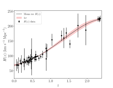
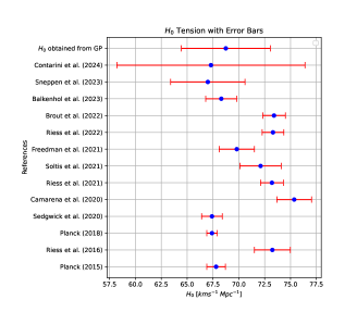
We used the latest 57 points of Hubble data along with their error bars for the Gaussian reconstruction process. Out of these 57 points, 31 were obtained from cosmic chronometer (CC) observations, which provide information on from the age evolution of passively evolving galaxies in a model-independent way. The remaining 26 points were obtained from radial baryon acoustic oscillation (BAO) observations which measure the clustering of galaxies with the BAO peak position as a standard ruler. The BAO peak position depends on the sound horizon. The OHD comprises 57 data points within the redshift range of . The combination of two Hubble samples increases the statistics and helps us to find better results from the GP. From this scrutiny, we determined the value as . We have presented a figure comparing with the recent measurements on in Figure 2. In Table 2 we present the above points along with references. As we are considering the direct and local measurements of the Hubble values; the tension will be alleviated by the modified gravity reconstruction.
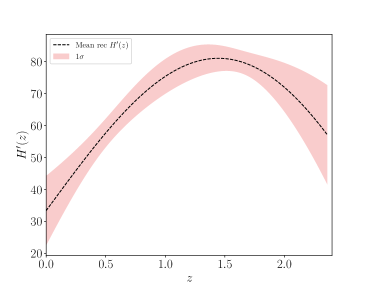
The Hubble parameter and its derivative (prime denote the derivative with respect to ), successfully reconstructed in a model-independent manner, are depicted in Figure 1.
IV Reconstructing the Function from Gaussian Processes Utilizing OHD Data
In this section, we will attempt to derive the functional form of by using the reconstructed Hubble function and its derivative, which we obtained in the previous section by applying the Gaussian process to OHD data. The process of reconstruction is simpler in FLRW cosmology in gravity, as it only depends on the Hubble function and its first-order derivative. Our goal is to establish the relationship between the redshift and , or in other words, to find .
To use the model-independent reconstruction approach, we need first to extract the expressions for the involved derivatives as
| (19) |
where primes represent the derivative with respect to redshift . The following step in the application of the GP is to take the approximation of as
| (20) |
for small . Using the modified Friedmann equation (9) and the approximation above for , we can extract a recursive relation between consecutive redshifts ( and ). This involves writing as a function of , and and as
| (21) |
Ultimately, we arrived at the final phrase as follows by using the EoS parameter for the matter sector:
| (22) |
Utilizing the provided expression, we can compute the value of at the redshift , given that we possess information about the parameters at redshift . Furthermore, through an analysis of the connection between and , and by observing the evolution of , we can derive the expression of in relation to redshift .
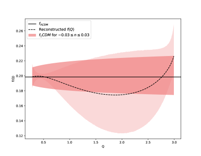
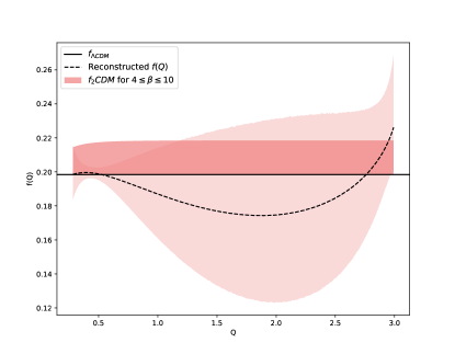
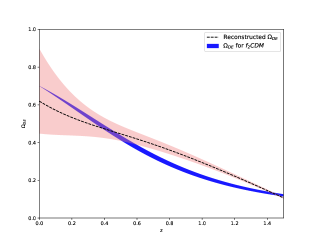
In Figure 3, we present the reconstructed function using the GP against . Now, our aim find the appropriate functional form of from our results, which will able to mimic the reconstructed .
In the reconstruction profile, we presented the mean reconstruction curve alongside the CDM model depicted by the straight line. This line maintains a constant value of , derived from the analysis. Observably, the reconstructed mean curve does not hold a constant value like , but rather embodies the best-fit curve from the Gaussian analysis. It adopts a second-order polynomial form as , with the parameter values and , constrained by the reconstructed data. Notably, the functional form of simplifies to , Consequently, the reconstructed functional form now relies solely on one parameter, , as the linear term merges with the standard linear form in the action. Although one could introduce additional parameters into the reconstructed function, but a model with fewer parameters typically represents a better model than one with more. Therefore, we adhere to the one free parameter form of denoted as
| (23) |
Subsequently, the reconstructed curve , along with its shaded error regions, aids in discerning the true form of some widely studied functions of . To this end, we compare two models: a power law-type and an exponential type, in search of suitable functions.
IV.1 CDM :-
First, we consider the power-law model (CDM) [13, 19, 27], which is of the form , with .
When , the model reduces to , which recover the CDM expansion history of the universe.
It’s worth noting that any curve falling within the shaded area in Figure 3 can be considered the true form of , besides the mean reconstruction curve. Hence, we constrain the free parameter to determine which values of allow the CDM model to fit within the reconstructed area. As shown in Figure 3a, the constraint value indicates that might fall between the range of .
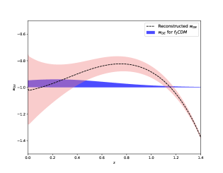
The DE equation of state parameter corresponding to CDM is
| (24) |
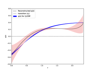
and the deceleration parameter is
| (25) |
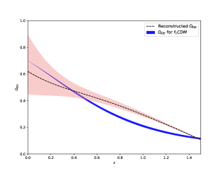
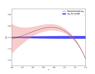
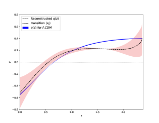
IV.2 CDM :-
Next, we consider the exponential model (CDM) [47, 46, 27], which is of the form , with . For the model reduces to the symmetric teleparallel theory equivalent to GR without a cosmological constant. When , the model reduces to , which recover the CDM expansion history of the universe.
Here also, we constrain the free parameter to determine which values of allow the CDM model to fit within the reconstructed area. As shown in Figure 3b, the constraint value indicates that might fall between the range of .
The DE equation of state parameter corresponding to CDM is
| (26) |
and the deceleration parameter is
| (27) |
| Model | |||
|---|---|---|---|
| Reconstructed | |||
| CDM | |||
| CDM |
V Conclusion
In this manuscript, we have independently reconstructed the function using observational measurements. To achieve this objective, we have incorporated local Hubble measurements, including Cosmic Chronometers and Baryon Acoustic Oscillations (BAO), and employed Gaussian Processes (GP) for statistical analysis. Recent inquiries into modified gravities have spurred the search for a function derivable from observational data. Typically, researchers assume specific functional forms for and then constrain the free parameters using observational measurements, often arbitrary assumptions. However, the GP methodology allows us to discern the functional form of independently, without imposing specific conditions based on observational measurements.
Our analysis encompasses Hubble measurements, encompassing Cosmic Chronometers and BAO measurements, for GP analysis. From this scrutiny, we determined the value of , which not only resolves the tension issue in a model-independent manner but also aligns closely with recent precise studies on the subject. To advance our investigation, we first reconstructed and its first derivative from observational samples. Given that the non-metric scalar is a function of , all Friedmann equations can be expressed in terms of and its first derivative . Leveraging the reconstructed functions of and its derivative , we reconstructed without resorting to any assumptions. This reconstructed addresses the issue by employing local Hubble measurements.
Figure 3 displays the profile of the reconstructed function concerning the non-metricity scalar , where the dark dotted line represents the mean reconstructed function, the shaded region denotes the error, and the black line indicates the CDM model. The deviation of the reconstructed function from CDM suggests a quadratic behavior, leading us to propose a quadratic functional form of with a single free parameter, quantifying the deviation from CDM as . Furthermore, we constrain the range of this free parameter within which the one-parameter function lies in the reconstructed region given by .
Additionally, we scrutinized two widely studied forms of against the reconstructed function, enhancing the constraint on the free parameters compared to traditional observational constraints, and presented the improved parameter range. Moreover, we explore cosmological implications, investigating deceleration parameters, dimensionless dark energy, and the dark energy equation of state parameters for specific models. As anticipated, our findings corroborate the current accelerated expansion of the universe, consistent with recent studies.
In conclusion, our study presents a model-independent reconstruction and proposition of the functional form, solely relying on observational measurements through GP analysis. This approach not only enhances constraints on the free parameters of specific models but also circumvents arbitrary choices for gravitational Lagrangian functions. While our study focuses on Hubble measurements, future endeavors could extend this analysis to other observational measurements, such as supernovae, which we aspire to explore in forthcoming research.
Data Availability Statement
There are no new data associated with this article.
Acknowledgments
GNG acknowledges University Grants Commission (UGC), New Delhi, India for awarding Junior Research Fellowship (UGC-Ref. No.: 201610122060). SM acknowledges the Japan Society for the Promotion of Science (JSPS) for providing postdoctoral felowship. PKS acknowledges Science and Engineering Research Board, Department of Science and Technology, Government of India for financial support to carry out Research project No.: CRG/2022/001847 and IUCAA, Pune, India for providing support through the visiting Associateship program.
References
- [1] S. Capozziello, and M. De Laurentis, Phys. Rept. 509, 167 (2011).
- [2] S. Nojiri, and S. D. Odintsov, Phys. Rept. 505, 59 (2011).
- [3] P. J. E. Peebles, and B. Ratra, Rev. Mod. Phys. 75, 559 (2003).
- [4] Y. F. Cai, E. N. Saridakis, M. R. Setare and J. Q. Xia, Phys. Rept. 493, 1 (2010).
- [5] X. Li, A. Shafieloo, Astrophys. J. Lett. 883(1), L3 (2019).
- [6] X. L. Li, A. Shafieloo, V. Sahni, and A. A. Starobinsky, Astrophys. J., 887:153 (11pp) (2019).
- [7] E. Elizalde, M. Khurshudyan, and S. Nojiri, Int. J. Mod. Phys. D 28, no.01, 1950019 (2018).
- [8] K. C. Wong et al., Mon. Not. Roy. Astro. Soc. 498, 1 (2020).
- [9] W. L. Freedman et al., Astrophys. J. 882, 1 (2019).
- [10] S. Vagnozzi, Phys. Rev. D 102, 023518 (2020).
- [11] Y. F. Cai, S. Capozziello, M. De Laurentis and E. N. Saridakis, Rept. Prog. Phys. 79, no. 10, 106901 (2016).
- [12] J. B. Jimenez et al., Phys. Rev. D 98, 044048 (2018).
- [13] R. Lazkoz et al. Phys. Rev. D 100, 104027, (2019).
- [14] Fotios K. Anagnostopoulos et al., Phys. Lett. B. 822, 136634, (2021).
- [15] N. Frusciante, Phys. Rev. D 103, 044021, (2021).
- [16] R. H. Lin, and X. H. Zhai, Phys. Rev. D 103, 124001, (2021).
- [17] S. Mandal et al., Phys. Rev. D 102, 024057 (2020).
- [18] S. Mandal et al., Phys. Rev. D 102, 124029 (2020).
- [19] J. B. Jimenez et al., Phys. Rev. D 101, 103507, (2020).
- [20] T. Harko et al., Phys. Rev. D 98, 084043, (2018).
- [21] L. Heisenberg, arXiv: 2309.15958.
- [22] Y. Xu et al., Eur. Phys. J. C 79, 708 (2019).
- [23] S. Capozziello, V. De Falco, and C. Ferrara, Eur. Phys. J. C 83, 915 (2023).
- [24] Avik De et al., JCAP 03, 050 (2024).
- [25] I. Ayuso, R. Lazkoz, and V. Salzano, Phys. Rev. D 103, 063505 (2021).
- [26] W. Khyllep, A. Paliathanasis, and J. Dutta, Phys. Rev. D 103, 103521 (2021).
- [27] W. Khyllep et al., Phys. Rev. D 107, 044022 (2023).
- [28] T. Holsclaw, et al., Phys. Rev. Lett. 105, 241302 (2010).
- [29] C.E. Rasmussen, and C.K. Williams, 2005, Gaussian Processes for Machine Learning (Cambridge, MA: MIT Press)
- [30] M. Seikel, and C. Clarkson, 2013, arXiv:1311.6678
- [31] F. Melia, and M. K. Yennapureddy, JCAP 02, no. 02, 034 (2018).
- [32] A. M. Pinho, S. Casas, and L. Amendola, JCAP 11, no. 11, 027 (2018).
- [33] M. J. Zhang, and H. Li, Eur. Phys. J. C 78, no. 6, 460 (2018).
- [34] Z. Y. Yin, and H. Wei, Sci. China Phys. Mech. Astron. 62, no. 9, 999811 (2019).
- [35] E. Elizalde, and M. Khurshudyan, Phys. Rev. D 99, no. 10, 103533 (2019).
- [36] M. M. Rau, S. Wilson, and R. Mandelbaum, Mon. Not. Roy. Astron. Soc., 491, 4 (2020).
- [37] A. Gomez-Valent, and L. Amendola, JCAP, 1804, 051 (2018).
- [38] V.C. Busti, C. Clarkson, and M. Seikel, Mont. Not. Roy. Astron. Soc. 441, 11 (2014).
- [39] L. Verde, P. Protopapas, and R. Jimenez, Phys. Dark Univ. 5, 307 (2014).
- [40] Z. Li et al., Phys. Rev. D 93, 043014 (2016).
- [41] D. Wang, and X.H. Meng, Sci. China Phys. Mech. Astron. 60, 110411 (2017).
- [42] F. Melia, and M.K. Yennapureddy, J. Cosmol. Astropart. Phys. 02, 034 (2018).
- [43] M. Seikel, C. Clarkson, and M. Smith, J. Cosmol. Astropart. Phys., 06, 036, (2012).
- [44] A. Mehrabi, and M. Rezaei, Astrophys. J. 923, 274 (2021).
- [45] S. Contarini et al., Astron. Astrophys. 682, A20 (2024); A.G. Riess et al., Astrophys. J. L. 908, L6 (2021); J. Soltis, S. Casertano, and A.G. Riess, Astrophys. J. L. 908, L5 (2021); W.L. Freedman, Astrophys. J. 919, 16 (2021); L. Balkenhol et al., Phys. Rev. D 108, 023510 (2023); Dillon Brout et al., Astrophys. J. 938, 110 (2022); Sneppen et al., Astron. Astrophys. 678, A14 (2023); A.G. Riess et al. Astrophys. J. L. 934, L7 (2022).
- [46] F. A. Anagnostopoulos et al., Eur. Phys. J. C 83, 58 (2023).
- [47] O. Sokoliuk et al., Mon. Not. Roy. Astron. Soc. 522, 252–267 (2023).
- [48] Stern D. et al., J. Cosmol. Astropart. Phys. 02, 008, (2010)
- [49] Simon J., Verde L. , Jimenez R. , Phys. Rev. D 71, 123001, (2005)
- [50] Moresco M. et al., J. Cosmol. Astropart. Phys. 08, 006, (2012)
- [51] Zhang C. et al., Research in Astron. and Astrop. 14, 1221, (2014)
- [52] Moresco M. et al., J. Cosmol. Astropart. Phys. 05, 014, (2016)
- [53] Ratsimbazafy A. L. et al., Mon. Not. Roy. Astron. Soc. 467, 3239, (2017)
- [54] Moresco M., Mon. Not. Roy. Astron. Soc. Lett. 450, L16, (2015)
- [55] Gaztaaga E. et al., Mon. Not. Roy. Astron. Soc. 399, 1663, (2009)
- [56] Oka A. et al., Mon. Not. Roy. Astron. Soc. 439, 2515, (2014)
- [57] Wang Y. et al., Mon. Not. Roy. Astron. Soc. 469, 3762, (2017)
- [58] Chuang C. H., Wang Y., Mon. Not. Roy. Astron. Soc. 435, 255, (2013)
- [59] Alam S. et al., Mon. Not. Roy. Astron. Soc. 470, 2617, (2017)
- [60] Blake C. et al., Mon. Not. Roy. Astron. Soc. 425, 405, (2012)
- [61] Chuang C. H. et al., Mon. Not. Roy. Astron. Soc. 433, 3559, (2013)
- [62] Anderson L. et al., Mon. Not. Roy. Astron. Soc. 441, 24, (2014)
- [63] Busca N. G. et al., Astron. Astrophys. 552, A96, (2013)
- [64] Bautista J. E. et al., Astron. Astrophys. 603, A12, (2017)
- [65] Delubac T. et al., Astron. Astrophys. 574, A59, (2015)
- [66] Font-Ribera A. et al., J. Cosmol. Astropart. Phys. 05, 027, (2014)
Appendix
| Table-1: datasets consisting of 57 data points | |||||||
| CC data (31 points) | |||||||
| Ref. | Ref. | ||||||
| [48] | [52] | ||||||
| [49] | [48] | ||||||
| [48] | [50] | ||||||
| [49] | [50] | ||||||
| [50] | [50] | ||||||
| [50] | [50] | ||||||
| [51] | [48] | ||||||
| [49] | [49] | ||||||
| [51] | [50] | ||||||
| [50] | [49] | ||||||
| [52] | [54] | ||||||
| [49] | [49] | ||||||
| [52] | [49] | ||||||
| [52] | [49] | ||||||
| [52] | [54] | ||||||
| [53] | |||||||
| From BAO & other method (26 points) | |||||||
| Ref. | Ref. | ||||||
| [55] | [57] | ||||||
| [56] | [57] | ||||||
| [57] | [61] | ||||||
| [55] | [62] | ||||||
| [58] | [57] | ||||||
| [57] | [60] | ||||||
| [59] | [59] | ||||||
| [57] | [57] | ||||||
| [55] | [60] | ||||||
| [60] | [63] | ||||||
| [57] | [64] | ||||||
| [57] | [65] | ||||||
| [59] | [66] | ||||||