Regularization techniques for estimating the source in a complete parabolic equation in
1 Introduction
Complete parabolic equations are used to model transport phenomena. These are highly studied due to the number of direct applications they are related to in different fields of physics, as they are used to analyze the transfer of mass, energy, and information in different processes [1, 2]. Among the most important applications, we can mention the heat transfer of a body immersed in a moving fluid [3], heat transfer in biological tissue [4], and the concentration of a certain compound in a flow of water [5].
On the other hand, the problem of source determination has been analyzed in recent years in various areas of applied physics and has garnered considerable attention in current research. It finds applications in fields such as heat conduction [6, 7, 8, 9], crack identification [10], electromagnetic theory [11, 12, 13], geophysical prospecting [14], contaminant detection [15], and detection of tumor cells [16], among others.
Several methods are available in the literature for determining a source, and among the most important tools are the potential logarithmic method [17], the projective method [18], Green functions [19], limit element methods of dual reciprocity [20], the method of dual reciprocity [21], and the method of fundamental solution [22].
In the context of various transport processes or complete parabolic differential equations, there is a limited number of articles published for the general case [23, 24, 25], with the majority of available literature focusing on the one-dimensional heat equation. Different methods, techniques, and strategies have been employed to retrieve sources in this equation, as seen in [26, 27, 28]. Many articles analyze specific cases with simplifications or restrictions in mathematical models, source types, boundary conditions, or selected domains, such as [26, 27, 28, 29, 30, 31, 32]. The most commonly used methods in these cases include the limit element method [26, 28], the fundamental solution method [27, 32], the Ritz-Galerkin method [33], the finite difference method [34], the meshless method [35], the conditional stability method [36], and the shooting method [29].
The problem of source determination is considered ill-posed in the sense of Hadamard [37], as the solution does not depend continuously on the data. Regularization methods [38, 39] play a crucial role in estimating unstable solutions. Among the most commonly used are the iterative regularization method [40, 41], the simplified Tikhonov regularization method [42, 43, 44, 45, 46], the modified regularization method [8, 25, 46, 47, 48, 49], Fourier truncation [48], and the mollification method [50].
When it comes to source determination in parabolic equations, [51] focuses on a convection-diffusion equation, while [7, 34, 47, 49, 52, 53, 54, 55, 56] exclusively consider diffusion. More recently, the problem of finding the source term in a complete parabolic equation has been addressed using the quasi-reversibility method, as seen in [57]. Notably, this method extends its applicability to solving the inverse source problem in nonlinear parabolic equations [58].
The issue addressed in this article stems from modeling various transportation problems and involves identifying the source term, which is independent of time, in a complete parabolic evolutionary equation using measurements or noisy data taken at an arbitrary fixed time. This problem is ill-posed, as high-frequency components of arbitrarily small data errors can result in disproportionately large errors in the solution. To tackle this challenge, three uniparametric families of regularization operators are devised to counteract the instability of the inverse operator. These regularization operators create families of well-posed problems that approximate the originally ill-posed problem. Additionally, a guideline is provided for selecting the regularization parameter. The stability and convergence of each method are analyzed, and an optimal H”older bound is derived for the error of each estimate.
The three strategies presented here generalize the ideas used by other authors for the case of the one-dimensional heat equation. Here, they are applied to a complete parabolic equation where temperature measurements can be taken at any instant. On the other hand, the proposal is framed within the theory of operators, giving rise to applications in more general contexts and problems. Any important application is the detection of contaminants in groundwater layers, this is a problem that concerns all urbanized cities. Being able to determine the focus of contamination from measurements in a particular place, minimizes the costs used for the search [15, 59, 60]. Another application is the estimation of the metabolic heat in a biological tissue [24] using the Pennes model [4]. Any existing abnormality within the body can lead to variations in temperature and heat flux at the surface. The presence of a tumor produces local inflammation, increased metabolic activity, among other symptoms. Due to this, the diseased cells act as a source of temperature that produces abnormal thermal profiles in the skin and its measurements can be used to identify, locate and characterize the sick cells. The two problems mentioned above can be addressed with the tools that are explained in this paper. There are many other applications in different disciplines, these two are mentioned as an example to highlight the importance of the problem and the proposed methods.
To illustrate the performance of the proposed regularizations and in order to compare the different regularization operators introduced in this article; numerical examples of different characteristics are included.
2 Source identification
In this section, the inverse problem to be studied is formally presented, an analytical expression is given for the solution of the problem of interest, and it is shown that the problem is ill-posed.
2.1 Presentation of the problem
Given , we seek to determine the source term in the following complete parabolic equation in an unbounded domain
| (1) |
where , denote the Laplacian and Nabla operators, respectively, and represents the usual inner product in . Without loss of generality, the null initial condition is considered, i.e.,
| (2) |
The determination of the source term in Equation (1) with the condition (2), is carried out using experimental or simulated noisy data, at an instant of time .
| (3) |
where represents the noisy data or measurements and is the noise in the data. It is also assumed that said noise is bounded, that is,
| (4) |
where is the maximum noise level tolerated. In practice is obtained from measurement, instrumentation and calibration errors.
2.2 Problem solution
The source estimation problem will be solved using the -dimensional Fourier transform. It is included here for completeness reasons.
Definition 1.
Let , the -dimensional Fourier transform [61] is defined by
Let , the Fourier antitransform is defined by
Proposition 1.
The -dimensional Fourier transform is a linear integral operator that satisfies the following property. Let hence:
From the use of the definition 1 and the proposition it is possible to find the analytical solution of the problem of interest given by the equations (1)-(4). This is given in the following result.
Theorem 1 (Solving the source identification problem).
For and such that , are the functions with satisfying the parabolic problem
| (5) |
Then, the expression for the source is given by
where
with
Proof.
For the proof of theorem 1 it is used the -dimensional Fourier transform given in 1 on the space variables of the system (5). Then the proposition 1 is used to obtain,
| (6) |
where is the -dimensional Fourier variable. Equivalently, the identification problem (5) can be rewritten fron (6) in frequency space as follows
| (7) |
where is given by the expression,
| (8) |
The system (7) is represented by a first order non-homogeneous differential equation with initial condition. The analytical solution to this equation is,
| (9) |
Because , evaluating Equation (9) at produces a linear expression for the source in frequency space,
| (10) |
where
| (11) |
| (12) |
which ends the proof. ∎
2.3 Ill-posed problem
The problem of identifying the source in a complete parabolic equation from noisy measurements turns out to be a ill-posed problem in the sense of Hadamard [37] since the solution does not depend continuously on the data. This fact can be seen in the following result.
Theorem 2 (The problem is ill-posed).
Proof.
We denote . It’s easy to see that
| (14) |
from (14) it is evident that is not bounded, since it tends to infinity as . As can be seen in (13) this fact amplifies the error of the measurements at high frequencies and this can lead to a large estimation error even for very small observation or measurement errors. In other words, the solution to the identification problem (5) does not vary continuously with the data (see [38]).
∎
3 Regularization operators
When an inverse problem is ill-posed, a regularization method is usually applied to stabilize the solution. In this section, three regularization operators are proposed for comparative purposes. The existence of the regularization parameter leading to three convergent methods is proved, and basic theoretical issues related to regularization operators are included. Readers unfamiliar with this topic may find more information at[38, 39].
3.1 Regularization solutions
To stabilize the ill-posed problem, regularization operators will be used.
Definition 2.
Let and be Hilbert spaces and a linear bounded operator. A regularization strategy for is a family of linear bounded operators satisfying
For our particular case, the parametric families of linear operators are defined by with and ; such that
| (15) |
where is defined in (11), with , are regularization strategies for and is the regularization parameter.
Note 1.
Note that the denominators of the expressions (15) that define the linear operators with , were introduced in the solution only for stabilization purposes.
Theorem 3 (Convergent regularization operators).
Consider the source identification problem (5). Let that satisfy the following differential equation with initial condition
| (16) |
and let with be the families of operators defined in (15). Then, for all there exists an a priori parameter choice rule for such that the pairs for are convergent regularization methods for the identification problem (16).
Proof.
The operators with defined in (15) are continuous for all and are bounded, since it is evident that,
Therefore, for each parameter , the operators with are linear, continuous and it has to be
where , then with are regularization strategies for . Therefore, according to [38], there exist a priori parameter choice rules such that with are convergent regularization methods to solve (10). ∎
The regularized solution of the inverse source identification problem, in frequency space, is given by
| (17) |
Therefore, from the equation (17) an approximate expression for the function is obtained, solution of the problem given in (16). This is,
equivalently
| (18) |
Using in the equation (18), the definitions of the regularization operators with given by the equations (15), three analytic expressions for the source estimate are obtained (one for each regularization strategy). These are,
and
3.2 Error Analysis
In this section, a bound will be obtained for the error committed by each estimation.
3.2.1 Auxiliary results
In order to analyze the behavior of the proposed regularizations, some results are first introduced that will be used later to obtain an error bound between the source and its estimates
Note 2.
Some of the auxiliary results may seem trivial to the reader. However, and in order to carry out a complete and self-contained work, a brief demonstration is presented for each one of them.
Lemma 1.
Let with then
Proof.
Euler’s formula is used for complex numbers and it is found that,
therefore,
∎
Lemma 2.
The function defined by satisfies .
Proof.
First, consider at . Differentiating, in this case, we have
the function is increasing in . Then
On the other hand, for , we have
the function is decreasing . Then
So, , ∎
Lemma 3.
Let . If we have
Proof.
Lemma 4.
Let . So .
Proof.
Let be defined by . Differentiating we get,
Then, the function is strictly decreasing and also,
Then ∎
Lemma 5.
Let . So .
Proof.
Let be defined by . Differentiating we get,
Then the function has its only critical point at . Noting that and , it follows that is the absolute maximum of . So,
∎
Lemma 6.
Let . If we have Furthermore, for the following inequality is valid
Proof.
For all holds
In addition, since the first inequality is obtained,
On the other hand, let then and has a single critical point . Three cases are considered:
-
•
: we have , constant .
-
•
: then the function reaches its global maximum value at .
-
•
: is an even and increasing function for 0 with we have .
Therefore,
∎
Lemma 7.
Let . If we have Also, for the following inequality is valid
Proof.
For all the lemma 6 is used and the proof is immediate, since
On the other hand, for the case , we have,
∎
Lemma 8.
Proof.
Since the three regularization operators given in (15) contain the expression defined in (11), we begin by bounding this operator. The lemma 1 applied to the absolute value of (11) is used and we immediately obtain,
| (22) |
If : From the inequality (22), using the triangular inequality, the lemma 2 and the lemma 6, we have,
| (23) |
Similarly, from the inequality (22), using the triangular inequality, the lemma 2 and the lemma 7, we obtain,
| (24) |
Finally, from the inequality (22), using the triangular inequality, the lemmas 2, 3, 4 and 5 hold that,
| (25) |
If : From the inequality (22), using the triangular inequality, the lemma 2 and the lemma 6, we have,
Lemma 9.
Proof.
Let
Three cases are considered for the proof.
Case 1 . So
| (30) |
Case 2 . So
| (31) |
| (32) |
| (33) |
Case 3 . So
| (34) |
| (35) |
| (36) |
If you have
| (37) |
If follow that
| (38) |
Remark 1.
Notice that
3.2.2 Analytical bound of error
Now it is possible to obtain a bound for the error estimate.
Definition 3.
The norm in Sobolev space for is defined as
| (39) |
By means of the definition (39), a parameter choice rule is given for the proposed regularizations and an analytical expression is found for the error bound of each estimation. This can be seen in the following result.
Theorem 4 (Analytical bound for the estimation error).
Consider the inverse problem of determining the source in (5). Let with be the regularization solutions given in (18). It is assumed that there exists bounding the norm of in for some (39). if chosen
| (40) |
then there exist constants independent of such that
Proof.
rearranging
We use the definition of the norm in the Sobolev space given by the expression (39),
| (41) |
By the triangle inequality we have,
| (42) |
Remark 2.
Note that the bound (46) satisfies
which means that the estimate () converges to the source function () when the noise in the data () tends to .
Remark 3.
Note that the case is not included in the hypotheses of the 4 theorem, the reason is that in this case,
Remark 4.
Note that the bound obtained for the regularization error (46) is of Hölder type and only depends on the smoothness of the source and the parameters of the mathematical model.
Note 3.
A case of special interest in the bibliography is for . In this the expression (46) is reduced to:
3.3 Numerical examples
We consider concrete examples of the estimation of the source in for . For each of the examples discussed in this section, different values are chosen for the parameters of the source identification problem , . In addition, to simulate the noise in the data, a set of values of standard deviation . The space is discretized into a uniform -dimensional mesh and a data set is obtained from the evaluation of the solution at a fixed time instant given and adding noise, that is,
where is a uniform discretization on chosen and are realizations of the normally distributed random variable with mean 0 and deviation . By denoting and taking into account the noise level satisfying (4), the error
It is numerically calculated using the Simpson integration method. This calculation allows obtaining an approximate value of the error that directly depends of the noise. It can be seen that the noise level is a function of the standard deviation , that is, .
In practice, the maximum tolerance value for the error in the data given in (4) is obtained from the calibration, instrumentation and measurement errors of the instruments used to perform the measurements. Here, to make sure that the regularization parameter is less than 1, it is chosen as the maximum value of plus one unit. That is to say,
Then is calculated using the FFT transform (Fast Fourier Transform) [62] and get the regularization solutions with given in (18) using the anti-fast Fourier transform [7, 62], where the regularization parameter is chosen according to (40), that is to say,
For each of the examples considered, the results of the estimated sources without regularization and those obtained after using the regularization methods presented in this article are graphed. An error table is also included for each example. These tables consider the relative errors made, in the estimation, by each one of the regularization operators used to address the ill-posed problem. The disturbances used for the construction of the tables are , these were chosen based on the values of the solution.
Note 4.
The reader may notice that in some examples the considered for the recovery does not correspond to the space to which the source belongs, since is not in that Hilbert space. These examples were included to show that recovery is reasonable even in those cases.
3.3.1 Examples 1D
In this subsection, three examples of estimation of one-dimensional sources with different characteristics are discussed.
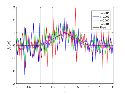
Example 1.
For this example, the following parameters are considered ; ; 1; and . Also, the perturbation values used are 0.05}. Finally, the source to estimate in this case is:
| (47) |
The source (47) retrieved in example 1 is of interest in signal theory. This type of function turns out to be a common example in [48, 50] source retrieval problems. This is mainly due to the fact that as it is a discontinuous function, the Gibbs [7, 62] phenomenon can appear. This phenomenon indicates that when a Fourier series function is developed and it is not continuous in the considered region, it is possible that there is not a good precision in the neighborhoods of the discontinuities.
As can be seen in the graphs of figure 1, the regularization operators used smooth the inverse operator making the recovery stable. As expected, the estimation improves for smaller values of perturbation . In addition, no significant differences between the different operators are noticeable at first glance, although the operator seems to have a better performance in the neighborhoods of discontinuity points.
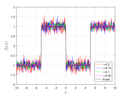
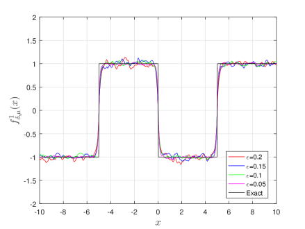
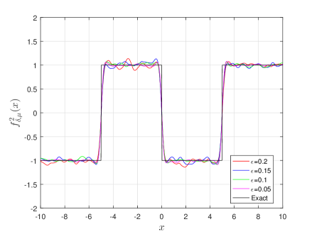
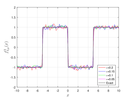
The table 1 includes the relative estimation errors that also show the goodness of the methods used. As noted, for this example, the operator performs better. For example, for the case , the relative error of the estimate of the regularized source with is , with is and with it is .
| Relative errors | ||||||||||||||||||||||||
|
Example 2.
For this example, the following parameters are considered ; ; 0; and . Furthermore, the perturbation values used are 0.001}. Finally, the source to estimate in this case is:
| (48) |
The source (48) recovered in example 2 is of interest in heat transfer problems. See for example, [53]. This type of function turns out to be a common example in source recovery problems in heat transfer processes [48, 50]. The example 2 is interesting, since this type of sources have already been recovered by means of different approaches in simpler problems where it is used, instead of the full parabolic equation, the heat equation where only diffusion is taken into account [32, 34, 35].
Table 2 includes the relative estimation errors that also show the goodness of the methods used. As noted, for this example, the operator performs better. For example, for the case , the relative error of the estimate of the regularized source with is , with is and with it is .
As it can be seen in the graphs of figure 2, the regularization operators used, again, smooth the inverse operator making the recovery stable. In this case, the stabilization effect is much more noticeable to the naked eye (because smaller values of disturbances were considered); due to this and for comparative purposes, a smaller scale was taken for the sources retrieved with the regularization operators. Once again it can be seen that the estimation improves for smaller values of disturbance . Also, no significant differences between the different operators are noticeable to the naked eye, although the operator seems to have, in this example, a better overall performance.
| Relative errors | ||||||||||||||||||||||||
|
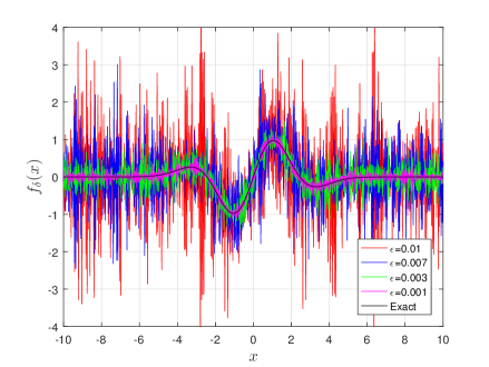
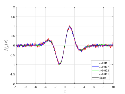
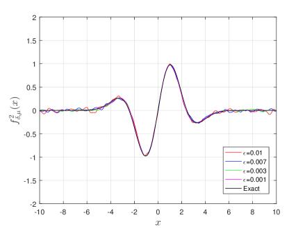
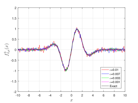
Example 3.
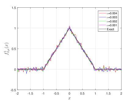
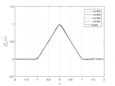
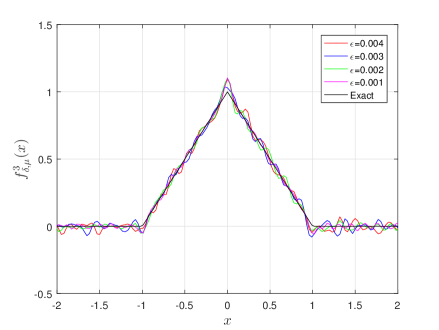
For this example, the following parameters are considered ; ; ; and . Furthermore, the perturbation values used are 0.0001}. Finally, the source to estimate in this case is:
| (49) |
The source (49) that is recovered in the example 3 is of interest in various problems with different characteristics due to the particularities that this function presents. Although it is a continuous function, it has a point where it is not differentiable. Recovery is often difficult at these points. Because of this, this type of function also turns out to be a common example in source recovery problems, both in signal theory and in heat transfer problems [48, 50].
Table 3 includes the relative estimation errors that again show the benefits of using the methods presented in this article. As noted, for this example, the operator performs better. For example, for the case , the relative error of the estimate of the regularized source with is , with is and with it is .
| Relative errors | ||||||||||||||||||||||||
|
As can be seen in the graphs of figure3, the regularization operators used, again, smooth the inverse operator making the recovery stable. In this case the stabilization effect, too, is more noticeable to the naked eye than in the example 1. This is because small values of perturbations were considered in order to be able to compare the regularization solutions with the non-regularized ones (which, again, presented many fluctuations). Due to this reason and for comparative purposes, a smaller scale was taken for the sources retrieved with the regularization operators. Once again it can be seen that the estimation improves for smaller values of disturbance . Furthermore, no significant differences between the different operators are noticeable to the naked eye, although the operator clearly provides a better estimate.
3.3.2 Examples 2D
Here are two examples of two-dimensional estimation with different characteristics. In order to visualize more clearly the improvements obtained with the regularization operators, not only the recovered sources will be graphed, but also contour lines will be made. These schemes will allow direct comparisons to be made on the sources obtained with the different regularization strategies.
Example 4.
For this example, the following parameters are considered ; ; ; ; and . Finally, the source to estimate in this case is:
| (50) |
The source (50) that is recovered in the example 4 is of interest in various problems with different characteristics due to the particularities that this function presents. Its graph is a surface, smooth, continuous and differentiable.
As can be seen in the graphs of figure 4, the regularization operators used, again, smooth the inverse operator making the recovery stable. No significant differences between the different operators are noticeable with the naked eye, although if the level curves are visualized and compared, the operator provides a better estimate.
Table 4 includes the relative estimation errors that once again show the good performance obtained with the methods introduced in this article. As noted, for this example, the operator performs better overall. For example, for the case , the relative error of the estimate of the source regularized with is , with is and with it is .
| Relative errors | ||||||||||||||||||||||||
|
Example 5.
For this example, the following parameters are considered ; ; ; ; and . Finally, the source to estimate in this case is:
| (51) |
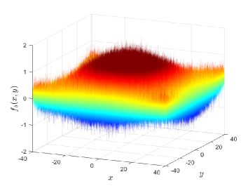
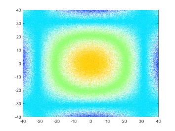

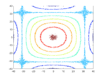
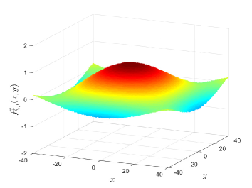
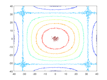
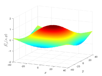
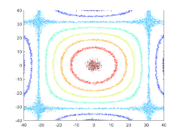
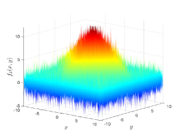
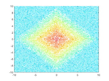

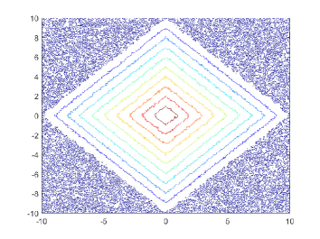
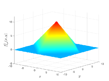
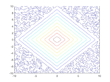
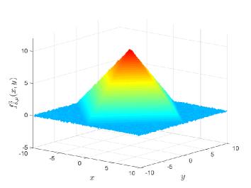
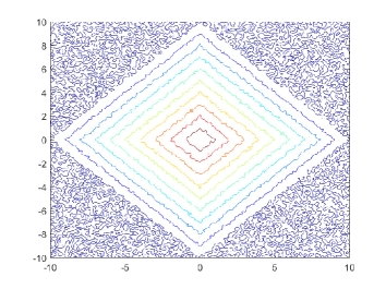
The source (51) retrieved in example 5 is of interest because it is a non-differentiable surface. This type of surfaces can be approximated badly in environments close to the points of non-differentiability.
As can be seen in the graphs of figure 5, once again, the regularization operators used, smooth the inverse operator making the recovery stable. No significant differences between the different operators are noticeable at first glance, although if the level curves are visualized and compared, once again, the operator provides a better estimate, more effectively stabilizing the solution of the ill-posed problem.
Table 5 includes the relative estimation errors that once again show the good performance obtained with the methods introduced in this paper. As observed, for this example, the operator presents a better general performance, since it achieves a better stabilization of the solution. For example, for the case , the relative error of the estimate of the regularized source with is , with is and with it is .
| Relative errors | ||||||||||||||||||||||||
|
3.3.3 Examples 3D
An example of three-dimensional estimation is now addressed. Since in this case the source is a scalar function with domain in , 4 dimensions are required to be able to plot it, because of this, only the cuts with the coordinate axes will be plotted. That is, the graphs of the retrieved sources will be analyzed when one of the variables is null. In addition, to visualize more clearly the improvements obtained with the different regularization operators introduced and studied in this article, contour diagrams will be made for each of the cuts considered and for each regularization.
Example 6.
For this example, the following parameters are considered ; ; ; ; and . Finally, the source to estimate in this case is:
| (52) |
The source (52) that is recovered in the example 6 is of interest in various problems with different characteristics due to the particularities that this function presents. It is a function, smooth, continuous and differentiable; moreover, it is symmetric with respect to the three coordinates.
| Relative errors | ||||||||||||||||||||||||
|
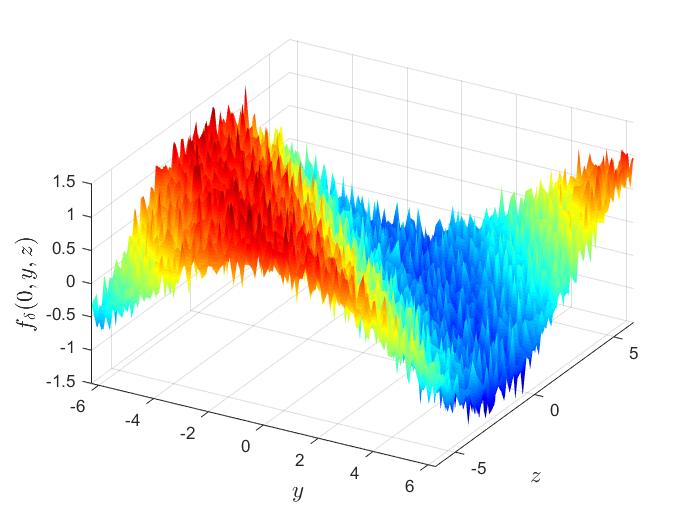
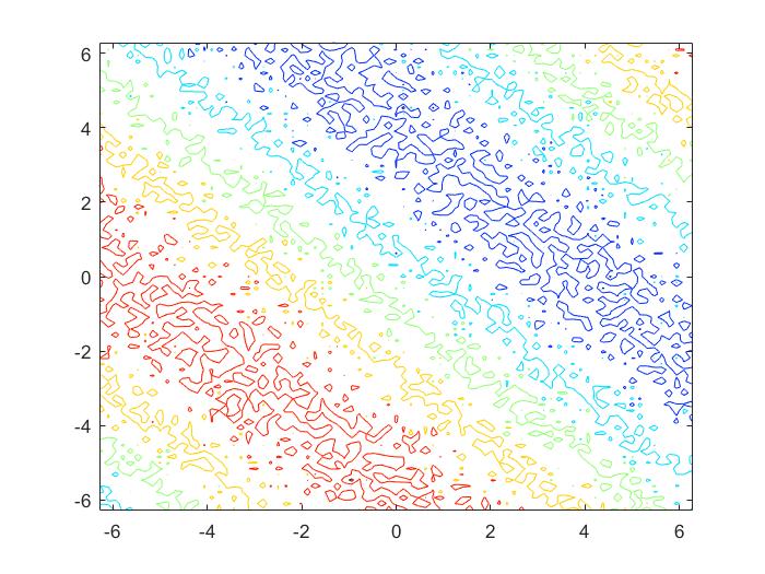

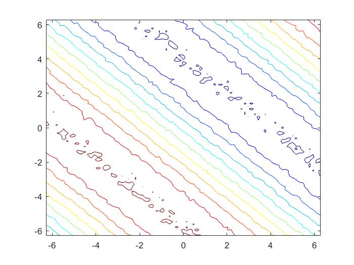

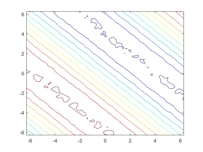
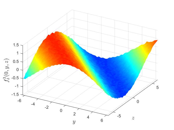
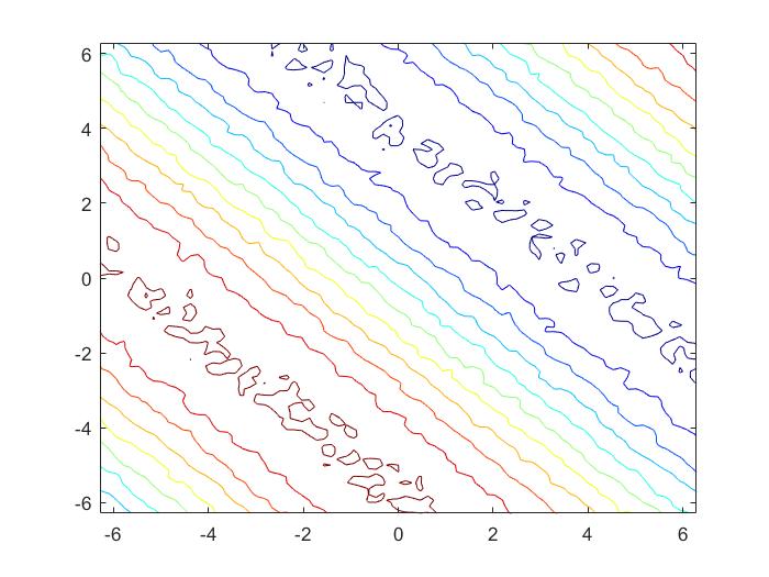
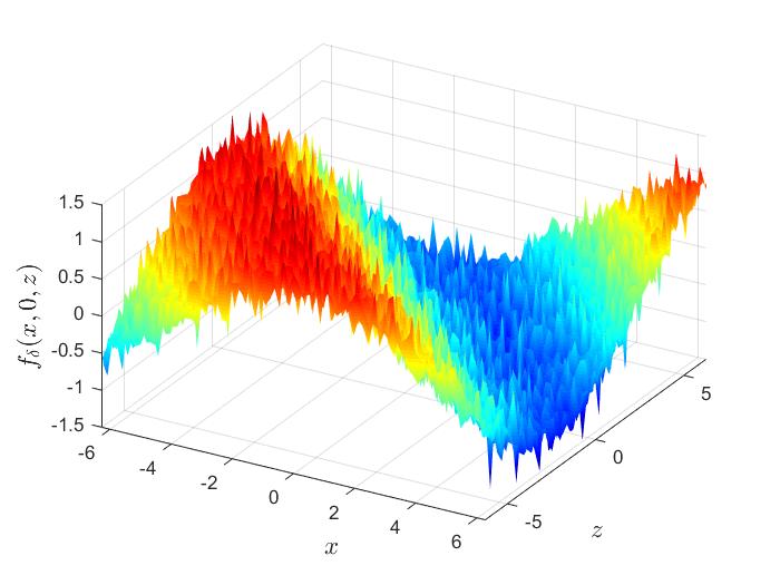
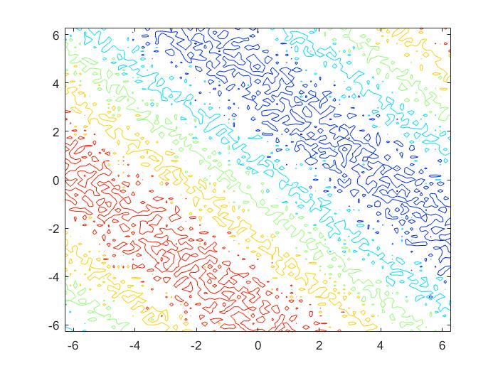

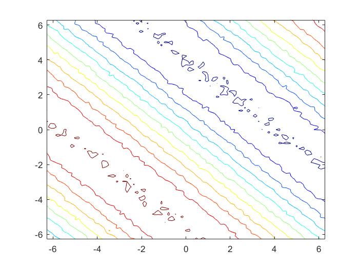

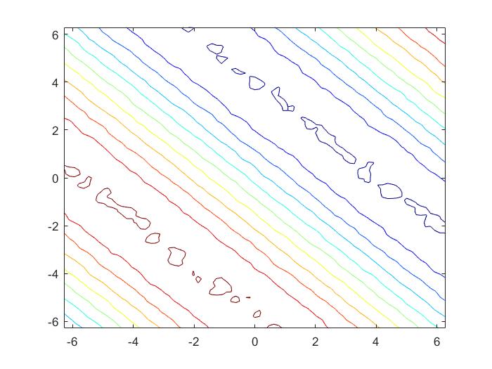
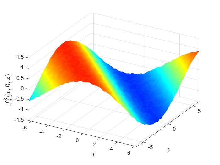
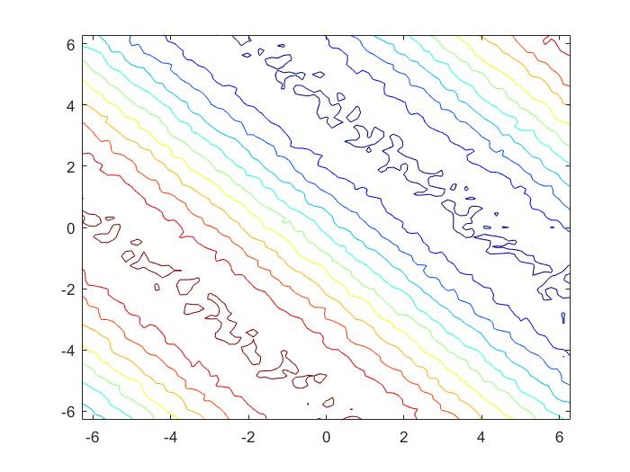
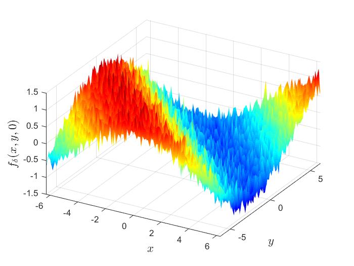
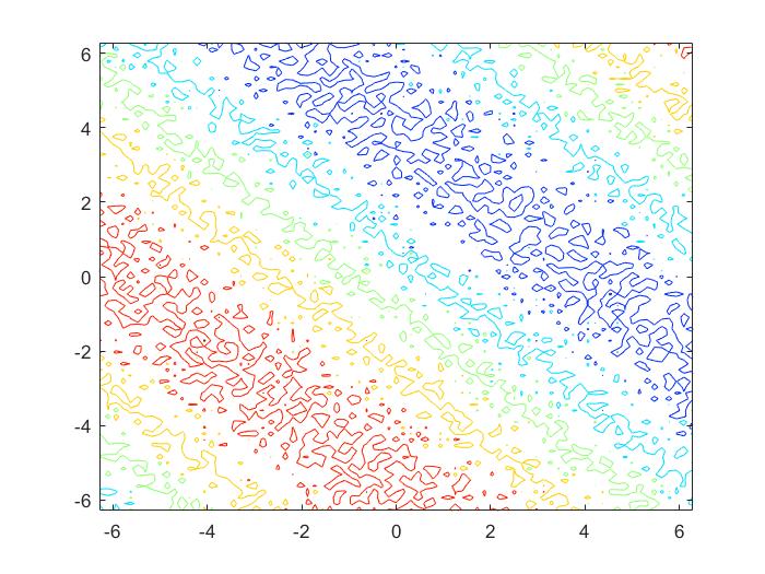

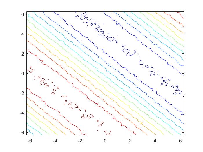

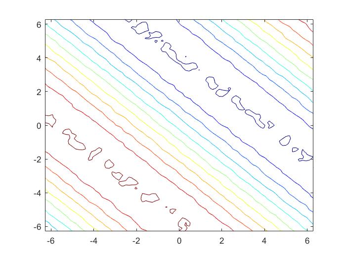

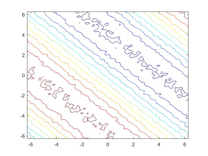
Table 6 includes the relative estimation errors that once again show the good performance obtained with the methods introduced in this article. As noted, in this example, the operator performs better overall. For example, for the case , the relative error of the estimate of the regularized source with is , with is and with it is .
As can be seen in the graphs of the figures 6, 7, 8 the regularization operators used, again, smooth the inverse operator making the recovery in each cut with the coordinate axes stable. In principle, notable differences between the recovery of each cut are not appreciated; since they are all estimated with the same order of fluctuation. On the other hand, no significant differences between the approximations with the different regularization operators are noticeable at first glance. If the level curves are carefully observed, for each cut with the coordinate axes, it is seen that, once again, the operator yields better results.
3.4 Discussion of results
The numerical examples carried out show that the three regularization operators, introduced in this article, are useful to solve the problem of lack of stability in the source estimation solution. Any of the three operators studied smooth out the inverse operator making the recovery stable. This fact is independent of the general characteristics of the function to be determined, since the results are good, even for discontinuous and non-differentiable sources.
However, in general terms the operator yielded better results and allowed estimating the source with the lowest relative error, for the different disturbances considered. Particularly the operator offered a better performance when the source to be estimated is a discontinuous function.
4 Conclusions
This paper deals with the inverse problem of identifying the source in a complete parabolic equation from noisy measurements. An analytical solution to the estimation problem is given and shown that the problem is ill-posed since said solution is not stable. In order to address this drawback, three families of regularization operators specifically designed to compensate for the instability factor in the inverse operator are defined. Besides, a choice rule is included for the regularization parameters that is based on the level of data noise and the smoothness of the source to be identified. It is shown that for the proposed parameter choice rule the methods are stable. A bound is obtained for the estimation errors that turn out to be optimal since they are of Hölder type.
Several numerical examples of recovering sources that belong to different spaces of Hilbert are included. It is observed that in all of them a good performance of the adopted regularization approaches is obtained. On the other hand, the sources recovered by means of the inverse operator are compared with those obtained using the regularization operators and it is concluded that the proposed regularization methods offer greater precision in the estimation of the sources considered.
References:
-
[1]
R. Bird, Transport phenomena. Wiley, New York (2002).
https://doi.org/10.1115/1.1424298
-
[2]
K. Hangos, I. Cameron, Process modelling and model analysis. Academic Press, Cambridge (2001).
https://doi.org/10.1016/s1874-5970(01)x8001-6
-
[3]
G.F. Umbricht, D. Rubio, C. El Hasi, Solución analítica de un problema de transferencia de energía térmica con generación de calor, disipación por convección y flujo lateral. Matemática Aplicada, Computacional e Industrial 8 (2021), pp. 679–682.
https://asamaci.org.ar/wp-content/uploads/2021/07/MACI-Vol-8-2021.pdf
-
[4]
H. Pennes, Analysis of tissue and arterial blood temperature in the resting human forearm. Journal of Applied Physiology 1(2) (1948), pp. 93–122.
http://dx.doi.org/10.1152/jappl.1948.1.2.93
-
[5]
H.A. Basha, F.S. El Habel, Analytical solution of the one-dimensional time-dependent transport equation. Water Resources Research 29(9) (1993), pp. 3209–3214.
https://doi.org/10.1029/93WR01038
-
[6]
O.M. Alifanov, F.A. Artyukhin, Regularized numerical solution of nonlinear inverse heat conduction problem. Journal of Engineering Physics and Thermophysics 29(1) (1975), pp. 934–938.
https://doi.org/10.1007/bf00860643
-
[7]
L. Eldén, F. Berntsson, T. Reginska, Wavelet and Fourier methods for solving the sideways heat equation. SIAM Journal on Scientific Computing 21(6) (2000), pp. 2187–2205.
http://dx.doi.org/10.1137/S1064827597331394
-
[8]
G.F. Umbricht, Estimación de la fuente en una ecuación de Poisson: mediante un método de regularización. Editorial Académica Española, Riga, Letonia, Unión Europea (2019).
-
[9]
Z. Zhao, Z. Meng, A modified Tikhonov regularization method for a backward heat equation. Inverse Problems in Science and Engineering 19(8) (2011), pp. 1175–1182.
https://doi.org/10.1080/17415977.2011.605885
-
[10]
Y. Zeng, J.G. Anderson, A composite source model of the 1994 Northridge earthquake using genetic algorithms. Bulletin of the Seismological Society of America 86(1B) (1996), pp. S71–S83.
-
[11]
H.T. Banks, D. Rubio, N. Saintier, M.I. Troparevsky, Optimal design for parameter estimation in EEG problems in a 3D multilayered domain. Mathematical Biosciences and Engineering 12(4) (2015), pp. 739–760.
https://doi.org/10.3934/mbe.2015.12.739
-
[12]
P.Jr. Ciaret, F. Lefèvre, S. Lohrengel, S. Nicaise, Weighted regularization for composite materials in electromagnetism. ESAIM: Mathematical Modelling and Numerical Analysis 44 (2010), pp. 75–108.
https://doi.org/10.1051/m2an/2009041
-
[13]
A. El Badia, T. Ha-Duong, An inverse source problem in potential analysis. Inverse Problems 16(3) (2000), pp. 651–663.
https://doi.org/10.1088/0266-5611/16/3/308
-
[14]
G.C. Beroza, P. Spudich, Linearized inversion for fault rupture behavior: application to the 1984 Morgan Hill, California, earthquake. Journal of Geophysical Research: Solid Earth 93(B6) (1988), pp. 6275–6296.
https://doi.org/10.1029/JB093iB06p06275
-
[15]
G.S. Li, T.J. Tan, J. Cheng, X.Q. Wang Determining magnitude of groundwater pollution sources by data compatibility analysis. Inverse Problems in Science and Engineering 14(3) (2006), pp. 287–300.
http://dx.doi.org/10.1080/17415970500485153
-
[16]
R. Macleod, W.G. Dirks, Y. Matsuo, M. Kaufmann, H. Milch, H.G. Drexler Widespread intraspecies cross-contamination of human tumor cell lines arising at source. International Journal of Cancer 83(4) (1999), pp. 555–563.
http://dx.doi.org/10.1002/(SICI)1097-0215(19991112)83:4%3C555::AID-IJC19%3E3.0.CO;2-2
-
[17]
T. Ohe, K. Ohnaka, A precise estimation method for locations in an inverse logarithmic potential problem for point mass models. Applied Mathematical Modelling 18(8) (1994), pp. 446–452.
http://dx.doi.org/10.1016/0307-904X(94)90306-9
-
[18]
T. Nara, S. Ando, A projective method for an inverse source problem of the Poisson equation. Inverse Problems 19(2) (2003), pp. 355–369.
http://dx.doi.org/10.1088/0266-5611/19/2/307
-
[19]
Y.C. Hon, M. Li, Y.A. Melnikov, Inverse source identification by Green’s function. Engineering Analysis with Boundary Elements 34(4) (2010), pp. 352–358.
http://dx.doi.org/10.1016/j.enganabound.2009.09.009
-
[20]
A. Farcas, L. Elliott, D.B. Ingham, D. Lesnic, S. Mera, A dual reciprocity boundary element method for the regularized numerical solution of the inverse source problem associated to the Poisson equation. Inverse Problems in Engineering 11(2) (2003), pp. 123–139.
http://dx.doi.org/10.1080/1068276031000074267
-
[21]
Y. Sun, Y. kagawa, Identification of electric charge distribution using dual reciprocity boundary element models. IEEE Transactions on Magnetics 33(2) (1997), pp. 1970–1973.
http://dx.doi.org/10.1109/20.582682
-
[22]
B. Jin, L. Marin, The method of fundamental solutions for inverse source problems associated with the steady-state heat conduction. International Journal for Numerical Methods in Engineering 69(8) (2007), pp. 1570–1589.
http://dx.doi.org/10.1002/nme.1826
-
[23]
G.F. Umbricht, D. Rubio, C. El Hasi, A regularization operator for the source approximation of a transport equation. Mecánica Computacional 37(50) (2019), pp. 1993–2002.
https://cimec.org.ar/ojs/index.php/mc/article/view/6032
-
[24]
G.F. Umbricht, D. Rubio, Identificación de la fuente en una ecuación de transferencia de calor en un tejido biológico. Matemática Aplicada, Computacional e Industrial 7 (2019), pp. 405–408.
https://asamaci.org.ar/wp-content/uploads/2021/06/MACI-Vol-7-2019.pdf
-
[25]
G.F. Umbricht, Identification of the source for full parabolic equation. Mathematical Modelling and Analysis 26(3) (2021), pp: 339–357.
https://doi.org/10.3846/mma.2021.12700
-
[26]
A. Farcas, D. Lesnic, The boundary-element method for the determination of a heat source dependent on one variable. Journal of Engineering Mathematics 54(4) (2006), pp. 375–388.
http://dx.doi.org/10.1007/s10665-005-9023-0
-
[27]
M. Ahmadabadi, M. Arab, F.M. Maalek Ghaini, The method of fundamental solutions for the inverse space-dependent heat source problem. Engineering Analysis with Boundary Elements 33(10) (2009), pp. 1231–1235.
https://doi.org/10.1016/j.enganabound.2009.05.001
-
[28]
B.T. Johansson, D. Lescnic, Determination of a spacewise dependent heat source. Journal of Computational and Applied Mathematics 209(1) (2007), pp. 66–80.
http://dx.doi.org/10.1016/j.cam.2006.10.026
-
[29]
C.S. Liu, An two-stage LGSM to identify time dependent heat source through an internal measurement of temperature. International Journal of Heat and Mass Transfer 52(7–8) (2009), pp. 1635–1642.
http://dx.doi.org/10.1016/j.ijheatmasstransfer.2008.09.021
-
[30]
E.G. Savateev, On problems of determining the source function in a parabolic equation. Journal of Inverse and Ill-posed Problems 3(1) (1995), pp. 83–102.
http://dx.doi.org/10.1515/jiip.1995.3.1.83
-
[31]
J.R. Cannon, P. Duchateau, Structural identification of an unknown source term in a heat equation. Inverse Problems 14(3) (1998), pp. 535–551.
http://dx.doi.org/10.1088/0266-5611/14/3/010
-
[32]
L. Yan, C.L. Fu, F.L. Yang, The method of fundamental solutions for the inverse heat source problem. Engineering Analysis with Boundary Elements 32(3) (2008), pp. 216–222.
http://dx.doi.org/10.1016/j.enganabound.2007.08.002
-
[33]
K. Rashedi, S.A. Yousef, Ritz-Galerkin Method for solving a class of inverse problems in the parabolic equation. International Journal of Nonlinear Science 12(4) (2011), pp. 498–502.
http://citeseerx.ist.psu.edu/viewdoc/download?doi=10.1.1.1086.9901&rep=rep1&type=pdf
-
[34]
L. Yan, C.L. Fu, F.F. Dou, A computational method for identifying a spacewise-dependent heat source. International Journal for Numerical Methods in Biomedical Engineering 26(5) (2010), pp. 597–608.
https://doi.org/10.1002/cnm.1155
-
[35]
L. Yan, F.L. Yang, C.L. Fu, A meshless method for solving an inverse spacewise-dependent heat source problem. Journal of Computational Physics 228(1) (2009), pp. 123–136.
https://doi.org/10.1016/j.jcp.2008.09.001
-
[36]
M. Yamamoto, Conditional stability in determination of force terms of heat equations in a rectangle. Mathematical and Computer Modelling 18(1) (1993), pp. 79–88.
http://dx.doi.org/10.1016/0895-7177(93)90081-9
-
[37]
J. Hadamard, Lectures on Cauchy’s problem in linear partial differential equations. The Mathematical Gazette 12(171) (1924), pp. 173–174.
https://doi.org/10.2307/3603014
-
[38]
H.W. Engl, M. Hanke, A. Neubauer, Regularization of Inverse Problems. Kluwer Academic, Boston (1996).
https://www.springer.com/gp/book/9780792341574
-
[39]
A. Kirsch, An introduction to the mathematical theory of inverse problems. Springer, New York (2011).
http://dx.doi.org/10.1007/978-1-4419-8474-6
-
[40]
M. Hochbruck, M. Hönig, A. Ostermann, Regularization of nonlinear ill-posed problems by exponential integrators. ESAIM: Mathematical Modelling and Numerical Analysis 43 (2009), pp. 709–720.
https://doi.org/10.1051/m2an/2009041
-
[41]
B.T. Johansson, D. Lescnic, A procedure for determining a spacewise dependent heat source and the initial temperature. Applicable Analysis: An International Journal 87(3) (2008), pp. 265–276.
http://dx.doi.org/10.1080/00036810701858193
-
[42]
C.L. Fu, Simplified Tikhonov and Fourier regularization methods on a general sideways parabolic equation. Journal of Computational and Applied Mathematics 167(2) (2004), pp. 449–463.
http://dx.doi.org/10.1016/j.cam.2003.10.011
-
[43]
W. Cheng, C.L. Fu, Z. Quian, A modified Tikhonov regularization method for a spherically symmetric three-dimensional inverse heat conduction problem. Mathematics and Computers in Simulation 75(3–4) (2007), pp. 97–112.
http://dx.doi.org/10.1016/j.matcom.2006.09.005
-
[44]
W. Cheng, C.L. Fu, Z. Quian, Two regularization methods for a spherically symmetric inverse heat conduction problem. Applied Mathematical Modelling 32(4) (2008), pp. 432–442.
http://dx.doi.org/10.1016/j.apm.2006.12.012
-
[45]
F. Natterer, Error bounds for Tikhonov regularization in Hilbert scales. Applicable Analysis: An International Journal 18(1–2) (1984), pp. 29–37.
http://dx.doi.org/10.1080/00036818408839508
-
[46]
F. Yang, C.L. Fu, A simplified Tikhonov regularization method for the heat source. Applied Mathematical Modelling 34(11) (2010), pp. 3286–3299.
http://dx.doi.org/10.1016/j.apm.2010.02.020
-
[47]
F. Yang, C.L. Fu, The method of simplified Tikhonov regularization for dealing with the inverse time-dependent heat source problem. Computers and Mathematics with Applications 60(5) (2010), pp. 1228–1236.
http://dx.doi.org/10.1016/j.camwa.2010.06.004
-
[48]
F. Yang, C.L. Fu, Two regularization methods to identify time-dependent heat source through an internal measurement of temperature. Mathematical and Computer Modelling 53(5–6) (2011), pp. 793–804.
http://dx.doi.org/10.1016/j.mcm.2010.10.016
-
[49]
Z. Zhao, O. Xie, Z. Meng, L. You, Determination of an unknown source in the heat equation by the method of Tikhonov regularization in Hilbert scales. Journal of Applied Mathematics and Physics 2(2) (2014), pp. 10–17.
http://dx.doi.org/10.4236/jamp.2014.22002
-
[50]
F. Yang, C.L. Fu, A mollification regularization method for the inverse spatial-dependent heat source problem. Journal of Computational and Applied Mathematics 255(C) (2014), pp. 555–567.
http://dx.doi.org/10.1016/j.cam.2013.06.012
-
[51]
I.F. Sivergina, M.P. Polis, I. Kolmanovsky, Source identification for parabolic equations. Mathematics of Control, Signals, and Systems 16(2–3) (2003), pp. 141–157.
http://dx.doi.org/10.1007/s00498-003-0136-6
-
[52]
F.F Dou, C.L. Fu, Determining an unknown source in the heat equation by a wavelet dual least squares method. Applied Mathematics Letters 22(5) (2009), pp. 661–667.
http://dx.doi.org/10.1016/j.aml.2008.08.003
-
[53]
F.F. Dou, C.L. Fu, F.L. Yang, Optimal error bound and Fourier regularization for identifying an unknown source in the heat equation. Journal of Computational and Applied Mathematics 230(2) (2009), pp. 728–737.
http://dx.doi.org/10.1016/j.cam.2009.01.008
-
[54]
T.J. Martin, G.S. Dulikravich, Inverse determination of boundary conditions and sources in steady heat conduction with heat generation. Journal of Heat Transfer 118(3) (1996), pp. 546–554.
http://dx.doi.org/10.1115/1.2822666
-
[55]
D.D. Trong, N.T. Long, P.N.D. Alain, Nonhomogeneous heat equation: identification and regularization for the inhomogeneous term. Journal of Mathematical Analysis and Applications 312(1) (2005), pp. 93–104.
http://dx.doi.org/10.1016/j.jmaa.2005.03.037
-
[56]
D.D. Trong, P.H. Quan, P.N.D. Alain, Determination of a two-dimensional heat source: uniqueness, regularization and error estimate. Journal of Computational and Applied Mathematics 191(1) (2006), pp. 50–67.
http://dx.doi.org/10.1016/j.cam.2005.04.022
-
[57]
Q. Li, L.H. Nguyen, Recovering the initial condition of parabolic equations from lateral Cauchy data via the quasi-reversibility method. Inverse Problems in Science and Engineering 28(4) (2020), pp. 580–598.
https://doi.org/10.1080/17415977.2019.1643850
-
[58]
T.T. Le, L.H. Nguyen, A convergent numerical method to recover the initial condition of nonlinear parabolic equations from lateral cauchy data. Journal of Inverse and Ill-posed Problems 14(3) (2020), pp. 287–300.
https://doi.org/10.1515/jiip-2020-0028
- [59] P. Das, S. Begam, M.K. Singh, Mathematical modeling of groundwater contamination with varying velocity field. Journal of Hydrology and Hydromechanics 65(2) (2017), pp. 192–204. https://doi.org/10.1515/johh-2017-0013
-
[60]
N.Z. Sun, A. Sun, Mathematical modeling of groundwater pollution. Springer, New York (1996).
https://www.springer.com/gp/book/9781475725605
-
[61]
R.J. Marks, Handbook of Fourier analysis & its applications. Oxford university press, New York (2009).
https://doi.org/10.1093/oso/9780195335927.001.0001
-
[62]
C. Van Loan, Computational frameworks for the fast Fourier transform. SIAM, Philadelphia (1992).
http://dx.doi.org/10.1137/1.9781611970999