spacing=nonfrench
Quantum non-classicality in the simplest causal network
Abstract
Bell’s theorem prompts us with a fundamental inquiry: what is the simplest scenario leading to the incompatibility between quantum correlations and the classical theory of causality? Here we demonstrate that quantum non-classicality is possible in a network consisting of only three dichotomic variables, without the need of the locality assumption neither external measurement choices. We also show that the use of interventions, a central tool in the field of causal inference, significantly improves the noise robustness of this new kind of non-classical behaviour, making it feasible for experimental tests with current technology.
Introduction.— Bell’s theorem [1] is often considered the most stringent notion of non-classicality. Based solely on the causal assumptions of locality and freedom of choice one can exclude any physical theories based on presumption that a hidden variable can predetermine the properties and measurement outcomes of entangled systems. Given its far reaching foundational consequences and application for information processing [2], it is natural to question whether non-classical behaviour can emerge even if we give up or relax some of these assumptions. After all, while historically essential, when seen from the lens of causality theory [3], Bell’s theorem is just one example of a causal compatibility problem [4, 5, 6], the aim of which is to decide a given experimental data can be generated by an underlying causal structure or not.
Within this new perspective, there are many physically motivated causal structures beyond Bell’s and the recent years have seen an increasing interest in understanding the non-classical behaviour and applications they can lead to. In these generalizations, two new ingredients, relaxations of the causal assumptions in Bell’s theorem, emerge as essential. Firstly, correlations between distant parties can be mediated by independent sources, a common occurrence in network scenarios [7] and that can lead to scenarios without the need of the freedom of choice [8, 9, 10, 11, 12]. Secondly, time-like correlations come to the fore, where the choices and outcomes of measurements by one observer directly influence another [13, 14]. The independence of sources in networks have revealed new features such as the need of complex numbers in quantum theory [15], refined forms of multipartite non-locality [16, 17, 18] and the self-testing of physical theories [19]. In turn, scenarios with communication have led to new witness of non-classicality based on interventions and the violation of causal bounds [20, 21, 22, 23]. The combination of both features, source independence and communication in network scenarios, however, are mostly unexplored.
The simplest network combining both ingredients, known as the Unrelated Confounders (UC) scenario [24, 25], is displayed in Fig. 1(c) and can be understood as the causal structure underpinning an entanglement swapping experiment [26]. Similarly to the triangle causal structure [8, 9] displayed in Fig. 1(b), this new scenario involves independent sources and does not require the need of external inputs. In turn, similarly to the instrumental scenario [27, 13] displayed in Fig. 1(a), it incorporates direct causal influences between the observable nodes. And while it is known that quantum correlations are incompatible with both the instrumental [13, 28] and triangle [8, 9] causal assumptions, it remains an open question whether the same holds for the UC case [25, 29]. This is the problem we solve here, showing that quantum correlations incompatible with a classical description of the UC scenario can indeed emerge. Interestingly, quantum violations are possible even in the simplest case, where all measurements are dichotomic, which remains an important open problem in other networks such as the triangle [30, 31]. Furthermore, we show how the use of interventional data [21] can significantly increase the noise robustness, turning the Unrelated Confounders scenario into the most experimentally feasible network displaying a novel form of non-classicality beyond that in the paradigmatic Bell experiment.
Unrelated Confounders Scenario—The UC scenario [24, 25] is the underlying causal structure (see Fig. 1(c)) for a pivotal protocol in quantum information science known as entanglement swapping [26]: a central node, Bob, shares independent entangled states with the uncorrelated nodes of Alice and Charlie; if Bob performs an entangled measurement and communicates its outcomes then Alice and Charlie can also become entangled. It features three observed variables , , and for the outcomes of Alice, Bob, and Charlie respectively. And independent sources of correlation between and between , such that . Classically, observations compatible with such causal structure factorize as
| (1) |
For quantum theory, we have the sources distributing quantum information; the global state is and the POVMs describing the measurements on it are given by , and . Born’s rule implies then that the observed probabilities obtained when we impose the UC causal structure to a given experiment are given by
| (2) |
Importantly, the presence of communication of the output of to and , allows us to go beyond passive observations of the experiment and investigate the role of interventions [32, 3]. In contrast to observations, interventions allow to locally change the causal structure, eliminating all external influences of a given variable , forcing it to a particular value while keeping the rest of the model unchanged. Classically, an intervention in node of the UC scenario (see Fig. 1(d)) breaks the correlations between nodes and , defining a do-conditional given by
| (3) |
where and similarly for . In turn, if the sources distribute quantum states the do-conditional still respects (3), with
| (4) |
and similarly for .
Concave inequalities— Causal networks with independent sources, as is the case in the UC scenario, have a non-convex set of correlations [33] described by polynomial Bell inequalities [34] that can be significantly difficult to be characterized [6, 35, 36]. Given that general techniques such as inflation are known to perform poorly on the UC case [29], we show next how one can leverage quadratic programming (QP) [37] to circumvent these issues and derive useful data-driven and robust non-linear witness for non-classicality.
Given the independence of the two sources represented by the quadratic constraint , the corresponding Bell inequalities should also be quadratic, being expressed equivalently by a functional depending square root of the probability of the experiment [38, 39, 34]. To further restrict the set of classical correlations in the UC network, we can also add penalty functions that force the inequality we are looking at to a subspace of the set of allowed correlations. For instance, suppose that in a given experiment we observe that the marginal distribution of Bob outcomes respect . Adding a term like to the inequality, we construct a witness tailored to that specific observed correlation. Thus, in the following, we will focus on inequalities with the following functional form
| (5) |
where and are linear functions of .
Given a certain expression of the form (5), our aim is to find its maximum value in a classical description of causality and further search for quantum violations of it. Even though we are thus dealing with a nonconvex optimization problem, The general framework of linear programming (LP) [40] can still be quite versatile and useful for our purposes. For instace, we can optimize expressions like by defining a new variable with the constraints and . Minimizing ultimately yields the same result as minimizing . Going beyond the linear programming and convex optimization paradigm, we can turn to quadratic optimization [37] to incorporate expressions of the form , with , by defining a new variable and adding the restriction which can easily be imposed in a quadratic program. With that, we can reformulate an optimization of the general expression (5) into
| (6) | ||||
which is a typical instance of quadratic programming [37].
As will be shown in the following, in order to reveal the non-classicality in the UC it is enough to consider its simplest version where all observable variables are binary. Also, we notice that has access to all the information from the sources and . Then by sending its output to the remaining parts, it can effectively send information from to and, similarly, from to . However, this forwarding of information is limited by the cardinality of . This suggests to look at the correlation between and for each value of . For simplicity, we use correlators as auxiliary variables. Defining , and we have
| (7) |
with an inverse map given by
| (8) |
Following the intuition delineated above, we will see that the following non-linear function
| (9) | ||||
provides a good witness of non-classicality in the UC scenario. Using a standard QP optimizer [41], we observe that the classical causal model (1) respects . 111We obtain this classical upper bound using QP with a precision of .
Following the same reasoning, we can add terms to the inequality that incorporate interventional data, that is, adding terms that depend on and into the inequality. A particularly useful function is given by
| (10) | ||||
Optimizing it using QP under the classical constraints given by (1) and (3) we obtain .
Quantum non-classicality— To prove the emergence of non-classicality, we consider the following family of quantum distributions generated by a real parameter . Each of the two sources corresponds to the bipartite Bell state
| (11) |
and we take and to perform the binary measurements observables for and for . In turn performs the entangling measurement , where is given by
| (12) |
Using this quantum strategy, by direct computation we obtain
| (13) | ||||
with and and corresponding marginals given by
| (14) | ||||
This choice leads to a simplified form for the non-linear expression in inequality (9), expressed as
| (15) |
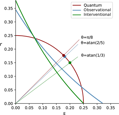
Choosing , i.e. by having measure in an incomplete and partially entangled Bell basis, we find , thus proving the existence of quantum non-classical correlations in the simplest non-trivial causal structure. The inequality (9) and the set of quantum correlations (13) are represented in Fig. 2.
To probe the robustness and experimental feasibility of this non-classicality, we consider a paradigmatic noise model that introduces isotropic noise with a visibility to the quantum sources, that is, each source is now given by . Unfortunately, the best critical visibility we could find below which the violation of (9) is no longer possible is significantly high, given by .
On the other hand, considering interventions and keeping the same set of measurements and states, one can reach values of . Moreover, in this case, the required visibility is significantly lower and one can obtain violation of the hybrid observational-interventional inequality (10) for visibilities down to , bringing the test of this new form of non-classicality within the reach of current technology (for a more in-depth analysis of the robustness to noise see appendix C).
Discussion.— The simplest causal networks that can potentially lead to quantum correlations without a classical explanation require at least three observable variables. Within this context, it is known that there are only three different classes of DAGs [24]: the instrumental [27, 13], the triangle [8, 9] and the unrelated confounders [25] causal scenarios, shown in Fig. 1. It was known that the first two can lead to quantum non-classicality [13, 8] and here we prove that the same holds true for UC. The relevance of it is two-fold. First, it proves that all three observable DAGs support a classical-quantum gap. Second, as we argue next, it provides an example of the simplest and yet stronger form of non-classical behavior to date.
The instrumental case partially relaxes the locality assumption in Bell’s theorem, since the measurement outcome of one observer can define the measurement basis for the other. However, one still has to employ an external random variable as an input and invoke the instrumentality assumption, that the measurement choice of one observer has no direct causal influence over the other. In turn, the triangle scenario allows for non-classicality without the need of external inputs. However, it requires a space-like separation between all three parties in the network.
The UC scenario we analyze here does not require any external input and at the same time provides a strong relaxation of the locality assumption, since one part explicitly communicates its measurement outcomes. Even more remarkable is the fact that quantum violations of classical constraints in this simplest causal structure are possible in the minimal case where all observable nodes are dichotomic, something that is not possible in the instrumental [43] case and is still an open problem for the triangle [30, 31].
The results we prove here allow for much more experimentally feasible tests of non-classicality in quantum networks. On one side, the quantum violation we reveal only requires two-outcome incomplete Bell state measurements, in stark contrast with known proposals for the triangle network [9, 30]. Furthermore, even though in the purely observational case the required visibilities for the two sources of entangled states are very high, they can be brought with interventions to values that are certainly amenable with current technologies, also showing the power of interventional data as a witness of non-classicality.
Since all three observable node networks can lead to quantum violations of causal constraints, a natural question is to understand how generic is quantum non-classicality. Does it happen in any non-trivial causal network? If not, what are the key ingredients for the emergence of non-classical behaviour? As previous results have shown and our present findings reinforce, locality and freedom of choice, unavoidable requirements in a standard Bell test, can be relaxed. Moving beyond the foundational aspects, a practical relevant direction is to investigate the quantum information processing capabilities of the UC network, from randomness certification [44] to cryptographic and communication protocols [45].
Acknowledgements
This work was supported by the Serrapilheira Institute (Grant No. Serra-1708-15763), the Simons Foundation (Grant Number 1023171, RC), São Paulo Research Foundation FAPESP (Grant No. 2022/03792-4) the Brazilian National Council for Scientific and Technological Development (CNPq) (INCT-IQ and Grant No 307295/2020-6).
References
- Bell [1964] J. S. Bell, On the einstein podolsky rosen paradox, Physics Physique Fizika 1, 195 (1964).
- Brunner et al. [2014] N. Brunner, D. Cavalcanti, S. Pironio, V. Scarani, and S. Wehner, Bell nonlocality, Reviews of modern physics 86, 419 (2014).
- Pearl [2009] J. Pearl, Causality (Cambridge university press, 2009).
- Wood and Spekkens [2015] C. J. Wood and R. W. Spekkens, The lesson of causal discovery algorithms for quantum correlations: causal explanations of bell-inequality violations require fine-tuning, New Journal of Physics 17, 033002 (2015).
- Chaves et al. [2015] R. Chaves, R. Kueng, J. B. Brask, and D. Gross, Unifying framework for relaxations of the causal assumptions in bell’s theorem, Physical review letters 114, 140403 (2015).
- Wolfe et al. [2019] E. Wolfe, R. W. Spekkens, and T. Fritz, The inflation technique for causal inference with latent variables, Journal of Causal Inference 7, 20170020 (2019).
- Tavakoli et al. [2022] A. Tavakoli, A. Pozas-Kerstjens, M.-X. Luo, and M.-O. Renou, Bell nonlocality in networks, Reports on Progress in Physics 85, 056001 (2022).
- Fritz [2012] T. Fritz, Beyond bell’s theorem: correlation scenarios, New Journal of Physics 14, 103001 (2012).
- Renou et al. [2019] M.-O. Renou, E. Bäumer, S. Boreiri, N. Brunner, N. Gisin, and S. Beigi, Genuine quantum nonlocality in the triangle network, Physical review letters 123, 140401 (2019).
- Šupić et al. [2020] I. Šupić, J.-D. Bancal, and N. Brunner, Quantum nonlocality in networks can be demonstrated with an arbitrarily small level of independence between the sources, Physical Review Letters 125, 240403 (2020).
- Chaves et al. [2021] R. Chaves, G. Moreno, E. Polino, D. Poderini, I. Agresti, A. Suprano, M. R. Barros, G. Carvacho, E. Wolfe, A. Canabarro, et al., Causal networks and freedom of choice in bell’s theorem, PRX Quantum 2, 040323 (2021).
- Polino et al. [2023] E. Polino, D. Poderini, G. Rodari, I. Agresti, A. Suprano, G. Carvacho, E. Wolfe, A. Canabarro, G. Moreno, G. Milani, et al., Experimental nonclassicality in a causal network without assuming freedom of choice, Nature Communications 14, 909 (2023).
- Chaves et al. [2018] R. Chaves, G. Carvacho, I. Agresti, V. Di Giulio, L. Aolita, S. Giacomini, and F. Sciarrino, Quantum violation of an instrumental test, Nature Physics 14, 291 (2018).
- Brask and Chaves [2017] J. B. Brask and R. Chaves, Bell scenarios with communication, Journal of Physics A: Mathematical and Theoretical 50, 094001 (2017).
- Renou et al. [2021] M.-O. Renou, D. Trillo, M. Weilenmann, T. P. Le, A. Tavakoli, N. Gisin, A. Acín, and M. Navascués, Quantum theory based on real numbers can be experimentally falsified, Nature 600, 625 (2021).
- Coiteux-Roy et al. [2021] X. Coiteux-Roy, E. Wolfe, and M.-O. Renou, No bipartite-nonlocal causal theory can explain nature’s correlations, Physical review letters 127, 200401 (2021).
- Suprano et al. [2022] A. Suprano, D. Poderini, E. Polino, I. Agresti, G. Carvacho, A. Canabarro, E. Wolfe, R. Chaves, and F. Sciarrino, Experimental genuine tripartite nonlocality in a quantum triangle network, PRX Quantum 3, 030342 (2022).
- Pozas-Kerstjens et al. [2022] A. Pozas-Kerstjens, N. Gisin, and A. Tavakoli, Full network nonlocality, Physical review letters 128, 010403 (2022).
- Weilenmann and Colbeck [2020] M. Weilenmann and R. Colbeck, Self-testing of physical theories, or, is quantum theory optimal with respect to some information-processing task?, Physical Review Letters 125, 060406 (2020).
- Ringbauer et al. [2016] M. Ringbauer, C. Giarmatzi, R. Chaves, F. Costa, A. G. White, and A. Fedrizzi, Experimental test of nonlocal causality, Science advances 2, e1600162 (2016).
- Gachechiladze et al. [2020] M. Gachechiladze, N. Miklin, and R. Chaves, Quantifying causal influences in the presence of a quantum common cause, Physical Review Letters 125, 230401 (2020).
- Agresti et al. [2022] I. Agresti, D. Poderini, B. Polacchi, N. Miklin, M. Gachechiladze, A. Suprano, E. Polino, G. Milani, G. Carvacho, R. Chaves, et al., Experimental test of quantum causal influences, Science advances 8, eabm1515 (2022).
- Poderini et al. [2024] D. Poderini, R. Nery, G. Moreno, S. Zamora, P. Lauand, and R. Chaves, Observational-interventional bell inequalities, arXiv preprint arXiv:2404.05015 (2024).
- Evans [2016] R. J. Evans, Graphs for margins of bayesian networks, Scandinavian Journal of Statistics 43, 625 (2016).
- Lauand et al. [2023] P. Lauand, D. Poderini, R. Nery, G. Moreno, L. Pollyceno, R. Rabelo, and R. Chaves, Witnessing nonclassicality in a causal structure with three observable variables, PRX Quantum 4, 020311 (2023).
- Zukowski et al. [1993] M. Zukowski, A. Zeilinger, M. Horne, and A. Ekert, ” event-ready-detectors” bell experiment via entanglement swapping., Physical Review Letters 71 (1993).
- Pearl [1995] J. Pearl, On the testability of causal models with latent and instrumental variables, in Proceedings of the Eleventh conference on Uncertainty in artificial intelligence (1995) pp. 435–443.
- Van Himbeeck et al. [2019] T. Van Himbeeck, J. B. Brask, S. Pironio, R. Ramanathan, A. B. Sainz, and E. Wolfe, Quantum violations in the instrumental scenario and their relations to the bell scenario, Quantum 3, 186 (2019).
- Camillo et al. [2024] G. Camillo, P. Lauand, D. Poderini, R. Rabelo, and R. Chaves, Estimating the volume of correlation sets in causal networks, Physical Review A 109, 012220 (2024).
- Boreiri et al. [2023] S. Boreiri, A. Girardin, B. Ulu, P. Lipka-Bartosik, N. Brunner, and P. Sekatski, Towards a minimal example of quantum nonlocality without inputs, Physical Review A 107, 062413 (2023).
- Pozas-Kerstjens et al. [2023] A. Pozas-Kerstjens, A. Girardin, T. Kriváchy, A. Tavakoli, and N. Gisin, Post-quantum nonlocality in the minimal triangle scenario, New Journal of Physics 25, 113037 (2023).
- Balke and Pearl [1997] A. Balke and J. Pearl, Bounds on treatment effects from studies with imperfect compliance, Journal of the American statistical Association 92, 1171 (1997).
- Garcia et al. [2005] L. D. Garcia, M. Stillman, and B. Sturmfels, Algebraic geometry of bayesian networks, Journal of Symbolic Computation 39, 331 (2005).
- Chaves [2016] R. Chaves, Polynomial bell inequalities, Physical review letters 116, 010402 (2016).
- Åberg et al. [2020] J. Åberg, R. Nery, C. Duarte, and R. Chaves, Semidefinite tests for quantum network topologies, Physical Review Letters 125, 110505 (2020).
- Wolfe et al. [2021] E. Wolfe, A. Pozas-Kerstjens, M. Grinberg, D. Rosset, A. Acín, and M. Navascués, Quantum inflation: A general approach to quantum causal compatibility, Physical Review X 11, 021043 (2021).
- Nocedal and Wright [2006] J. Nocedal and S. J. Wright, Quadratic programming, Numerical optimization , 448 (2006).
- Branciard et al. [2010] C. Branciard, N. Gisin, and S. Pironio, Characterizing the nonlocal correlations created via entanglement swapping, Physical review letters 104, 170401 (2010).
- Tavakoli et al. [2014] A. Tavakoli, P. Skrzypczyk, D. Cavalcanti, and A. Acín, Nonlocal correlations in the star-network configuration, Physical Review A 90, 062109 (2014).
- Boyd and Vandenberghe [2004] S. P. Boyd and L. Vandenberghe, Convex optimization (Cambridge university press, 2004).
- Gurobi Optimization, LLC [2022] Gurobi Optimization, LLC, Gurobi Optimizer Reference Manual (2022).
- Note [1] We obtain this classical upper bound using QP with a precision of .
- Henson et al. [2014] J. Henson, R. Lal, and M. F. Pusey, Theory-independent limits on correlations from generalized bayesian networks, New Journal of Physics 16, 113043 (2014).
- Sekatski et al. [2023] P. Sekatski, S. Boreiri, and N. Brunner, Partial self-testing and randomness certification in the triangle network, Physical Review Letters 131, 100201 (2023).
- Lee and Hoban [2018] C. M. Lee and M. J. Hoban, Towards device-independent information processing on general quantum networks, Physical review letters 120, 020504 (2018).
Appendix A Quadratic optimization problem
In the main text, we described in general terms how we can obtain a classical bound for inequality (9) and (10) by describing the problem as an instance of Quadratic Programming (QP) optimization. For completeness, we show here the explicit formulation of such QP problems. For the observational case, we have
| (16) | ||||
| s.t. | (17) |
where is the set of classical compatible distributions in the UC scenario, shown in (1). It is sufficient, in this last constraint, to consider that the source carries the information of how Alice responds to each of Bob’s outcomes and similarly for and Charlie. Therefore, we may take the sources to be of the form and with a stochastic response function for Bob and deterministic response functions and for Alice and Charlie respectively. This model yields
| (18) |
Similarly, for the interventional case, we have
| (19) | ||||
| s.t. | (20) |
where now the requirement of being in is imposed on both the interventional and observational distribution, that should be compatible with the UC scenario, that is, besides the constraints in (18) we also have:
| (21) |
The problems are manifestly quadratic and non-convex, both in their objective functions, as described in the main text, and in the constraints (18) and (21). Solving these problems gives us optimal values for and , which we then approximate from above to finally obtain the upper bounds presented in the main text:
| (22) | |||
| (23) |
Appendix B Optimal classical strategy
The solution of the QP described in the previous section, besides giving us a bound for and , also furnishes an optimal classical strategy that can saturate that value. In particular from the numerical solution we obtain the following classical model.
We consider to be bits and to saturate the classical bound of we may consider the distributions
| (24) | |||
| (25) |
Then for the response function of , we have for , and otherwise. This strategy reaches . Similarly, for the inequality , we can choose distributions
| (26) | |||
| (27) |
and for ,
| (28) | |||
| (29) | |||
| (30) | |||
| (31) |
and otherwise. This model will give the value , which can be taken as a lower bound.
Appendix C Maximum values and robustness of the quantum violation
In this section, we discuss in more detail the study of the robustness and maximal values of the quantum violation for and . We consider the same strategy delineated in the main text. We choose as observables for both A and C with and respectively, and we define the projector in B as with
| (32) |
And we consider noisy states for the two sources.
This strategy gives the following values for and :
| (33) | ||||
| (34) |
These quantities are maximized, for any fixed , by and respectively, which, for perfect visibility , gives and , slightly above the violations obtained with presented in the main text. From Eq. (33) and (34) we can also obtain the critical noise value after which we cannot have a quantum violation anymore, which is and for the observational and the interventional case respectively. Performing numeric optimization shows that, at least using bipartite 2-qubits states, these values are optimal for these inequalities.