Climbing over the potential barrier during inflation via null energy condition violation

Abstract

The violation of the null energy condition (NEC) may play a crucial role in enabling a scalar field to climb over high potential barriers, potentially significant in the very early universe. We propose a single-field model where the universe sequentially undergoes a first stage of slow-roll inflation, NEC violation, and a second stage of slow-roll inflation. Through the NEC violation, the scalar field climbs over high potential barriers, leaving unique characteristics on the primordial gravitational wave power spectrum, including a blue-tilted nature in the middle-frequency range and diminishing oscillation amplitudes at higher frequencies. Additionally, the power spectrum exhibits nearly scale-invariant behavior on both large and small scales.

I Introduction

The detection of gravitational waves (GWs) originating from binary pulsar systems Detweiler:1979wn and binary black hole mergers LIGOScientific:2016aoc has opened a new avenue for exploring gravity and the universe. Recently, several collaborations within the pulsar timing array (PTA) community, including NANOGrav NANOGrav:2023gor ; NANOGrav:2023hvm ; NANOGrav:2020bcs , EPTA EPTA:2023fyk , PPTA Reardon:2023gzh and CPTA Xu:2023wog , have announced compelling evidence of a signal consistent with stochastic GW background at the frequency $f\simeq 1~{}\textnormal{yr}^{-1}$.

Inflation, as the most popular paradigm of the early universe, predicts the existence of a primordial GW background Grishchuk:1974ny ; Starobinsky:1979ty ; Rubakov:1982df across a wide frequency range ($10^{-18}-10^{10}$ Hz), yet to be confirmed by observations Guth:1980zm ; Linde:1981mu ; Albrecht:1982wi ; Starobinsky:1980te . It is interesting to ask whether the signals recently observed by PTA could originate from primordial GWs, see, e.g., Vagnozzi:2023lwo ; Jiang:2023gfe ; Zhu:2023lbf ; Ye:2023tpz ; Frosina:2023nxu ; Ellis:2023oxs (see also Huang:2023chx ; Du:2023qvj ; Wu:2023hsa ; Xiao:2023dbb ; Zhang:2023lzt ; Ye:2023xyr ; King:2023ayw ; Huang:2023zvs ; Lozanov:2023rcd ; Maji:2023fhv ; Kawasaki:2023rfx ; He:2023ado ; Choudhury:2023fwk ; Choudhury:2023fjs ; Jiang:2024dxj ; DeAngelis:2024xtr ). The standard slow-roll inflation predicts a nearly scale-invariant power spectrum of primordial GWs, rigorously constrained by Planck’s data, which yields a tensor-to-scalar ratio $r_{0.002}<0.035$ within the observational window of the cosmic microwave background (CMB) BICEP:2021xfz . However, PTA data indicates a highly blue-tilted GW power spectrum in the nanohertz frequency band, with a spectral index of $n_{T}=1.8\pm 0.3$ NANOGrav:2023hvm ; Vagnozzi:2023lwo .

Attributing the observed signal in the PTA band to primordial GWs necessitates physics beyond standard slow-roll inflation, see, e.g., Jiang:2023gfe ; Zhu:2023lbf ; Ye:2023tpz ; Borah:2023sbc ; Choudhury:2023kam ; Ben-Dayan:2023lwd ; Oikonomou:2023qfz ; Datta:2023xpr , for recent studies. There have been numerous studies exploring the generation of a blue-tilted GW spectrum by introducing new physics beyond conventional slow-roll inflation, e.g., Piao:2004tq ; Baldi:2005gk ; Piao:2006jz ; Kobayashi:2010cm ; Kobayashi:2011nu ; Endlich:2012pz ; Cai:2014uka ; Gong:2014qga ; Cannone:2014uqa ; Wang:2014kqa ; Kuroyanagi:2014nba ; Cai:2015yza ; Cai:2016ldn ; Wang:2016tbj ; Fujita:2018ehq ; Kuroyanagi:2020sfw ; Akama:2020jko ; Akama:2023jsb ; Giare:2020plo ; Giare:2022wxq ; Oikonomou:2023bli ; Choudhury:2023kam ; Oikonomou:2024aww . An intriguing direction is to introduce a violation of the null energy condition (NEC) during inflation.

Realizing a stable NEC violation is a challenge due to the presence of ghost or gradient instabilities in the primordial perturbations associated with the NEC violation Rubakov:2014jja ; Libanov:2016kfc ; Kobayashi:2016xpl ; Easson:2011zy ; Qiu:2015nha ; Ijjas:2016tpn ; Ijjas:2016vtq ; Dobre:2017pnt . It is first explicitly demonstrated in the framework of effective field theory that a fully stable NEC violation can be realized in “beyond Horndeski” theories Cai:2016thi ; Creminelli:2016zwa ; Cai:2017tku ; Cai:2017dyi ; Kolevatov:2017voe , see also Cai:2017dxl ; Cai:2017pga ; Mironov:2018oec ; Qiu:2018nle ; Ye:2019frg ; Ye:2019sth ; Mironov:2019qjt ; Akama:2019qeh ; Mironov:2019mye ; Ilyas:2020qja ; Ilyas:2020zcb ; Zhu:2021whu ; Zhu:2021ggm ; Mironov:2022ffa ; Cai:2022ori ; Panda:2024iqu for later developments. On this basis, it has been demonstrated that NEC violation during inflation can have significant observable effects, including: 1) an enhanced and blue-tilted power spectrum of primordial GWs with distinct features Cai:2020qpu ; Cai:2022nqv , which could be detected by PTA Ye:2023tpz , Advanced LIGO and Advanced Virgo Chen:2024mwg , and Taiji Chen:2024jca , 2) the generation of primordial black holes and scalar-induced GWs Cai:2023uhc , 3) an amplified parity-violation effect in primordial GWs Cai:2022lec ; Zhu:2023lhv .

In this paper, we investigate a new model where NEC violation occurs during slow-roll inflation, enabling the inflaton to climb over a high potential barrier before transitioning back to slow-roll inflation. Unlike the model in Cai:2020qpu , in this model, the two stages of inflation before and after NEC violation have similar energy scales. We will investigate the observable effects of NEC violation in this model on the primordial GW background through analytical and numerical calculations.

II The model

In our single scalar field model, the universe originates from a slow-roll inflation. As the inflaton rolls slowly down the potential, it encounters a high potential barrier (see Fig. 2 for a sketch of the potential). Typically, a slowly rolling inflaton cannot climb over this high barrier. However, through the mechanism of NEC violation, the inflaton naturally violates the slow-roll conditions for a certain duration, allowing it to climb over the barrier and continue the slow-roll inflation. Such an evolution will lead to interesting observable effects on the primordial perturbations.

Following Cai:2020qpu , we use the action

$$S=\int d^{4}x\sqrt{-g}\Big{[}{M_{p}^{2}\over 2}R-M_{p}^{2}g_{1}(\phi)X/2+g_{2}(\phi)X^{2}/4-M_{p}^{4}V(\phi)+L_{\delta g^{00}R^{(3)}}\Big{]}\,,$$ (1)

where $\phi$ is a dimensionless scalar field, $X=\nabla_{\mu}\phi\nabla^{\mu}\phi$, the EFT operator $L_{\delta g^{00}R^{(3)}}$ is adopted to thoroughly eliminate the ghost and gradient instabilities of the primordial scalar perturbations, see, e.g., Cai:2017dyi for details. For simplicity, we will focus on the primordial GWs in this paper.

The background equations can be obtained as

$$3H^{2}M_{p}^{2} = \frac{M_{p}^{2}}{2}g_{1}\dot{\phi}^{2}+\frac{3}{4}g_{2}\dot{\phi}^{4}+M_{p}^{4}V\,,$$ (2)

$$\dot{H}M_{p}^{2} = -\frac{M_{p}^{2}}{2}g_{1}\dot{\phi}^{2}-\frac{1}{2}g_{2}\dot{\phi}^{4}\,,$$ (3)

$$0 = \left(g_{1}+\frac{3g_{2}\dot{\phi}^{2}}{M_{p}^{2}}\right)\ddot{\phi}+3g_{1}H\dot{\phi}+\frac{1}{2}g_{1,\phi}\dot{\phi}^{2}+\frac{3g_{2}H\dot{\phi}^{3}}{M_{p}^{2}}+\frac{3g_{2,\phi}\dot{\phi}^{4}}{4M_{p}^{2}}+M_{p}^{2}V_{,\phi}\,,$$ (4)

where “${}_{,\phi}\equiv d/d\phi$”, a dot denotes the derivative with respect to the comic time $t$. In the background equations (2) to (4), only two of them are independent.

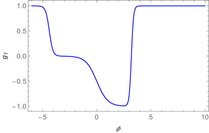
(a)  $g_{1}(\phi)$

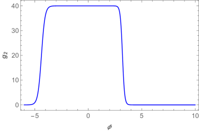
(b)  $g_{2}(\phi)$

Figure 1: The functions $g_{1}(\phi)$ and $g_{2}(\phi)$, where we have set $q_{1}=10$, $q_{2}=6$, $q_{3}=10$, $\phi_{0}=3.2$, $\phi_{3}=-4.38$, $f_{1}=1$, $f_{2}=40$.

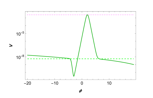
Figure 2: A plot illustrating the potential $V(\phi)$ with parameters set as follows: $\phi_{1}=2$, $\phi_{2}=-4$, $\phi_{4}=20$, $\phi_{5}=29$, $q_{2}=6$, $q_{4}=4$, $\lambda=0.01$, $\sigma=23$, and $m=-4.5\times 10^{-6}$. The height of the potential barrier significantly exceeds that of both sides where slow-roll inflation occurs, i.e., $V_{\mathrm{top}}\gg V_{\mathrm{inf1}}$ and $V_{\mathrm{inf2}}$. As the scalar field rolls along the potential from left to right, the universe sequentially experiences the first stage of slow-roll inflation, NEC violation, and the second stage of slow-roll inflation.

To achieve the aforementioned background evolution via NEC violation, we set these $\phi$-dependent functions $g_{1}$, $g_{2}$ and the potential $V$ in action (1) as

$$g_{1}(\phi) = {1\over 1+e^{q_{2}(\phi-\phi_{3})}}-{f_{1}e^{2\phi}\over 1+f_{1}e^{2\phi}}+{2\over 1+e^{-q_{1}(\phi-\phi_{0})}}\,,$$ (5)

$$g_{2}(\phi) = {f_{2}\over 1+e^{-q_{2}(\phi-\phi_{3})}}{1\over 1+e^{q_{3}(\phi-\phi_{0})}}\,,$$ (6)

$$\begin{split}V(\phi)=&{1\over 2}m^{2}(\phi-\phi_{4})^{2}{1\over 1+e^{q_{2}(\phi-\phi_{2})}}+\lambda\left[1-\frac{(\phi-\phi_{1})^{2}}{\sigma^{2}}\right]^{2}{e^{-q_{4}(\phi-\phi_{1})}\over{(1+e^{-q_{4}(\phi-\phi_{1})})}^{2}}\\ &+{1\over 2}m^{2}(\phi-\phi_{5})^{2}{1\over 1+e^{-q_{4}(\phi-\phi_{1})}}\,,\end{split}$$ (7)

where $\lambda$, $m$, $f_{1,2}$, $q_{1,2,3,4}$ and $\phi_{0,1,2,3,4,5}$ are dimensionless constants. We plot $g_{1}(\phi)$, $g_{2}(\phi)$ and $V(\phi)$ for appropriate values of these parameters in Figs. 1 and 2. As the scalar field rolls along the potential from left to right, the universe sequentially experiences the first stage of slow-roll inflation, NEC violation, and the second stage of slow-roll inflation. These two slow-roll stages are labeled as “inf1” and “inf2” respectively.

The parameters introduced above should satisfy $\phi_{3}<\phi_{2}<0<\phi_{1}<\phi_{0}$. As can be seen in Figs. 1 and 2, when $\phi$ is much smaller than $\phi_{3}$, $g_{1}=1$ and $g_{2}=0$, rendering the potential responsible for the first stage of slow-roll inflation. In this regime, the first term of the potential predominates. Conversely, as $\phi$ greatly exceeds $\phi_{0}$, $g_{1}=1$ and $g_{2}=0$, and the potential is responsible for the second stage of slow-roll inflation, with the third term in the potential becoming dominant. The exponential term in each expression serves to modulate the dominance of various terms across different regions of the potential.

From Fig. 2, it can be observed that the height of the potential barrier significantly exceeds that of both sides where slow-roll inflation occurs. For a slowly rolling canonical scalar field, such a high barrier is insurmountable. However, with the action described in Eq. (1) and via the NEC violation mechanism, the scalar field can naturally disrupt the slow-roll conditions and rapidly climb over the barrier.

We numerically solve the background evolutions and display the evolutions of $\phi$, $\dot{\phi}$, $H$, $(aH)^{-1}$ and $\epsilon\equiv-\dot{H}/H^{2}$ in Figs. 3, 4 and 5. From these figures, we can see that the universe sequentially experiences the first stage of slow-roll inflation, NEC violation, and the second stage of slow-roll inflation. This background evolution is similar to that in the scenario described in Cai:2020qpu . The main difference from the model in Cai:2020qpu lies in the fact that in this model, the energy scales of the first and second stages of slow-roll inflation are closer to each other.

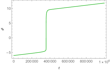
(a)

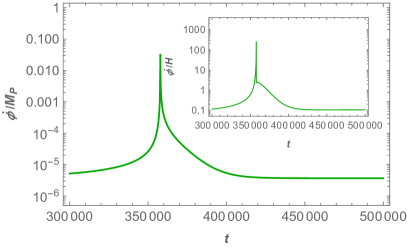
(b)

Figure 3: The evolutions of $\phi(t)$ (left panel) and $\dot{\phi}$ (right panel), where $\phi(t_{\rm ini})=-6$, $\dot{\phi}(t_{\rm ini})=0$, $t_{\rm ini}=0$, $\phi_{0}=3.2$, $\phi_{1}=2$, $\phi_{2}=-4$, $\phi_{3}=-4.38$, $q_{1}=10$, $q_{2}=6$, $q_{3}=10$, $q_{4}=4$, $f_{1}=1$, $f_{2}=40$, $\lambda=0.01$, $\sigma=23$ and $m=-4.5\times 10^{-6}$.

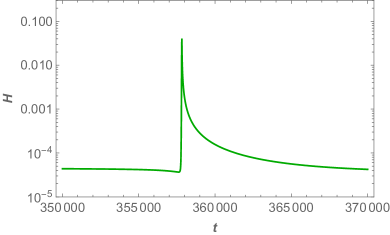
(a)   $H$

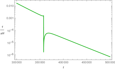
(b)   $(aH)^{-1}$

Figure 4: The evolutions of $H$ (left panel) and the conformal Hubble horizon $(aH)^{-1}$ (right panel).

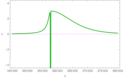
(a)

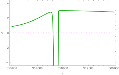
(b)

Figure 5: The evolution of $\epsilon=-\dot{H}/H^{2}$. We have $0<\epsilon\ll 1$ during the first and second stages of slow-roll inflation, and $\epsilon\ll-1$ during the NEC-violating stage.

III The power spectrum of Primordial GWs

In this section, we calculate the power spectrum of primordial GWs for our model. The quadratic actions of tensor perturbation mode $\gamma_{ij}$ can be given as

$$S^{(2)}_{\gamma}={M_{p}^{2}\over 8}\int d^{4}xa^{3}\left[\dot{\gamma}_{ij}^{2}-{(\partial_{k}\gamma_{ij})^{2}\over a^{2}}\right]\,.$$ (8)

In the momentum space,

$$\gamma_{ij}(\tau,\mathbf{x})=\int\frac{d^{3}k}{(2\pi)^{3}}e^{-i\mathbf{k}\cdot\mathbf{x}}\sum_{\lambda=+,\times}\hat{\gamma}_{\lambda}(\tau,\mathbf{k})\epsilon^{(\lambda)}_{ij}(\mathbf{k}),$$ (9)

where $\hat{\gamma}_{\lambda}(\tau,\mathbf{k})=\gamma_{\lambda}(\tau,k)a_{\lambda}(\mathbf{k})+\gamma_{\lambda}^{*}(\tau,-k)a_{\lambda}^{{\dagger}}(-\mathbf{k})$, $\epsilon_{ij}^{(\lambda)}(\mathbf{k})$ satisfies $k_{j}\epsilon_{ij}^{(\lambda)}(\mathbf{k})=0$, $\epsilon_{ii}^{(\lambda)}(\mathbf{k})=0$, $\epsilon_{ij}^{(\lambda)}(\mathbf{k})\epsilon_{ij}^{*(\lambda^{\prime})}(\mathbf{k})=\delta_{\lambda\lambda^{\prime}}$ and $\epsilon_{ij}^{*(\lambda)}(\mathbf{k})=\epsilon_{ij}^{(\lambda)}(-\mathbf{k})$; $a_{\lambda}(\mathbf{k})$ and $a^{{\dagger}}_{\lambda}(\mathbf{k}^{\prime})$ satisfy $[a_{\lambda}(\mathbf{k}),a_{\lambda^{\prime}}^{{\dagger}}(\mathbf{k}^{\prime})]=\delta_{\lambda\lambda^{\prime}}\delta^{(3)}(\mathbf{k}-\mathbf{k}^{\prime})$.

Using the Eq. (8), we can obtain the equation of motion for ${\gamma}_{\lambda}(\tau,\mathbf{k})$ as

$$u_{k}^{\prime\prime}+\left(k^{2}-\frac{a^{\prime\prime}}{a}\right)u_{k}=0\,,$$ (10)

where $u_{k}\equiv\gamma_{\lambda}(\tau,k)aM_{p}/2$ and a prime denotes $d/d\tau$. The power spectrum of primordial GWs is defined as

$$P_{T}={k^{3}\over 2\pi^{2}}\sum_{\lambda=+,\times}|\gamma_{\lambda}|^{2}=\frac{4k^{3}}{\pi^{2}M_{p}^{2}}\cdot\frac{\left|u_{k}\right|^{2}}{a^{2}}\,,$$ (11)

which should be evaluated at the end of the second stage of slow-roll inflation.

We numerically solve Eq. (10) and obtain the power spectrum of primordial GWs for our model. The results are displayed in Fig. 6. We observe a significant enhancement in the power spectrum amplitude of perturbation modes that exit the horizon around the NEC violation epoch in this model. This is because perturbation modes that are outside the horizon during the NEC violation period experience rapid growth, surpassing the amplitude of the constant mode. Therefore, the power spectrum at intermediate scales exhibits a blue tilt. Similar to the model in Ref. Cai:2020qpu , the model in this paper also has the potential to explain observations at the PTA scale. However, unlike the model in Ref. Cai:2020qpu , the power spectrum amplitudes of perturbation modes that exit the horizon during the second stage of slow-roll inflation are not significantly different from those that exit during the first stage.

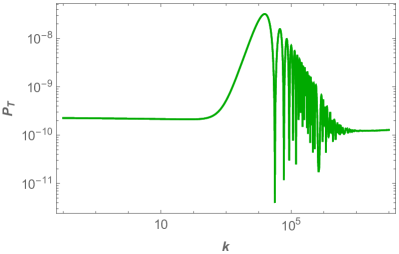
(a)  $P_{T}$

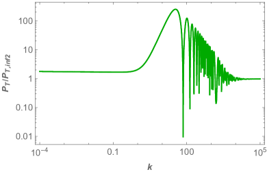
(b)  $P_{T}/P_{T,\text{inf2}}$

Figure 6: The power spectra $P_{T}$ of primordial GWs for our model obtained by numerically solving Eq. (10). We have set $q_{1}=10$, $q_{2}=6$, $q_{3}=10$, $q_{4}=4$, $\phi_{0}=3.2$, $\phi_{1}=2$, $\phi_{2}=-4$, $\phi_{3}=-4.38$, $\phi_{4}=20$, $\phi_{5}=29$, $f_{1}=1$, $f_{2}=40$, $\lambda=0.01$, $\sigma=23$, $m=-4.5\times 10^{-6}$, $\phi(t_{\rm ini})=-6$, $\dot{\phi}(t_{\rm ini})=0$ and $t_{\rm ini}=0$.

In the following, we attempt to provide an analytical derivation of the power spectrum. Analogous to the approach in Ref. Cai:2020qpu , we divide the background evolution in this model into four stages, with the scale factor of the $j$-th stage approximately parameterized as

$$a_{j}(\tau)\sim\left({\tau}_{R,j}-\tau\right)^{\frac{1}{\epsilon_{j}-1}},$$ (12)

where $\epsilon_{j}\equiv-\dot{H_{j}}/H_{j}^{2}={3\over 2}(1+w_{j})$, ${\tau}_{R,j}\equiv\tau_{j}-(\epsilon_{j}-1)^{-1}\mathcal{H}^{-1}(\tau_{j})$, $j=1$, 2, 3, 4. For simplicity, we assume $\epsilon_{j}$ (i.e., the equation of state parameter $w_{j}$) as a constant. We also require continuity of $a$ and $a^{\prime}$ at each transition moment.

With Eq. (12), we have

$$\frac{a_{j}^{\prime\prime}}{a_{j}}={\nu_{j}^{2}-{1/4}\over{(\tau-\tau_{R,j})^{2}}}\,,$$ (13)

where $\nu_{j}={3\over 2}\left|{1-w_{j}\over 1+3w_{j}}\right|$. Consequently, the solutions to Eq. (10) for each phase can be given as

$$u_{k,1}(\tau) = {\sqrt{\pi(\tau_{R,1}-\tau)}\over 2}\left\{\alpha_{1}H_{\nu_{1}}^{(1)}[k(\tau_{R,1}-\tau)]+\beta_{1}H_{\nu_{1}}^{(2)}[k(\tau_{R,1}-\tau)]\right\},\,\,(\tau<\tau_{1})\,,$$ (14)

$$u_{k,{2}}(\tau) = {\sqrt{\pi(\tau_{R,{2}}-\tau)}\over 2}\Big{\{}\alpha_{2}H_{\nu_{2}}^{(1)}[k(\tau_{R,2}-\tau)]+\beta_{2}H_{\nu_{2}}^{(2)}[k(\tau_{R,2}-\tau)]\Big{\}},(\tau_{1}\leq\tau\leq\tau_{2})\,,$$

$$u_{k,{3}}(\tau) = {\sqrt{\pi(\tau_{R,{3}}-\tau)}\over 2}\Big{\{}\alpha_{3}H_{\nu_{3}}^{(1)}[k(\tau_{R,3}-\tau)]+\beta_{3}H_{\nu_{3}}^{(2)}[k(\tau_{R,3}-\tau)]\Big{\}},(\tau_{2}<\tau\leq\tau_{3})\,,$$

$$u_{k,{4}}(\tau) = {\sqrt{\pi(\tau_{R,{4}}-\tau)}\over 2}\Big{\{}\alpha_{4}H_{\nu_{4}}^{(1)}[k(\tau_{R,4}-\tau)]+\beta_{4}H_{\nu_{4}}^{(2)}[k(\tau_{R,4}-\tau)]\Big{\}},(\tau_{3}<\tau\leq\tau_{4})\,,$$

where $\alpha_{j}$ and $\beta_{j}$ are $k$-dependent coefficients, $j=1$, 2, 3, 4. We set the initial state as the Bunch-Davis vacuum, i.e., $u_{k}=e^{-ik\tau}/\sqrt{2k}$, which indicates that $|\alpha_{1}|=1$ and $|\beta_{1}|=0$.

Using the matching conditions $u_{k,j}(\tau_{j})=u_{k,j+1}(\tau_{j})$ and $u_{k,j}^{\prime}\big{|}{\tau=\tau{j}}=u_{k,j+1}^{\prime}\big{|}{\tau=\tau{j}}$, we can obtain all of the $\alpha_{j}$ and $\beta_{j}$ for $j=2$, 3, 4. We have

$$\left(\begin{array}[]{ccc}\alpha_{j+1}\\ \beta_{j+1}\end{array}\right) = {\cal M}^{(j)}\left(\begin{array}[]{ccc}\alpha_{j}\\ \beta_{j}\end{array}\right)\,,\quad{\rm where}\quad{\cal M}^{(j)}=\left(\begin{array}[]{ccc}{\cal M}^{(j)}_{11}&{\cal M}^{(j)}_{12}\\ {\cal M}^{(j)}_{21}&{\cal M}^{(j)}_{22}\end{array}\right)\,,$$ (21)

The details of the matrix elements of the transfer matrix can be found in Cai:2015nya ; Cai:2019hge . At the end of the second slow-roll inflation, the power spectrum can be given as

$$P_{T}=\frac{4k^{3}}{\pi^{2}M_{p}^{2}}\cdot\frac{\left|u_{k,4}\right|^{2}}{a^{2}}\Big{|}_{\tau\rightarrow\tau_{4}}=P_{T,inf2}\left|\alpha_{4}-\beta_{4}\right|^{2}\,,$$ (22)

where $P_{T,inf2}={2H_{inf2}^{2}\over\pi^{2}M_{p}^{2}}$. A detailed expression for $\alpha_{4}$ and $\beta_{4}$ can be found in Appendix A. We plot $P_{T}/P_{T,\text{inf2}}=\left|\alpha_{4}-\beta_{4}\right|^{2}$ in Fig. 7 for different choices of $w_{i}$. We can see from Figs. 6(b) and 7(a) that the approximation works well for our model with appropriate choices of $w_{i}$. In our parameterization, the height difference between the two platforms in the potential can be adjusted by changing $\epsilon_{3}=-\dot{H}/H^{2}={3\over 2}(1+w_{j})$.

(a)

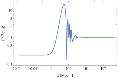
(b)

Figure 7: The power spectrum of the primordial GWs given by Eq. (22). For the left panel, we set $w_{1}=-1$, $w_{2}=-10$, $w_{3}=1$, and $w_{4}=-1$, providing a close approximation to the result shown in Fig. 6(b). In the right panel, we choose $w_{1}=-1$, $w_{2}=-10$, $w_{3}=2/3$, and $w_{4}=-1$, resembling the scenario discussed in Ref. Cai:2020qpu .

IV The energy density spectrum of GWs

The energy density spectrum of GWs Turner:1993vb ; Boyle:2005se (see also Zhao:2006mm ; Kuroyanagi:2014nba ) is

$$\Omega_{GW}(\tau_{0})=\frac{k^{2}}{12a_{0}^{2}H^{2}_{0}}P_{T}(k)\left[\frac{3\Omega_{{m}}j_{1}(k\tau_{0})}{k\tau_{0}}\sqrt{1.0+1.36\frac{k}{k_{\text{eq}}}+2.50\left(\frac{k}{k_{\text{eq}}}\right)^{2}}\right]^{2},$$ (23)

where $H_{0}=67.8\,{\rm km/s/Mpc}$, $\tau_{0}=1.41\times 10^{4}$ Mpc, $a_{0}=1$, $k_{\text{eq}}=0.073\,\Omega_{\text{m}}h^{2}$ Mpc^-1 is the wavenumber corresponding to the mode that entered the horizon at the equality of matter and radiation, $\Omega_{\rm m}=\rho_{m}/\rho_{c}$ is the density fraction of matter today, $\rho_{{c}}=3H^{2}_{0}/\big{(}8\pi G\big{)}$ is the critical energy density, and $j_{1}(x)$ is the spherical Bessel function of the first kind. We plot the energy density spectrum of GWs for our model in Figs. 8(a) and 8(b), using both the numerical results obtained by solving Eq. (10) and the analytical results provided by Eq. (22), respectively. Namely, Figs. 8(a) and 8(b) correspond to the power spectra displayed in Figs. 6(a) and 7(a), respectively.

(a)

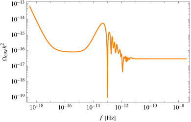
(b)

Figure 8: The energy density spectrum of GWs for our model obtained by using both the numerical results obtained by solving Eq. (10) (left panel) and the analytical results provided by Eq. (22) (right panel).

Comparing Figs. 8(a) and 8(b), we observe a good agreement between the energy density spectra obtained by the two methods. In the second case, where the slow-roll parameters are approximated as constants, some details of the mode evolution are not fully reflected. For observational purposes, the distinctive features may include the blue-tilted nature in the middle-frequency range and the decreasing amplitude of these oscillations at higher frequencies.

V Conclusion

In this paper, we propose a new single-field model where the universe sequentially undergoes a first stage of slow-roll inflation, NEC violation, and a second stage of slow-roll inflation. Within the potential responsible for slow-roll inflation, there exists a high barrier, over which the rolling inflaton climb via the NEC violation mechanism before entering the second inflationary stage. Following the NEC violation, there is a process of energy scale reduction, resulting in the energy scales of the two slow-roll inflation stages being relatively close, contrasting with the model in Cai:2020qpu .

We calculate the power spectrum of primordial GWs using both numerical and analytical methods, comparing the results obtained from these two approaches. We find that the approximation used in the analytical derivation closely matches the results from numerical calculations. The power spectrum is nearly scale-invariant on both large and small scales. However, in the middle-frequency range, it shows a blue-tilted nature, while at higher frequencies, there is a reduction in oscillation amplitudes. These unique characteristics could potentially differentiate our model from others.

In the early universe, NEC violation may have occurred multiple times. We present a sketch of the GW power spectrum in Fig. 9 for the scenario where $\phi$ climbs over the potential barriers multiple times. The accumulation of future observational data from various frequency bands, including CMB, PTA, Advanced LIGO, Advanced Virgo, LISA, Taiji and Tianqin, will enable more tests or constraints on NEC violation in the very early universe.

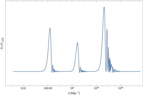
Figure 9: A sketch of the GW power spectrum for the scenario where $\phi$ climbs over the potential barriers multiple times.

Appendix A Detailed analytic expression of $\alpha$ and $\beta$

The scale factor can be parameterized as a piecewise function of $\tau$, i.e.,

$$a_{j}(\tau)=a_{j}(\tau_{j})\left(\frac{\tau-\tau_{R,j}}{\tau_{j}-\tau_{R,j}}\right)^{\frac{1}{\epsilon_{j}-1}}~{},\quad\tau<\tau_{j}\,.$$ (24)

The continuity of $a$ gives

$$a_{1}(\tau_{1})=a_{2}(\tau_{2})\left(\frac{\tau_{1}-\tau_{R,2}}{\tau_{2}-\tau_{R,2}}\right)^{\frac{1}{\epsilon_{2}-1}},$$ (25)

$$a_{2}(\tau_{2})=a_{3}(\tau_{3})\left(\frac{\tau_{2}-\tau_{R,3}}{\tau_{3}-\tau_{R,3}}\right)^{\frac{1}{\epsilon_{3}-1}},~{}$$ (26)

$$a_{3}(\tau_{3})=a_{4}(\tau_{4})\left(\frac{\tau_{3}-\tau_{R,4}}{\tau_{4}-\tau_{R,4}}\right)^{\frac{1}{\epsilon_{4}-1}}.$$ (27)

Considering the continuity of $a^{\prime}$ or $\mathcal{H}$, we can define the following quantities:

$$\bar{\mathcal{H}}_{1}\equiv\mathcal{H}(\tau_{1})~{},~{}\bar{\mathcal{H}}_{2}\equiv\mathcal{H}(\tau_{2})~{},~{}\bar{\mathcal{H}}_{3}\equiv\mathcal{H}(\tau_{3})~{}.$$ (28)

Using (24), we can obtain the integration constants $\tau_{R,j}$ as

$$\tau_{R,1}=\tau_{1}+\bar{\mathcal{H}}_{1}^{-1}~{},~{}\tau_{R,2}=\tau_{1}+({v_{2}-\frac{1}{2}}){\bar{\mathcal{H}}_{1}^{-1}},\tau_{R,2}=\tau_{2}+({v_{2}-\frac{1}{2}}){\bar{\mathcal{H}}_{2}^{-1}},$$ (29)

$$\tau_{R,3}=\tau_{2}+({-v_{3}-\frac{1}{2}}){\bar{\mathcal{H}}_{2}^{-1}},\tau_{R,3}=\tau_{3}+({-v_{3}-\frac{1}{2}}){\bar{\mathcal{H}}_{3}^{-1}},~{}\tau_{R,4}=\tau_{3}+\bar{\mathcal{H}}_{3}^{-1},$$ (30)

where $\nu_{j}={3\over 2}\left|{1-w_{j}\over 1+3w_{j}}\right|$, and $\epsilon_{j}={3\over 2}(1+w_{j})\simeq{\rm const.}$. Note that for $-{1\over 3}<w_{j}<1$ and $w_{j}<-{1\over 3}$, we have $\nu_{j}=-{1\over 2}-{1\over 1-\epsilon_{j}}$ and $\nu_{j}={1\over 2}+{1\over 1-\epsilon_{j}}$, respectively.

Using the matching method, we obtain the following recursive relations:

$$~{}~{}~{}~{}~{}~{}\alpha_{2} =\frac{i\pi}{8x_{1}}\sqrt{\frac{x_{1}}{x_{2}}}\left(H_{\frac{3}{2}}^{(1)}(x_{1})\left(2x_{1}x_{2}H_{\nu_{2}-1}^{(2)}(x_{2})+\left(-2\nu_{2}x_{1}+x_{1}+2x_{2}\right)H_{\nu_{2}}^{(2)}(x_{2})\right)\right.$$

$$\quad-2x_{1}x_{2}H_{\frac{1}{2}}^{(1)}(x_{1})H_{\nu_{2}}^{(2)}(x_{2})\Big{)},$$ (31)

$$~{}~{}~{}~{}~{}~{}~{}~{}~{}\beta_{2} =-\frac{i\pi}{8x_{1}}\sqrt{\frac{x_{1}}{x_{2}}}\left(H_{\frac{3}{2}}^{(1)}(x_{1})\left(2x_{1}x_{2}H_{\nu_{2}-1}^{(1)}(x_{2})+\left(-2\nu_{2}x_{1}+x_{1}+2x_{2}\right)H_{\nu_{2}}^{(1)}(x_{2})\right)\right.$$

$$\quad-2x_{1}x_{2}H_{\frac{1}{2}}^{(1)}(x_{1})H_{\nu_{2}}^{(1)}(x_{2})\Big{)},$$ (32)

$$\alpha_{3} =-\frac{\pi}{8y_{1}}\sqrt{-\frac{y_{1}}{y_{2}}}\Big{(}y_{2}H_{\nu_{3}}^{(2)}(y_{2})\Big{(}2\alpha_{2}y_{1}H_{\nu_{2}-1}^{(1)}(y_{1})+(\alpha_{2}-2\alpha_{2}\nu_{2})H_{\nu_{2}}^{(1)}(y_{1})$$

$$\quad+2\beta_{2}y_{1}H_{\nu_{2}-1}^{(2)}(y_{1})+(\beta_{2}-2\beta_{2}\nu_{2})H_{\nu_{2}}^{(2)}(y_{1})\Big{)}$$

$$\quad-y_{1}\Big{(}2y_{2}H_{\nu_{3}-1}^{(2)}(y_{2})+(1-2\nu_{3})H_{\nu_{3}}^{(2)}(y_{2})\Big{)}$$

$$\quad\cdot\Big{(}\alpha_{2}H_{\nu_{2}}^{(1)}(y_{1})+\beta_{2}H_{\nu_{2}}^{(2)}(y_{1})\Big{)}\Big{)},$$ (33)

$$\beta_{3} =\frac{\pi}{8y_{1}}\sqrt{-\frac{y_{1}}{y_{2}}}\Big{(}2\alpha_{2}y_{1}y_{2}H_{\nu_{2}-1}^{(1)}(y_{1})H_{\nu_{3}}^{(1)}(y_{2})$$

$$\quad+\alpha_{2}H_{\nu_{2}}^{(1)}(y_{1})\Big{(}\big{(}2\nu_{3}y_{1}-2\nu_{2}y_{2}-y_{1}+y_{2}\big{)}H_{\nu_{3}}^{(1)}(y_{2})-2y_{1}y_{2}H_{\nu_{3}-1}^{(1)}(y_{2})\Big{)}$$

$$\quad-2\beta_{2}y_{1}y_{2}H_{\nu_{3}-1}^{(1)}(y_{2})H_{\nu_{2}}^{(2)}(y_{1})+\beta_{2}H_{\nu_{3}}^{(1)}(y_{2})\Big{(}2y_{1}y_{2}H_{\nu_{2}-1}^{(2)}(y_{1})$$

$$\quad+\big{(}2\nu_{3}y_{1}-2\nu_{2}y_{2}-y_{1}+y_{2}\big{)}H_{\nu_{2}}^{(2)}(y_{1})\Big{)}\Big{)},$$ (34)

$$\alpha_{4} =\frac{\pi}{8z_{1}}\sqrt{-\frac{z_{1}}{z_{2}}}\Big{(}2z_{1}\Big{(}H_{\frac{3}{2}}^{(2)}(z_{2})-z_{2}H_{\frac{1}{2}}^{(2)}(z_{2})\Big{)}\Big{(}\alpha_{3}H_{\nu_{3}}^{(1)}(z_{1})+\beta_{3}H_{\nu_{3}}^{(2)}(z_{1})\Big{)}$$

$$\quad+z_{2}H_{\frac{3}{2}}^{(2)}(z_{2})\Big{(}2\alpha_{3}z_{1}H_{\nu_{3}-1}^{(1)}(z_{1})+\big{(}\alpha_{3}-2\alpha_{3}\nu_{3}\big{)}H_{\nu_{3}}^{(1)}(z_{1})$$

$$\quad+2\beta_{3}z_{1}H_{\nu_{3}-1}^{(2)}(z_{1})+\big{(}\beta_{3}-2\beta_{3}\nu_{3}\big{)}H_{\nu_{3}}^{(2)}(z_{1})\Big{)}\Big{)},$$ (35)

$$\begin{split}\beta_{4}&=-\frac{\pi}{8z_{1}}\sqrt{-\frac{z_{1}}{z_{2}}}\Big{(}H_{\frac{3}{2}}^{(1)}(z_{2})\Big{(}2\alpha_{3}z_{1}z_{2}H_{\nu_{3}-1}^{(1)}(z_{1})\\ &\quad+\alpha_{3}\big{(}-2\nu_{3}z_{2}+2z_{1}+z_{2}\big{)}H_{\nu_{3}}^{(1)}(z_{1})\\ &\quad+2\beta_{3}z_{1}z_{2}H_{\nu_{3}-1}^{(2)}(z_{1})+\beta_{3}\big{(}-2\nu_{3}z_{2}+2z_{1}+z_{2}\big{)}H_{\nu_{3}}^{(2)}(z_{1})\Big{)}\\ &\quad-2z_{1}z_{2}H_{\frac{1}{2}}^{(1)}(z_{2})\Big{(}\alpha_{3}H_{\nu_{3}}^{(1)}(z_{1})+\beta_{3}H_{\nu_{3}}^{(2)}(z_{1})\Big{)}\Big{)},\end{split}$$ (36)

where $x_{1}=k(\tau_{R,1}-\tau_{1})$, $x_{2}=k(\tau_{R,2}-\tau_{1})$, $y_{1}=k(\tau_{R,2}-\tau_{2})$, $y_{2}=k(\tau_{R,3}-\tau_{2})$, $z_{1}=k(\tau_{R,3}-\tau_{3})$, $z_{2}=k(\tau_{R,4}-\tau_{3})$. Since the results are too complex, we only provide the recursive formulas for $\alpha_{j}$ and $\beta_{j}$.

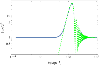
(a)

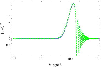
(b)

Figure 10: Left: Comparison between $|G_{1}|^{2}$ (green dashed curve) and the numerical result of ${P_{T}/P_{T,inf2}}$ (blue dotted curve). Right: Comparison between the template (38) (green dashed curve) and the numerical result of ${P_{T}/P_{T,inf2}}$ (blue dotted curve). We have set $\bar{\cal H}_{1}=10^{4}a_{0}H_{0}$, where $a_{0}=1$ and $H_{0}=67\,{\rm km/s/Mpc}$. We also set $w_{2}=-15$ and $w_{3}={2}/{3}$, which corresponding to $\nu_{2}={6}/{11}$ and $\nu_{3}={1}/{6}$, respectively.

Next, we attempt to explore potential approximations. It’s worth noting that in our model, $y_{2}$ and $z_{1}$ are negative. Therefore, our approach here is to consider $k\gg\bar{\mathcal{H}}_{1}$. By series expansion, we get

$$G_{1} ={\alpha_{4}-\beta_{4}}$$ (37)

$$=\frac{\pi^{3/2}}{16\sqrt{2}z_{2}^{2}}\bigg{(}2H_{\nu_{2}-1}^{(1)}\left(y_{1}\right)\bigg{(}H_{\nu_{3}}^{(1)}\left(y_{2}\right)\bigg{(}2H_{\nu_{3}-1}^{(2)}\left(z_{1}\right)\sqrt{y_{1}y_{2}z_{1}}z_{2}\left(\cos\left(z_{2}\right)z_{2}-\sin\left(z_{2}\right)\right)$$

$$+H_{\nu_{3}}^{(2)}\left(z_{1}\right)\bigg{(}\sin\left(z_{2}\right)\left(2\sqrt{y_{1}y_{2}z_{1}}z_{2}^{2}+\sqrt{\frac{y_{1}y_{2}}{z_{1}}}\left(1-2\nu_{3}\right)z_{2}-2\sqrt{y_{1}y_{2}z_{1}}\right)$$

$$+\cos\left(z_{2}\right)z_{2}\left(\sqrt{\frac{y_{1}y_{2}}{z_{1}}}z_{2}\left(2\nu_{3}-1\right)+2\sqrt{y_{1}y_{2}z_{1}}\right)\bigg{)}\bigg{)}$$

$$+H_{\nu_{3}}^{(2)}\left(y_{2}\right)\bigg{(}H_{\nu_{3}}^{(1)}\left(z_{1}\right)\bigg{(}\sin\left(z_{2}\right)\left(-2\sqrt{y_{1}y_{2}z_{1}}z_{2}^{2}+\sqrt{\frac{y_{1}y_{2}}{z_{1}}}\left(2\nu_{3}-1\right)z_{2}+2\sqrt{y_{1}y_{2}z_{1}}\right)$$

$$-\cos\left(z_{2}\right)z_{2}\left(\sqrt{\frac{y_{1}y_{2}}{z_{1}}}z_{2}\left(2\nu_{3}-1\right)+2\sqrt{y_{1}y_{2}z_{1}}\right)\bigg{)}-2H_{\nu_{3}-1}^{(1)}\left(z_{1}\right)\sqrt{y_{1}y_{2}z_{1}}z_{2}\big{(}\cos\left(z_{2}\right)z_{2}$$

$$-\sin\left(z_{2}\right)\big{)}\bigg{)}\bigg{)}+H_{\nu_{2}}^{(1)}\left(y_{1}\right)\bigg{(}-4\cos\left(z_{2}\right)H_{\nu_{3}}^{(1)}\left(y_{2}\right)H_{\nu_{3}}^{(2)}\left(z_{1}\right)\sqrt{\frac{y_{1}}{y_{2}z_{1}}}\nu_{3}^{2}z_{2}^{2}$$

$$+2\cos\left(z_{2}\right)H_{\nu_{3}}^{(1)}\left(y_{2}\right)H_{\nu_{3}}^{(2)}\left(z_{1}\right)\sqrt{\frac{y_{2}}{y_{1}z_{1}}}\nu_{2}z_{2}^{2}-4\cos\left(z_{2}\right)H_{\nu_{3}}^{(1)}\left(y_{2}\right)H_{\nu_{3}-1}^{(2)}\left(z_{1}\right)\sqrt{\frac{y_{2}z_{1}}{y_{1}}}\nu_{2}z_{2}^{2}$$

$$-4H_{\nu_{3}}^{(1)}\left(y_{2}\right)H_{\nu_{3}}^{(2)}\left(z_{1}\right)\sin\left(z_{2}\right)\sqrt{\frac{y_{2}z_{1}}{y_{1}}}\nu_{2}z_{2}^{2}-4\cos\left(z_{2}\right)H_{\nu_{3}}^{(1)}\left(y_{2}\right)H_{\nu_{3}}^{(2)}\left(z_{1}\right)\sqrt{\frac{y_{2}}{y_{1}z_{1}}}\nu_{2}\nu_{3}z_{2}^{2}$$

$$+4\cos\left(z_{2}\right)H_{\nu_{3}}^{(1)}\left(y_{2}\right)H_{\nu_{3}}^{(2)}\left(z_{1}\right)\sqrt{\frac{y_{1}}{y_{2}z_{1}}}\nu_{3}z_{2}^{2}+2\cos\left(z_{2}\right)H_{\nu_{3}}^{(1)}\left(y_{2}\right)H_{\nu_{3}}^{(2)}\left(z_{1}\right)\sqrt{\frac{y_{2}}{y_{1}z_{1}}}\nu_{3}z_{2}^{2}$$

$$-4\cos\left(z_{2}\right)H_{\nu_{3}-1}^{(1)}\left(y_{2}\right)H_{\nu_{3}}^{(2)}\left(z_{1}\right)\sqrt{\frac{y_{1}y_{2}}{z_{1}}}\nu_{3}z_{2}^{2}-4\cos\left(z_{2}\right)H_{\nu_{3}}^{(1)}\left(y_{2}\right)H_{\nu_{3}-1}^{(2)}\left(z_{1}\right)\sqrt{\frac{y_{1}z_{1}}{y_{2}}}\nu_{3}z_{2}^{2}$$

$$-4H_{\nu_{3}}^{(1)}\left(y_{2}\right)H_{\nu_{3}}^{(2)}\left(z_{1}\right)\sin\left(z_{2}\right)\sqrt{\frac{y_{1}z_{1}}{y_{2}}}\nu_{3}z_{2}^{2}-\cos\left(z_{2}\right)H_{\nu_{3}}^{(1)}\left(y_{2}\right)H_{\nu_{3}}^{(2)}\left(z_{1}\right)\sqrt{\frac{y_{1}}{y_{2}z_{1}}}z_{2}^{2}$$

$$-\cos\left(z_{2}\right)H_{\nu_{3}}^{(1)}\left(y_{2}\right)H_{\nu_{3}}^{(2)}\left(z_{1}\right)\sqrt{\frac{y_{2}}{y_{1}z_{1}}}z_{2}^{2}+2\cos\left(z_{2}\right)H_{\nu_{3}-1}^{(1)}\left(y_{2}\right)H_{\nu_{3}}^{(2)}\left(z_{1}\right)\sqrt{\frac{y_{1}y_{2}}{z_{1}}}z_{2}^{2}$$

$$+2\cos\left(z_{2}\right)H_{\nu_{3}}^{(1)}\left(y_{2}\right)H_{\nu_{3}-1}^{(2)}\left(z_{1}\right)\sqrt{\frac{y_{1}z_{1}}{y_{2}}}z_{2}^{2}+2H_{\nu_{3}}^{(1)}\left(y_{2}\right)H_{\nu_{3}}^{(2)}\left(z_{1}\right)\sin\left(z_{2}\right)\sqrt{\frac{y_{1}z_{1}}{y_{2}}}z_{2}^{2}$$

$$+2\cos\left(z_{2}\right)H_{\nu_{3}}^{(1)}\left(y_{2}\right)H_{\nu_{3}-1}^{(2)}\left(z_{1}\right)\sqrt{\frac{y_{2}z_{1}}{y_{1}}}z_{2}^{2}+2H_{\nu_{3}}^{(1)}\left(y_{2}\right)H_{\nu_{3}}^{(2)}\left(z_{1}\right)\sin\left(z_{2}\right)\sqrt{\frac{y_{2}z_{1}}{y_{1}}}z_{2}^{2}$$

$$-4\cos\left(z_{2}\right)H_{\nu_{3}-1}^{(1)}\left(y_{2}\right)H_{\nu_{3}-1}^{(2)}\left(z_{1}\right)\sqrt{y_{1}y_{2}z_{1}}z_{2}^{2}-4H_{\nu_{3}-1}^{(1)}\left(y_{2}\right)H_{\nu_{3}}^{(2)}\left(z_{1}\right)\sin\left(z_{2}\right)\sqrt{y_{1}y_{2}z_{1}}z_{2}^{2}$$

$$+4H_{\nu_{3}}^{(1)}\left(y_{2}\right)H_{\nu_{3}}^{(2)}\left(z_{1}\right)\sin\left(z_{2}\right)\sqrt{\frac{y_{1}}{y_{2}z_{1}}}\nu_{3}^{2}z_{2}-2H_{\nu_{3}}^{(1)}\left(y_{2}\right)H_{\nu_{3}}^{(2)}\left(z_{1}\right)\sin\left(z_{2}\right)\sqrt{\frac{y_{2}}{y_{1}z_{1}}}\nu_{2}z_{2}$$

$$-4\cos\left(z_{2}\right)H_{\nu_{3}}^{(1)}\left(y_{2}\right)H_{\nu_{3}}^{(2)}\left(z_{1}\right)\sqrt{\frac{y_{2}z_{1}}{y_{1}}}\nu_{2}z_{2}+4H_{\nu_{3}}^{(1)}\left(y_{2}\right)H_{\nu_{3}-1}^{(2)}\left(z_{1}\right)\sin\left(z_{2}\right)\sqrt{\frac{y_{2}z_{1}}{y_{1}}}\nu_{2}z_{2}$$

$$+4H_{\nu_{3}}^{(1)}\left(y_{2}\right)H_{\nu_{3}}^{(2)}\left(z_{1}\right)\sin\left(z_{2}\right)\sqrt{\frac{y_{2}}{y_{1}z_{1}}}\nu_{2}\nu_{3}z_{2}-4H_{\nu_{3}}^{(1)}\left(y_{2}\right)H_{\nu_{3}}^{(2)}\left(z_{1}\right)\sin\left(z_{2}\right)\sqrt{\frac{y_{1}}{y_{2}z_{1}}}\nu_{3}z_{2}$$

$$-2H_{\nu_{3}}^{(1)}\left(y_{2}\right)H_{\nu_{3}}^{(2)}\left(z_{1}\right)\sin\left(z_{2}\right)\sqrt{\frac{y_{2}}{y_{1}z_{1}}}\nu_{3}z_{2}+4H_{\nu_{3}-1}^{(1)}\left(y_{2}\right)H_{\nu_{3}}^{(2)}\left(z_{1}\right)\sin\left(z_{2}\right)\sqrt{\frac{y_{1}y_{2}}{z_{1}}}\nu_{3}z_{2}$$

$$\begin{split}&-4\cos\left(z_{2}\right)H_{\nu_{3}}^{(1)}\left(y_{2}\right)H_{\nu_{3}}^{(2)}\left(z_{1}\right)\sqrt{\frac{y_{1}z_{1}}{y_{2}}}\nu_{3}z_{2}+4H_{\nu_{3}}^{(1)}\left(y_{2}\right)H_{\nu_{3}-1}^{(2)}\left(z_{1}\right)\sin\left(z_{2}\right)\sqrt{\frac{y_{1}z_{1}}{y_{2}}}\nu_{3}z_{2}\\ &+2H_{\nu_{3}-1}^{(1)}\left(z_{1}\right)\left(\cos\left(z_{2}\right)z_{2}-\sin\left(z_{2}\right)\right)\bigg{(}2\sqrt{y_{1}y_{2}z_{1}}H_{\nu_{3}-1}^{(2)}\left(y_{2}\right)+H_{\nu_{3}}^{(2)}\left(y_{2}\right)\bigg{(}2\sqrt{\frac{y_{2}z_{1}}{y_{1}}}\nu_{2}\\ &+2\sqrt{\frac{y_{1}z_{1}}{y_{2}}}\nu_{3}-\sqrt{\frac{y_{1}z_{1}}{y_{2}}}-\sqrt{\frac{y_{2}z_{1}}{y_{1}}}\bigg{)}\bigg{)}z_{2}+H_{\nu_{3}}^{(1)}\left(y_{2}\right)H_{\nu_{3}}^{(2)}\left(z_{1}\right)\sin\left(z_{2}\right)\sqrt{\frac{y_{1}}{y_{2}z_{1}}}z_{2}\\ &+H_{\nu_{3}}^{(1)}\left(y_{2}\right)H_{\nu_{3}}^{(2)}\left(z_{1}\right)\sin\left(z_{2}\right)\sqrt{\frac{y_{2}}{y_{1}z_{1}}}z_{2}-2H_{\nu_{3}-1}^{(1)}\left(y_{2}\right)H_{\nu_{3}}^{(2)}\left(z_{1}\right)\sin\left(z_{2}\right)\sqrt{\frac{y_{1}y_{2}}{z_{1}}}z_{2}\\ &+2\cos\left(z_{2}\right)H_{\nu_{3}}^{(1)}\left(y_{2}\right)H_{\nu_{3}}^{(2)}\left(z_{1}\right)\sqrt{\frac{y_{1}z_{1}}{y_{2}}}z_{2}-2H_{\nu_{3}}^{(1)}\left(y_{2}\right)H_{\nu_{3}-1}^{(2)}\left(z_{1}\right)\sin\left(z_{2}\right)\sqrt{\frac{y_{1}z_{1}}{y_{2}}}z_{2}\\ &+2\cos\left(z_{2}\right)H_{\nu_{3}}^{(1)}\left(y_{2}\right)H_{\nu_{3}}^{(2)}\left(z_{1}\right)\sqrt{\frac{y_{2}z_{1}}{y_{1}}}z_{2}-2H_{\nu_{3}}^{(1)}\left(y_{2}\right)H_{\nu_{3}-1}^{(2)}\left(z_{1}\right)\sin\left(z_{2}\right)\sqrt{\frac{y_{2}z_{1}}{y_{1}}}z_{2}\\ &-4\cos\left(z_{2}\right)H_{\nu_{3}-1}^{(1)}\left(y_{2}\right)H_{\nu_{3}}^{(2)}\left(z_{1}\right)\sqrt{y_{1}y_{2}z_{1}}z_{2}+4H_{\nu_{3}-1}^{(1)}\left(y_{2}\right)H_{\nu_{3}-1}^{(2)}\left(z_{1}\right)\sin\left(z_{2}\right)\sqrt{y_{1}y_{2}z_{1}}z_{2}\\ &+4H_{\nu_{3}}^{(1)}\left(y_{2}\right)H_{\nu_{3}}^{(2)}\left(z_{1}\right)\sin\left(z_{2}\right)\sqrt{\frac{y_{2}z_{1}}{y_{1}}}\nu_{2}+4H_{\nu_{3}}^{(1)}\left(y_{2}\right)H_{\nu_{3}}^{(2)}\left(z_{1}\right)\sin\left(z_{2}\right)\sqrt{\frac{y_{1}z_{1}}{y_{2}}}\nu_{3}\\ &+H_{\nu_{3}}^{(1)}\left(z_{1}\right)\bigg{(}2H_{\nu_{3}-1}^{(2)}\left(y_{2}\right)\bigg{(}\sin\left(z_{2}\right)\bigg{(}2\sqrt{y_{1}y_{2}z_{1}}z_{2}^{2}+\sqrt{\frac{y_{1}y_{2}}{z_{1}}}\left(1-2\nu_{3}\right)z_{2}-2\sqrt{y_{1}y_{2}z_{1}}\bigg{)}\\ &+\cos\left(z_{2}\right)z_{2}\left(\sqrt{\frac{y_{1}y_{2}}{z_{1}}}z_{2}\left(2\nu_{3}-1\right)+2\sqrt{y_{1}y_{2}z_{1}}\right)\bigg{)}+H_{\nu_{3}}^{(2)}\left(y_{2}\right)\bigg{(}\cos\left(z_{2}\right)z_{2}\bigg{(}4\sqrt{\frac{y_{2}z_{1}}{y_{1}}}\nu_{2}\\ &+4\sqrt{\frac{y_{1}z_{1}}{y_{2}}}\nu_{3}+z_{2}\left(2\nu_{3}-1\right)\left(2\sqrt{\frac{y_{2}}{y_{1}z_{1}}}\nu_{2}+2\sqrt{\frac{y_{1}}{y_{2}z_{1}}}\nu_{3}-\sqrt{\frac{y_{1}}{y_{2}z_{1}}}-\sqrt{\frac{y_{2}}{y_{1}z_{1}}}\right)-2\sqrt{\frac{y_{1}z_{1}}{y_{2}}}\\ &-2\sqrt{\frac{y_{2}z_{1}}{y_{1}}}\bigg{)}+\sin\left(z_{2}\right)\bigg{(}\bigg{(}-2\bigg{(}\sqrt{\frac{y_{1}z_{1}}{y_{2}}}+\sqrt{\frac{y_{2}z_{1}}{y_{1}}}\bigg{)}+4\sqrt{\frac{y_{2}z_{1}}{y_{1}}}\nu_{2}+4\sqrt{\frac{y_{1}z_{1}}{y_{2}}}\nu_{3}\bigg{)}z_{2}^{2}\\ &-\left(2\nu_{3}-1\right)\left(2\sqrt{\frac{y_{2}}{y_{1}z_{1}}}\nu_{2}+2\sqrt{\frac{y_{1}}{y_{2}z_{1}}}\nu_{3}-\sqrt{\frac{y_{1}}{y_{2}z_{1}}}-\sqrt{\frac{y_{2}}{y_{1}z_{1}}}\right)z_{2}+2\bigg{(}-2\sqrt{\frac{y_{2}z_{1}}{y_{1}}}\nu_{2}\\ &-2\sqrt{\frac{y_{1}z_{1}}{y_{2}}}\nu_{3}+\sqrt{\frac{y_{1}z_{1}}{y_{2}}}+\sqrt{\frac{y_{2}z_{1}}{y_{1}}}\bigg{)}\bigg{)}\bigg{)}\bigg{)}-2H_{\nu_{3}}^{(1)}\left(y_{2}\right)H_{\nu_{3}}^{(2)}\left(z_{1}\right)\sin\left(z_{2}\right)\sqrt{\frac{y_{1}z_{1}}{y_{2}}}\\ &-2H_{\nu_{3}}^{(1)}\left(y_{2}\right)H_{\nu_{3}}^{(2)}\left(z_{1}\right)\sin\left(z_{2}\right)\sqrt{\frac{y_{2}z_{1}}{y_{1}}}+4H_{\nu_{3}-1}^{(1)}\left(y_{2}\right)H_{\nu_{3}}^{(2)}\left(z_{1}\right)\sin\left(z_{2}\right)\sqrt{y_{1}y_{2}z_{1}}\bigg{)}\bigg{)}.\end{split}$$

This expression remains quite complex, although it is much simpler compared to the original expression for $\alpha_{4}-\beta_{4}$. We plot $|\alpha_{4}-\beta_{4}|^{2}=|G_{1}|^{2}$ in Fig. 10(a). It can be observed that, in the limit where $k\gg\bar{\mathcal{H}}_{1}$, this approximation matches the numerical solution quite well.

To better match the numerical results across the entire frequency range, we propose a parameterized template as

$${P_{T}(k)\over P_{T,inf2}}=\frac{1}{1+e^{k-{\bar{\mathcal{H}}}_{3}}}+|G_{1}|^{2}\,.$$ (38)

We compare this template with the numerical results in Fig. 10(b). It is evident that Eq. (38) serves as a reliable approximation for observational purposes.

References

- (1) S. L. Detweiler, “Pulsar timing measurements and the search for gravitational waves,” Astrophys. J. 234 (1979) 1100–1104.
- (2) LIGO Scientific, Virgo Collaboration, B. P. Abbott et al., “Observation of Gravitational Waves from a Binary Black Hole Merger,” Phys. Rev. Lett. 116 no. 6, (2016) 061102, arXiv:1602.03837 [gr-qc].
- (3) NANOGrav Collaboration, G. Agazie et al., “The NANOGrav 15 yr Data Set: Evidence for a Gravitational-wave Background,” Astrophys. J. Lett. 951 no. 1, (2023) L8, arXiv:2306.16213 [astro-ph.HE].
- (4) NANOGrav Collaboration, A. Afzal et al., “The NANOGrav 15 yr Data Set: Search for Signals from New Physics,” Astrophys. J. Lett. 951 no. 1, (2023) L11, arXiv:2306.16219 [astro-ph.HE].
- (5) NANOGrav Collaboration, Z. Arzoumanian et al., “The NANOGrav 12.5 yr Data Set: Search for an Isotropic Stochastic Gravitational-wave Background,” Astrophys. J. Lett. 905 no. 2, (2020) L34, arXiv:2009.04496 [astro-ph.HE].
- (6) EPTA, InPTA: Collaboration, J. Antoniadis et al., “The second data release from the European Pulsar Timing Array - III. Search for gravitational wave signals,” Astron. Astrophys. 678 (2023) A50, arXiv:2306.16214 [astro-ph.HE].
- (7) D. J. Reardon et al., “Search for an Isotropic Gravitational-wave Background with the Parkes Pulsar Timing Array,” Astrophys. J. Lett. 951 no. 1, (2023) L6, arXiv:2306.16215 [astro-ph.HE].
- (8) H. Xu et al., “Searching for the Nano-Hertz Stochastic Gravitational Wave Background with the Chinese Pulsar Timing Array Data Release I,” Res. Astron. Astrophys. 23 no. 7, (2023) 075024, arXiv:2306.16216 [astro-ph.HE].
- (9) L. P. Grishchuk, “Amplification of gravitational waves in an istropic universe,” Zh. Eksp. Teor. Fiz. 67 (1974) 825–838.
- (10) A. A. Starobinsky, “Spectrum of relict gravitational radiation and the early state of the universe,” JETP Lett. 30 (1979) 682–685.
- (11) V. A. Rubakov, M. V. Sazhin, and A. V. Veryaskin, “Graviton Creation in the Inflationary Universe and the Grand Unification Scale,” Phys. Lett. B 115 (1982) 189–192.
- (12) A. H. Guth, “The Inflationary Universe: A Possible Solution to the Horizon and Flatness Problems,” Phys. Rev. D 23 (1981) 347–356.
- (13) A. D. Linde, “A New Inflationary Universe Scenario: A Possible Solution of the Horizon, Flatness, Homogeneity, Isotropy and Primordial Monopole Problems,” Phys. Lett. B 108 (1982) 389–393.
- (14) A. Albrecht and P. J. Steinhardt, “Cosmology for Grand Unified Theories with Radiatively Induced Symmetry Breaking,” Phys. Rev. Lett. 48 (1982) 1220–1223.
- (15) A. A. Starobinsky, “A New Type of Isotropic Cosmological Models Without Singularity,” Phys. Lett. B 91 (1980) 99–102.
- (16) S. Vagnozzi, “Inflationary interpretation of the stochastic gravitational wave background signal detected by pulsar timing array experiments,” JHEAp 39 (2023) 81–98, arXiv:2306.16912 [astro-ph.CO].
- (17) J.-Q. Jiang, Y. Cai, G. Ye, and Y.-S. Piao, “Broken blue-tilted inflationary gravitational waves: a joint analysis of NANOGrav 15-year and BICEP/Keck 2018 data,” arXiv:2307.15547 [astro-ph.CO].
- (18) M. Zhu, G. Ye, and Y. Cai, “Pulsar timing array observations as possible hints for nonsingular cosmology,” Eur. Phys. J. C 83 no. 9, (2023) 816, arXiv:2307.16211 [astro-ph.CO].
- (19) G. Ye, M. Zhu, and Y. Cai, “Null energy condition violation during inflation and pulsar timing array observations,” JHEP 02 (2024) 008, arXiv:2312.10685 [gr-qc].
- (20) L. Frosina and A. Urbano, “Inflationary interpretation of the nHz gravitational-wave background,” Phys. Rev. D 108 no. 10, (2023) 103544, arXiv:2308.06915 [astro-ph.CO].
- (21) J. Ellis, M. Fairbairn, G. Franciolini, G. Hütsi, A. Iovino, M. Lewicki, M. Raidal, J. Urrutia, V. Vaskonen, and H. Veermäe, “What is the source of the PTA GW signal?,” Phys. Rev. D 109 no. 2, (2024) 023522, arXiv:2308.08546 [astro-ph.CO].
- (22) H.-L. Huang, Y. Cai, J.-Q. Jiang, J. Zhang, and Y.-S. Piao, “Supermassive primordial black holes in multiverse: for nano-Hertz gravitational wave and high-redshift JWST galaxies,” arXiv:2306.17577 [gr-qc].
- (23) X. K. Du, M. X. Huang, F. Wang, and Y. K. Zhang, “Did the nHZ Gravitational Waves Signatures Observed By NANOGrav Indicate Multiple Sector SUSY Breaking?,” arXiv:2307.02938 [hep-ph].
- (24) Y.-M. Wu, Z.-C. Chen, and Q.-G. Huang, “Cosmological Interpretation for the Stochastic Signal in Pulsar Timing Arrays,” arXiv:2307.03141 [astro-ph.CO].
- (25) Y. Xiao, J. M. Yang, and Y. Zhang, “Implications of nano-Hertz gravitational waves on electroweak phase transition in the singlet dark matter model,” Sci. Bull. 68 (2023) 3158–3164, arXiv:2307.01072 [hep-ph].
- (26) C. Zhang, N. Dai, Q. Gao, Y. Gong, T. Jiang, and X. Lu, “Detecting new fundamental fields with pulsar timing arrays,” Phys. Rev. D 108 no. 10, (2023) 104069, arXiv:2307.01093 [gr-qc].
- (27) G. Ye and A. Silvestri, “Can the Gravitational Wave Background Feel Wiggles in Spacetime?,” Astrophys. J. Lett. 963 no. 1, (2024) L15, arXiv:2307.05455 [astro-ph.CO].
- (28) S. F. King, R. Roshan, X. Wang, G. White, and M. Yamazaki, “Quantum gravity effects on dark matter and gravitational waves,” Phys. Rev. D 109 no. 2, (2024) 024057, arXiv:2308.03724 [hep-ph].
- (29) M. X. Huang, F. Wang, and Y. K. Zhang, “The Interplay Between the Muon Anomaly and the PTA nHZ Gravitational Waves from Domain Walls in NMSSM,” arXiv:2309.06378 [hep-ph].
- (30) K. D. Lozanov, S. Pi, M. Sasaki, V. Takhistov, and A. Wang, “Axion Universal Gravitational Wave Interpretation of Pulsar Timing Array Data,” arXiv:2310.03594 [astro-ph.CO].
- (31) R. Maji and W.-I. Park, “Supersymmetric U(1)B-L flat direction and NANOGrav 15 year data,” JCAP 01 (2024) 015, arXiv:2308.11439 [hep-ph].
- (32) M. Kawasaki and K. Murai, “Enhancement of gravitational waves at Q-ball decay including non-linear density perturbations,” JCAP 01 (2024) 050, arXiv:2308.13134 [astro-ph.CO].
- (33) S. He, L. Li, S. Wang, and S.-J. Wang, “Constraints on holographic QCD phase transitions from PTA observations,” arXiv:2308.07257 [hep-ph].
- (34) S. Choudhury, K. Dey, A. Karde, S. Panda, and M. Sami, “Primordial non-Gaussianity as a saviour for PBH overproduction in SIGWs generated by Pulsar Timing Arrays for Galileon inflation,” arXiv:2310.11034 [astro-ph.CO].
- (35) S. Choudhury, K. Dey, and A. Karde, “Untangling PBH overproduction in -SIGWs generated by Pulsar Timing Arrays for MST-EFT of single field inflation,” arXiv:2311.15065 [astro-ph.CO].
- (36) J.-Q. Jiang and Y.-S. Piao, “Search for the non-linearities of gravitational wave background in NANOGrav 15-year data set,” arXiv:2401.16950 [gr-qc].
- (37) M. De Angelis, A. Smith, W. Giarè, and C. van de Bruck, “Gravitational waves in a cyclic Universe: resilience through cycles and vacuum state,” arXiv:2403.00533 [hep-th].
- (38) BICEP, Keck Collaboration, P. A. R. Ade et al., “Improved Constraints on Primordial Gravitational Waves using Planck, WMAP, and BICEP/Keck Observations through the 2018 Observing Season,” Phys. Rev. Lett. 127 no. 15, (2021) 151301, arXiv:2110.00483 [astro-ph.CO].
- (39) D. Borah, S. Jyoti Das, and R. Samanta, “Imprint of inflationary gravitational waves and WIMP dark matter in pulsar timing array data,” arXiv:2307.00537 [hep-ph].
- (40) S. Choudhury, “Single field inflation in the light of Pulsar Timing Array Data: Quintessential interpretation of blue tilted tensor spectrum through Non-Bunch Davies initial condition,” arXiv:2307.03249 [astro-ph.CO].
- (41) I. Ben-Dayan, U. Kumar, U. Thattarampilly, and A. Verma, “Probing the early Universe cosmology with NANOGrav: Possibilities and limitations,” Phys. Rev. D 108 no. 10, (2023) 103507, arXiv:2307.15123 [astro-ph.CO].
- (42) V. K. Oikonomou, “Flat energy spectrum of primordial gravitational waves versus peaks and the NANOGrav 2023 observation,” Phys. Rev. D 108 no. 4, (2023) 043516, arXiv:2306.17351 [astro-ph.CO].
- (43) S. Datta, “Explaining PTA Data with Inflationary GWs in a PBH-Dominated Universe,” arXiv:2309.14238 [hep-ph].
- (44) Y.-S. Piao and Y.-Z. Zhang, “Phantom inflation and primordial perturbation spectrum,” Phys. Rev. D 70 (2004) 063513, arXiv:astro-ph/0401231.
- (45) M. Baldi, F. Finelli, and S. Matarrese, “Inflation with violation of the null energy condition,” Phys. Rev. D 72 (2005) 083504, arXiv:astro-ph/0505552.
- (46) Y.-S. Piao, “Gravitational wave background from phantom superinflation,” Phys. Rev. D 73 (2006) 047302, arXiv:gr-qc/0601115.
- (47) T. Kobayashi, M. Yamaguchi, and J. Yokoyama, “G-inflation: Inflation driven by the Galileon field,” Phys. Rev. Lett. 105 (2010) 231302, arXiv:1008.0603 [hep-th].
- (48) T. Kobayashi, M. Yamaguchi, and J. Yokoyama, “Generalized G-inflation: Inflation with the most general second-order field equations,” Prog. Theor. Phys. 126 (2011) 511–529, arXiv:1105.5723 [hep-th].
- (49) S. Endlich, A. Nicolis, and J. Wang, “Solid Inflation,” JCAP 10 (2013) 011, arXiv:1210.0569 [hep-th].
- (50) Y.-F. Cai, J.-O. Gong, S. Pi, E. N. Saridakis, and S.-Y. Wu, “On the possibility of blue tensor spectrum within single field inflation,” Nucl. Phys. B 900 (2015) 517–532, arXiv:1412.7241 [hep-th].
- (51) J.-O. Gong, “Blue running of the primordial tensor spectrum,” JCAP 07 (2014) 022, arXiv:1403.5163 [astro-ph.CO].
- (52) D. Cannone, G. Tasinato, and D. Wands, “Generalised tensor fluctuations and inflation,” JCAP 01 (2015) 029, arXiv:1409.6568 [astro-ph.CO].
- (53) Y. Wang and W. Xue, “Inflation and Alternatives with Blue Tensor Spectra,” JCAP 10 (2014) 075, arXiv:1403.5817 [astro-ph.CO].
- (54) S. Kuroyanagi, T. Takahashi, and S. Yokoyama, “Blue-tilted Tensor Spectrum and Thermal History of the Universe,” JCAP 02 (2015) 003, arXiv:1407.4785 [astro-ph.CO].
- (55) Y. Cai, Y.-T. Wang, and Y.-S. Piao, “Is there an effect of a nontrivial during inflation?,” Phys. Rev. D 93 no. 6, (2016) 063005, arXiv:1510.08716 [astro-ph.CO].
- (56) Y. Cai, Y.-T. Wang, and Y.-S. Piao, “Propagating speed of primordial gravitational waves and inflation,” Phys. Rev. D 94 no. 4, (2016) 043002, arXiv:1602.05431 [astro-ph.CO].
- (57) Y.-T. Wang, Y. Cai, Z.-G. Liu, and Y.-S. Piao, “Probing the primordial universe with gravitational waves detectors,” JCAP 01 (2017) 010, arXiv:1612.05088 [astro-ph.CO].
- (58) T. Fujita, S. Kuroyanagi, S. Mizuno, and S. Mukohyama, “Blue-tilted Primordial Gravitational Waves from Massive Gravity,” Phys. Lett. B 789 (2019) 215–219, arXiv:1808.02381 [gr-qc].
- (59) S. Kuroyanagi, T. Takahashi, and S. Yokoyama, “Blue-tilted inflationary tensor spectrum and reheating in the light of NANOGrav results,” JCAP 01 (2021) 071, arXiv:2011.03323 [astro-ph.CO].
- (60) S. Akama, S. Hirano, and T. Kobayashi, “Primordial tensor non-Gaussianities from general single-field inflation with non-Bunch-Davies initial states,” Phys. Rev. D 102 no. 2, (2020) 023513, arXiv:2003.10686 [gr-qc].
- (61) S. Akama and H. W. H. Tahara, “Imprints of primordial gravitational waves with non-Bunch-Davies initial states on CMB bispectra,” Phys. Rev. D 108 no. 10, (2023) 103522, arXiv:2306.17752 [gr-qc].
- (62) W. Giarè, F. Renzi, and A. Melchiorri, “Higher-Curvature Corrections and Tensor Modes,” Phys. Rev. D 103 no. 4, (2021) 043515, arXiv:2012.00527 [astro-ph.CO].
- (63) W. Giarè, M. Forconi, E. Di Valentino, and A. Melchiorri, “Towards a reliable calculation of relic radiation from primordial gravitational waves,” Mon. Not. Roy. Astron. Soc. 520 (2023) 2, arXiv:2210.14159 [astro-ph.CO].
- (64) V. K. Oikonomou, “A Stiff Pre-CMB Era with a Mildly Blue-tilted Tensor Inflationary Era can Explain the 2023 NANOGrav Signal,” arXiv:2309.04850 [astro-ph.CO].
- (65) V. K. Oikonomou, P. Tsyba, and O. Razina, “Red or blue tensor spectrum from GW170817-compatible Einstein-Gauss-Bonnet theory: A detailed analysis,” EPL 145 no. 4, (2024) 49001, arXiv:2402.02049 [gr-qc].
- (66) V. Rubakov, “The Null Energy Condition and its violation,” Usp. Fiz. Nauk 184 no. 2, (2014) 137–152, arXiv:1401.4024 [hep-th].
- (67) M. Libanov, S. Mironov, and V. Rubakov, “Generalized Galileons: instabilities of bouncing and Genesis cosmologies and modified Genesis,” JCAP 08 (2016) 037, arXiv:1605.05992 [hep-th].
- (68) T. Kobayashi, “Generic instabilities of nonsingular cosmologies in Horndeski theory: A no-go theorem,” Phys. Rev. D 94 no. 4, (2016) 043511, arXiv:1606.05831 [hep-th].
- (69) D. A. Easson, I. Sawicki, and A. Vikman, “G-Bounce,” JCAP 11 (2011) 021, arXiv:1109.1047 [hep-th].
- (70) T. Qiu and Y.-T. Wang, “G-Bounce Inflation: Towards Nonsingular Inflation Cosmology with Galileon Field,” JHEP 04 (2015) 130, arXiv:1501.03568 [astro-ph.CO].
- (71) A. Ijjas and P. J. Steinhardt, “Classically stable nonsingular cosmological bounces,” Phys. Rev. Lett. 117 no. 12, (2016) 121304, arXiv:1606.08880 [gr-qc].
- (72) A. Ijjas and P. J. Steinhardt, “Fully stable cosmological solutions with a non-singular classical bounce,” Phys. Lett. B 764 (2017) 289–294, arXiv:1609.01253 [gr-qc].
- (73) D. A. Dobre, A. V. Frolov, J. T. Gálvez Ghersi, S. Ramazanov, and A. Vikman, “Unbraiding the Bounce: Superluminality around the Corner,” JCAP 03 (2018) 020, arXiv:1712.10272 [gr-qc].
- (74) Y. Cai, Y. Wan, H.-G. Li, T. Qiu, and Y.-S. Piao, “The Effective Field Theory of nonsingular cosmology,” JHEP 01 (2017) 090, arXiv:1610.03400 [gr-qc].
- (75) P. Creminelli, D. Pirtskhalava, L. Santoni, and E. Trincherini, “Stability of Geodesically Complete Cosmologies,” JCAP 11 (2016) 047, arXiv:1610.04207 [hep-th].
- (76) Y. Cai, H.-G. Li, T. Qiu, and Y.-S. Piao, “The Effective Field Theory of nonsingular cosmology: II,” Eur. Phys. J. C 77 no. 6, (2017) 369, arXiv:1701.04330 [gr-qc].
- (77) Y. Cai and Y.-S. Piao, “A covariant Lagrangian for stable nonsingular bounce,” JHEP 09 (2017) 027, arXiv:1705.03401 [gr-qc].
- (78) R. Kolevatov, S. Mironov, N. Sukhov, and V. Volkova, “Cosmological bounce and Genesis beyond Horndeski,” JCAP 08 (2017) 038, arXiv:1705.06626 [hep-th].
- (79) Y. Cai and Y.-S. Piao, “Higher order derivative coupling to gravity and its cosmological implications,” Phys. Rev. D 96 no. 12, (2017) 124028, arXiv:1707.01017 [gr-qc].
- (80) Y. Cai, Y.-T. Wang, J.-Y. Zhao, and Y.-S. Piao, “Primordial perturbations with pre-inflationary bounce,” Phys. Rev. D 97 no. 10, (2018) 103535, arXiv:1709.07464 [astro-ph.CO].
- (81) S. Mironov, V. Rubakov, and V. Volkova, “Bounce beyond Horndeski with GR asymptotics and -crossing,” JCAP 10 (2018) 050, arXiv:1807.08361 [hep-th].
- (82) T. Qiu, K. Tian, and S. Bu, “Perturbations of bounce inflation scenario from modified gravity revisited,” Eur. Phys. J. C 79 no. 3, (2019) 261, arXiv:1810.04436 [gr-qc].
- (83) G. Ye and Y.-S. Piao, “Implication of GW170817 for cosmological bounces,” Commun. Theor. Phys. 71 no. 4, (2019) 427, arXiv:1901.02202 [gr-qc].
- (84) G. Ye and Y.-S. Piao, “Bounce in general relativity and higher-order derivative operators,” Phys. Rev. D 99 no. 8, (2019) 084019, arXiv:1901.08283 [gr-qc].
- (85) S. Mironov, V. Rubakov, and V. Volkova, “Genesis with general relativity asymptotics in beyond Horndeski theory,” Phys. Rev. D 100 no. 8, (2019) 083521, arXiv:1905.06249 [hep-th].
- (86) S. Akama, S. Hirano, and T. Kobayashi, “Primordial non-Gaussianities of scalar and tensor perturbations in general bounce cosmology: Evading the no-go theorem,” Phys. Rev. D 101 no. 4, (2020) 043529, arXiv:1908.10663 [gr-qc].
- (87) S. Mironov, V. Rubakov, and V. Volkova, “Subluminal cosmological bounce beyond Horndeski,” JCAP 05 (2020) 024, arXiv:1910.07019 [hep-th].
- (88) A. Ilyas, M. Zhu, Y. Zheng, Y.-F. Cai, and E. N. Saridakis, “DHOST Bounce,” JCAP 09 (2020) 002, arXiv:2002.08269 [gr-qc].
- (89) A. Ilyas, M. Zhu, Y. Zheng, and Y.-F. Cai, “Emergent Universe and Genesis from the DHOST Cosmology,” JHEP 01 (2021) 141, arXiv:2009.10351 [gr-qc].
- (90) M. Zhu, A. Ilyas, Y. Zheng, Y.-F. Cai, and E. N. Saridakis, “Scalar and tensor perturbations in DHOST bounce cosmology,” JCAP 11 no. 11, (2021) 045, arXiv:2108.01339 [gr-qc].
- (91) M. Zhu and Y. Zheng, “Improved DHOST Genesis,” JHEP 11 (2021) 163, arXiv:2109.05277 [gr-qc].
- (92) S. Mironov and V. Volkova, “Stable nonsingular cosmologies in beyond Horndeski theory and disformal transformations,” Int. J. Mod. Phys. A 37 no. 14, (2022) 2250088, arXiv:2204.05889 [hep-th].
- (93) Y. Cai, J. Xu, S. Zhao, and S. Zhou, “Perturbative unitarity and NEC violation in genesis cosmology,” JHEP 10 (2022) 140, arXiv:2207.11772 [gr-qc]. [Erratum: JHEP 11, 063 (2022)].
- (94) A. Panda, D. Gangopadhyay, and G. Manna, “NEC violation in gravity in the context of a non-canonical theory via modified Raychaudhuri equation,” arXiv:2402.18431 [gr-qc].
- (95) Y. Cai and Y.-S. Piao, “Intermittent null energy condition violations during inflation and primordial gravitational waves,” Phys. Rev. D 103 no. 8, (2021) 083521, arXiv:2012.11304 [gr-qc].
- (96) Y. Cai and Y.-S. Piao, “Generating enhanced primordial GWs during inflation with intermittent violation of NEC and diminishment of GW propagating speed,” JHEP 06 (2022) 067, arXiv:2201.04552 [gr-qc].
- (97) Z.-C. Chen and L. Liu, “Constraints on Null Energy Condition Violation from Advanced LIGO and Advanced Virgo’s First Three Observing Runs,” arXiv:2404.07075 [gr-qc].
- (98) Z.-C. Chen and L. Liu, “Detecting a Gravitational-Wave Background from Null Energy Condition Violation: Prospects for Taiji,” arXiv:2404.08375 [gr-qc].
- (99) Y. Cai, M. Zhu, and Y.-S. Piao, “Primordial black holes from null energy condition violation during inflation,” arXiv:2305.10933 [gr-qc].
- (100) Y. Cai, “Generating enhanced parity-violating gravitational waves during inflation with violation of the null energy condition,” Phys. Rev. D 107 no. 6, (2023) 063512, arXiv:2212.10893 [gr-qc].
- (101) M. Zhu and Y. Cai, “Parity-violation in bouncing cosmology,” JHEP 04 (2023) 095, arXiv:2301.13502 [gr-qc].
- (102) Y. Cai, Y.-T. Wang, and Y.-S. Piao, “Preinflationary primordial perturbations,” Phys. Rev. D 92 no. 2, (2015) 023518, arXiv:1501.01730 [astro-ph.CO].
- (103) Y. Cai and Y.-S. Piao, “Pre-inflation and trans-Planckian censorship,” Sci. China Phys. Mech. Astron. 63 no. 11, (2020) 110411, arXiv:1909.12719 [gr-qc].
- (104) M. S. Turner, M. J. White, and J. E. Lidsey, “Tensor perturbations in inflationary models as a probe of cosmology,” Phys. Rev. D 48 (1993) 4613–4622, arXiv:astro-ph/9306029.
- (105) L. A. Boyle and P. J. Steinhardt, “Probing the early universe with inflationary gravitational waves,” Phys. Rev. D 77 (2008) 063504, arXiv:astro-ph/0512014.
- (106) W. Zhao and Y. Zhang, “Relic gravitational waves and their detection,” Phys. Rev. D 74 (2006) 043503, arXiv:astro-ph/0604458.